1Performance of Optical Flow TechniquesJ.L. Barron1, D.J. Fleet2 and S.S. Beauchemin11Dept. of Computer ScienceUniversity of Western OntarioLondon, Ontario, N6A 5B7 2Dept. of Computing ScienceQueen's UniversityKingston, Ontario, K7L 3N6AbstractWhile di�erent optical ow techniques continue to appear, there has been alack of quantitative evaluation of existing methods. For a common set of real andsynthetic image sequences, we report the results of a number of regularly cited opti-cal ow techniques, including instances of di�erential, matching, energy-based andphase-based methods. Our comparisons are primarily empirical, and concentrate onthe accuracy, reliability and density of the velocity measurements; they show thatperformance can di�er signi�cantly among the techniques we implemented.1 IntroductionWithout doubt, a fundamental problem in the processing of image sequences is the mea-surement of optical ow (or image velocity). The goal is to compute an approximation tothe 2-d motion �eld { a projection of the 3-d velocities of surface points onto the imag-ing surface { from spatiotemporal patterns of image intensity [31, 58]. Once computed,the measurements of image velocity can be used for a wide variety of tasks ranging frompassive scene interpretation to autonomous, active exploration. Of these, tasks such asthe inference of egomotion and surface structure require that velocity measurements beaccurate and dense, providing a close approximation to the 2-d motion �eld. Currenttechniques require that relative errors in the optical ow be less than 10% [10, 36]. Verriand Poggio [58] have suggested that accurate estimates of the 2-d motion �eld are gen-erally inaccessible due to inherent di�erences between the 2-d motion �eld and intensityvariations, while others (e.g. [4]) argue that the measurement of optical ow is an ill-posedproblem. For these reasons it has been suggested that only qualitative information canbe extracted.Many methods for computing optical ow have been proposed { others continue toappear. Lacking, however, are quantitative evaluations of existing methods and direct

Barron, Fleet and Beauchemin IJCV 12:1, pp43-77, 1994 2comparisons on a single set of inputs. Kearney et al. [37] discussed sources of errorwith gradient-based methods. Little and Verri [39] compared properties of di�erentialand matching methods and reported some quantitative comparisons, but only on tworelatively simple, synthetic test cases; the accuracy they reported was not encouraging,with average relative errors of 10%{20%, and average angular errors of 7�{12� in thebest cases. More recently, Willick and Yang [62] have examined the merits of the gra-dient constraint used by Horn and Schunck [32] compared to the constraints suggestedby Schunck [50, 51] and Nagel [45]. Of these three, they argue that the original gradi-ent constraint is superior. This paper reports a comparison of widely cited optical owmethods. We implemented nine techniques including instances of di�erential methods,region-based matching, energy-based and phase-based techniques, namely those of Hornand Schunck [32], Lucas and Kanade [40, 41], Uras et al. [57], Nagel [44], Anandan [5, 6],Singh [54, 55], Heeger [30], Waxman et al. [61] and Fleet and Jepson [20, 23].Despite their di�erences, many of these techniques can be viewed conceptually in termsof three stages of processing:1. pre�ltering or smoothing with low-pass/band-pass �lters in order to extract signalstructure of interest and to enhance the signal-to-noise ratio,2. the extraction of basic measurements, such as spatiotemporal derivatives (to mea-sure normal components of velocity) or local correlation surfaces and3. the integration of these measurements to produce a 2-d ow �eld, which often in-volves assumptions about the smoothness of the underlying ow �eld.Our selection of techniques for comparison was motivated in part by a desire to exam-ine properties of these individual stages; for example, we have two �rst-order di�erentialtechniques that di�er only in the method used to integrate measurements. Where appli-cable, we also report results concerning the measurement of normal velocity since thereis growing interest in the use of normal velocity, thereby side-stepping some of the as-sumptions inherent in current methods for integrating measurements to �nd 2-d velocity[3, 4, 10, 16, 33, 47].We have used both real and synthetic image sequences to test the techniques. In bothcases however, we have chosen sequences that are not severely corrupted by spatial ortemporal aliasing. This enables us to test basic implementations of di�erential methodsand matching methods on the same data without the complexities of hierarchical coarse-�ne control and warping techniques. For example, we do not consider stop-and-shootsequences [18].

Barron, Fleet and Beauchemin IJCV 12:1, pp43-77, 1994 3This paper concentrates on the accuracy and density of velocity estimates producedby the nine methods. Con�dence measures have been used to extract subsets of estimatesfor which we report error statistics. While con�dence measures are rarely addressed inthe literature, we �nd that they are crucial to the successful use of all techniques. Thuswe have also examined the use of several di�erent con�dence measures. For more detailconcerning the results outlined below we refer the interested reader to a revised technicalreport [9].2 Optical Flow TechniquesWe begin with a brief description of the di�erent techniques, and several of the implemen-tation speci�cs. Although most of the important issues are addressed here, the interestedreader should consult the original papers for further details. In addition, our source codeand our image sequences are available via anonymous ftp from ftp.csd.uwo.ca in thedirectory /pub/vision.2.1 Di�erential TechniquesDi�erential techniques compute velocity from spatiotemporal derivatives of image inten-sity or �ltered versions of the image (using low-pass or band-pass �lters). The �rstinstances used �rst-order derivatives and were based on image translation [19, 32, 43], i.e.I(x; t) = I(x � v t; 0) ; (2.1)where v = (u; v)T . From a Taylor expansion of (2.1) [32] or more generally from anassumption that intensity is conserved, dI(x; t)=dt = 0, the gradient constraint equationis easily derived: rI(x; t) � v + It(x; t) = 0 ; (2.2)where It(x; t) denotes the partial time derivative of I(x; t), rI(x; t) = (Ix(x; t); Iy(x; t))T ,and rI �v denotes the usual dot product. In e�ect, (2.2) yields the normal component ofmotion of spatial contours of constant intensity, vn = sn . The normal speed s and thenormal direction n are given bys(x; t) = � It(x; t)k rI(x; t) k ; n(x; t) = rI(x; t)k rI(x; t) k : (2.3)There are two unknown components of v in (2.2), constrained by only one linear equation.Further constraints are therefore necessary to solve for both components of v.

Barron, Fleet and Beauchemin IJCV 12:1, pp43-77, 1994 4Second-order di�erential methods use second-order derivatives (the Hessian of I) toconstrain 2-d velocity [43, 44, 56, 57]:24 Ixx(x; t) Iyx(x; t)Ixy(x; t) Iyy(x; t) 35 0@ v1v2 1A + 0@ Itx(x; t)Ity(x; t) 1A = 0@ 00 1A : (2.4)Equation (2.4) can be derived from (2.1) or from the conservation ofrI(x; t), drI(x; t)=dt =0. Strictly speaking, the conservation of rI(x; t) implies that �rst-order deformations ofintensity (e.g. rotation or dilation) should not be present. This is therefore a strongerrestriction than (2.2) on permissible motion �elds. To measure image velocity, assumingdrI(x; t)=dt = 0, the constraints in (2.4) may be used in isolation or together with (2.2)to yield an over-determined system of linear equations [24, 48]. However, if the apertureproblem prevails in a local neighbourhood (i.e. if intensity is e�ectively one-dimensional),then because of the sensitivity of numerical di�erentiation, 2nd-order derivatives cannotusually be measured accurately enough to determine the tangential component of v. As aconsequence, velocity estimates from 2nd-order methods are often assumed to be sparserand less accurate than estimates from 1st-order methods.Another way to constrain v(x) is to combine local estimates of component velocityand/or 2-d velocity through space and time, thereby producing more robust estimatesof v(x) [54]. There are two common methods to accomplish this: The �rst method�ts the measurements in each neighbourhood to a local model for 2-d velocity (e.g. alow-order polynomial model), using least-squares minimization or a Hough transform[19, 37, 41, 54, 60]. Usually v(x) is taken to be constant, although linear models forv(x) have been used successfully [60, 20]. The second approach uses global smoothnessconstraints (regularization) in which the velocity �eld is de�ned implicitly in terms of theminimum of a functional de�ned over the image [32, 43, 44, 46].Of course, one requirement of di�erential techniques is that I(x; t) must be di�eren-tiable. This implies that temporal smoothing at the sensors is needed to avoid aliasingand that numerical di�erentiation must be done carefully. The often stated restrictionsthat gradient-based techniques require image intensity to be nearly linear, with velocitiesless than 1 pixel/frame, arise from the use of 2 frames, poor numerical di�erentiation orinput signals corrupted by temporal aliasing. For example, with 2 frames, derivatives areestimated using 1st-order backward di�erences, which are accurate only when 1) the inputis highly over-sampled or 2) intensity structure is nearly linear. When aliasing cannot beavoided in image acquisition, one way to circumvent the problem is to apply di�erentialtechniques in a coarse-�ne manner, for which estimates are �rst produced at coarse scaleswhere aliasing is assumed to be less severe, with velocities less than 1 pixel/frame. These

Barron, Fleet and Beauchemin IJCV 12:1, pp43-77, 1994 5estimates are then used as initial guesses to warp �ner scales to compensate for largerdisplacements. Such extensions are not examined in detail here.This paper reports results from four di�erential techniques; they include �rst-orderand second-order constraints, as well as local and global methods of combining the localconstraints. We found that all these techniques, as described in the literature, requiresome con�dence measure as a means of separating reliable from unreliable measurements.Although we have used such thresholds to obtain the results reported below, it is impor-tant to note that they were not taken from the original literature in all cases, but ratherare a �rst attempt on our part to improve the accuracy of the measurements. They arediscussed below and in more detail in [9].Horn and SchunckHorn and Schunck [32] combined the gradient constraint (2.2) with a global smoothnessterm to constrain the estimated velocity �eld v(x; t) = (u(x; t); v(x; t)), minimizingZD(rI � v+ It)2 + �2(k ru k22 + k rv k22) dx (2.5)de�ned over a domainD, where the magnitude of � re ects the in uence of the smoothnessterm. We used � = 0:5 instead of � = 100 as suggested in [32] because it produced betterresults in most of our test cases. Iterative equations are used to minimize (2.5) and obtainimage velocity: uk+1 = �uk � Ix[Ix�uk + Iy�vk + It]�2 + I2x + I2y (2.6)vk+1 = �vk � Iy[Ix�uk + Iy�vk + It]�2 + I2x + I2y ;where k denotes the iteration number, u0 and v0 denote initial velocity estimates whichare set to zero, and �uk and �vk denote neighbourhood averages of uk and vk. We use atmost 100 iterations in all testing below.The original method described in [32] used �rst-order di�erences to estimate intensityderivatives. Because this is a relatively crude form of numerical di�erentiation and canbe the source of considerable error, we also implemented the method with spatiotemporalpresmoothing and 4-point central di�erences for di�erentiation (with mask coe�cients112(�1; 8; 0;�8; 1)). We used a spatiotemporal Gaussian pre�lter with a standard devi-ation of 1.5 pixels in space and 1.5 frames in time (1.5 pixels-frames), sampled out tothree standard deviations. Results from both the original and our modi�ed method arereported below.

Barron, Fleet and Beauchemin IJCV 12:1, pp43-77, 1994 6Lucas and KanadeFollowing Lucas and Kanade [41, 40] and others [2, 37, 52, 53], we implemented a weightedleast-squares (LS) �t of local �rst-order constraints (2.2) to a constant model for v in eachsmall spatial neighbourhood by minimizingXx2W 2(x) [rI(x; t) � v + It(x; t)]2 ; (2.7)where W (x) denotes a window function that gives more in uence to constraints at thecentre of the neighbourhood than those at the periphery. The solution to (2.7) is givenby ATW 2Av = ATW 2b ; (2.8)where, for n points xi 2 at a single time t,A = [rI(x1); :::; rI(xn)]T ;W = diag[W (x1); :::; W (xn)] ;b = �(It(x1); :::; It(xn))T :The solution to (2.8) is v = [ATW 2A]�1ATW 2b , which is solved in closed form whenATW 2A is nonsingular, since it is a 2 � 2 matrix:ATW 2A = 24 PW 2(x)I2x(x) PW 2(x)Ix(x)Iy(x)PW 2(x)Iy(x)Ix(x) PW 2(x)I2y (x) 35 ; (2.9)where all sums are taken over points in the neighbourhood .Equations (2.7) and (2.8) may also be viewed as weighted least-squares estimates ofv from estimates of normal velocities vn = sn; i.e. (2.7) is equivalent toXx2W 2(x)w2(x) [v � n(x) � s(x)]2 (2.10)where the coe�cients w2(x) re ect our con�dence in the normal velocity estimates; here,w(x) = k rI(x; t) k.Our implementation �rst smooths the image sequence with a spatiotemporal Gaus-sian �lter with a standard deviation of 1.5 pixels-frames. This helps attenuate temporalaliasing and quantization e�ects in the input. Derivatives were computed with 4-pointcentral di�erences with mask coe�cients 112(�1; 8; 0;�8; 1). Spatial neighbourhoods were 5� 5 pixels, and the window function W 2(x) was separable and isotropic; its e�ec-tive 1-d weights are (0:0625; 0:25; 0:375; 0:25; 0:0625) as in [52]. The temporal support for

Barron, Fleet and Beauchemin IJCV 12:1, pp43-77, 1994 7the entire process was 15 frames. In a more recent implementation, Fleet and Langley[22] have replaced the FIR �lters with IIR recursive �lters and temporally recursive esti-mation. This method requires only three frames of storage, delays of only 2 or 3 frames,and yields results of similar accuracy.Simoncelli et al. [52, 53] present a Bayesian perspective of (2.7). They model thegradient constraint equation (2.2) using Gaussianly distributed errors on gradient mea-surements, and a Gaussianly distributed prior on velocity v. The resulting maximuma posteriori solution is similar to (2.8), and yields a covariance matrix for the velocityestimates. We found that this modi�cation does not change the accuracy signi�cantly butit does suggest that unreliable estimates be identi�ed using the eigenvalues of ATW 2A,�1 � �2, which depend on the magnitudes of the spatial gradients, and their range oforientations. Although Simoncelli et al. suggested using the sum of eigenvalues, we foundthat the smallest eigenvalue alone was somewhat more reliable. Therefore, in our imple-mentation, if both �1 and �2 are greater than a threshold � , then v is computed from(2.8). If �1 � � but �2 < � , then a normal velocity estimate is computed, and if �1 < �no velocity is computed. Unless stated otherwise, we used � = 1:0. Interestingly, this alsogives us two ways of computing normal velocities: 1) from the gradient constraint (2.3)and 2) from this LS minimization. Results from both methods are given below.NagelNagel was one of the �rst to use second-order derivatives to measure optical ow [43,44, 46]. Like Horn and Schunck, the basic measurements are integrated using a globalsmoothness constraint. As an alternative to the constraint in (2.5), Nagel suggested anoriented-smoothness constraint in which smoothness is not imposed across steep intensitygradients (edges) in an attempt to handle occlusion [43, 44, 46]. The problem is formulatedas the minimization of the functionalZ Z (rITv+ It)2 + �2jjrIjj22+ 2� h(uxIy � uyIx)2 + (vxIy � vyIx)2 + �(u2x + u2y + v2x + v2y)i dxdy:(2.11)Minimizing (2.11) with respect to v attenuates the variation of the owrv in the directionperpendicular to the gradient. As suggested in [44] we �x � = 1:0. 1 Also, unless otherwisestated we set � = 0:5.1Smaller values of � were tested but they produced numerical instabilities unless greater blurring wasused.

Barron, Fleet and Beauchemin IJCV 12:1, pp43-77, 1994 8With the use of Gauss-Seidel iterations, the solution may be expressed as:uk+1 = �(uk) � Ix(Ix�(uk) + Iy�(vk) + It)Ix2 + Iy2 + �2 ; (2.12)vk+1 = �(vk) � Iy(Ix�(uk) + Iy�(vk) + It)Ix2 + Iy2 + �2 :In these equations, k represents the iteration number, and �(uk) and �(vk) are given by�(uk) = �uk � 2IxIyuxy � qT (ruk)�(vk) = �vk � 2IxIyvxy � qT (rvk)where q = 1I2x + I2y + 2� rIT 240@ Iyy �Ixy�Ixy Ixx 1A + 20@ Ixx IxyIxy Iyy 1AW35 ;uxyk and vxyk denote estimates of the partial derivatives of vk, �uk and �vk are local neigh-bourhood averages of uk and vk and W is the weight matrixW = (I2x + I2y + 2�)�1 0@ I2y + � �IxIy�IxIy I2x + � 1A :In our implementation, all velocities are set to zero initially. The image sequence ispresmoothed with a Gaussian kernel with a standard deviation of 1.5 pixels in space andtime2 Intensity derivatives were computed using 4-point central-di�erence operators, cas-caded in di�erent directions to get the second derivatives. First-order velocity derivativeswere computed using 2-point central-di�erence kernels, 12(1; 0;�1), and 2nd order deriva-tives were computed as cascades of 1st order derivatives. We used 100 iterations to obtainthe results reported here. Details of our implementation can be found in [9].Uras, Girosi, Verri and TorreThe other 2nd-order technique considered here is based on a local solution to (2.4). Follow-ing Uras et al. [57], (2.4) may be solved for v wherever the Hessian H of I(x; t) is nonsin-gular. In practice, for robustness, they divide the image into 8�8 pixel regions. From eachregion they select the 8 estimates that best satisfy the constraint kMrI k � k rIt k,2The real image sequences required more smoothing with a standard deviation of 3.0 in space insteadof 1.5 to obtain good results. The synthetic test data produced better results with less smoothing.

Barron, Fleet and Beauchemin IJCV 12:1, pp43-77, 1994 9whereM � (rv)T . Of these they choose the estimate with the smallest condition number�(H) of the Hessian (2.4) as the velocity for the entire 8 � 8 region.Our implementation presmooths the image sequence with a Gaussian kernel with astandard deviation of 3 pixels in space and 1.5 frames in time.3 Derivatives of I(x; t) and vwere computed using 4-point central-di�erence operators, cascaded in di�erent directionsto get the second derivatives. Although Uras et al. suggest that �(H) be used as acon�dence measure for the velocity estimates, we found that the determinant det(H) (thespatial Gaussian curvature of the smoothed input) is more reliable [9]. Therefore, whenreporting error statistics, we extract subsets of velocity estimates using the constraint:det(H) � 1:0 (unless stated otherwise).2.2 Region-Based MatchingAccurate numerical di�erentiation may be impractical because of noise, because a smallnumber of frames exist or because of aliasing in the image acquisition process. In thesecases di�erential approaches may be inappropriate and it is natural to turn to region-basedmatching [25, 6, 14, 38, 39]. Such approaches de�ne velocity v as the shift d = (dx; dy)that yields the best �t between image regions at di�erent times. Finding the best matchamounts to maximizing a similarity measure (over d), such as the normalized cross-correlation or minimizing a distance measure, such as the sum-of-squared di�erence (SSD):SSD1;2(x; d) = nXj=�n nXi=�nW (i; j) [I1(x+ (i; j))� I2(x+ d+ (i; j))]2= W (x) � [I1(x)� I2(x+ d)]2 ; (2.13)where W denotes a discrete 2-d window function, and d = (dx; dy) take on integer values.There is a close relationship between the SSD distance measure, the cross-correlationsimilarity measure, and di�erential techniques. Minimizing the SSD distance amounts tomaximizing the integral of product term I1(x)I2(x+d). Also, the di�erence in (2.13) canbe viewed as a window-weighted average of a �rst-order approximation to the temporalderivative of I(x; t).AnandanThe �rst matching technique considered here, reported by Anandan [5, 6], is based ona Laplacian pyramid and a coarse-to-�ne SSD-based matching strategy. The Laplacian3In the original paper [57] the authors used standard deviations of 5 in space and 1 frame in time.

Barron, Fleet and Beauchemin IJCV 12:1, pp43-77, 1994 10pyramid [13] allows the computation of large displacements between frames and helps toenhance image structure, such as edges, that is often thought to be important.We begin at the coarsest level where displacements are assumed to be 1 pixel/frameor less. SSD minima are �rst located to pixel accuracy by computing (i.e. sampling)SSD values in 3 � 3 a search space (i.e. dx and dy take values -1, 0 and 1 pixel/frame),using a 5 � 5 Gaussian for W (x). Subpixel displacements are then computed by �ndingthe minimum of a quadratic approximation to the SSD surface (about the minimum SSDvalue found with integer displacements d). As suggested by Anandan, Beaudet operators[12] were used to estimate the quadratic surface parameters. Con�dence measures, cminand cmax, are derived from the principle curvatures, Cmin and Cmax, of the SSD surfaceat the minimum:cmax = Cmaxk1 + k2Smin + k3Cmax ; cmin = Cmink1 + k2Smin + k3Cmin ; (2.14)where k1, k2 and k3 are normalization constants, and Smin is the SSD value at the minima.Anandan uses k1 = 150, k2 = 1 and k3 = 0 (see page 130 in [5]).Anandan also employs a smoothness constraint on the velocity estimates, taking cminand cmax into account, by then minimizingZ Z (u2x + u2y + v2x + v2y) + cmax(v � emax � v0 � emax)2 + cmin(v � emin � v0 � emin)2 (2.15)where emax and emin are the directions of maximum and minimum curvature of the SSDsurface at the minimum, and v0 denotes the displacements propagated from the higherlevel in the pyramid. Using Gauss-Seidal iterations Anandan derives the following equa-tionvk+1 = �vk + cmaxcmax + 1[(v0 � �vk) � emax]emax + cmincmin + 1[(v0 � �vk) � emin]emin ; (2.16)where �vk is the neighbourhood average of vk computed using mask14 26664 0 1 01 0 10 1 0 37775 :Initially, �v0 is set to v0. Anandan allows 10 iterations to achieve convergence.Matching and smoothing are performed at each level of the Laplacian pyramid. Whenmoving from coarser to �ner levels the initial 3 � 3 SSD search area is determined byprojecting the coarser level estimate at each pixel to all pixels in a 4 � 4 region at thenext �ner level so that each pixel at the �ner level has 4 initial guesses. The SSD search

Barron, Fleet and Beauchemin IJCV 12:1, pp43-77, 1994 11area is then the union of the 3 � 3 areas centered at each of the 4 initial displacements.We used a Laplacian pyramid with two or three levels depending on the range of speedsin the image sequence we examine.4 We attempted to extract subsets of estimates using athreshold on the con�dence measures suggested by Anandan, i.e. cmin and cmax. However,as discussed below, we did not �nd such measures to be reliable.SinghWe also implemented Singh's two-stage matching method [54, 55]. The �rst stage is basedon the computation of SSD values with three adjacent band-pass �ltered images,5 I�1, I0and I+1: SSD0(x; d) = SSD0;1(x; d) + SSD0;�1(x; �d) ; (2.17)where SSDi;j is given in (2.13). Adding 2-frame SSD surfaces to form SSD0 tends toaverage out spurious SSD minima due to noise or periodic texture. Singh then convertsSSD0 into a probability distribution usingRc(d) = e�k SSD0 (2.18)where k = � ln(0:95)=(min(SSD0)) .6 The subpixel velocity vc = (uc; vc) is then com-puted as the mean of this distribution (averaged over the integer displacements d:uc = PRc(d)dxPRc(d) ; and vc = PRc(d)dyPRc(d) : (2.19)As this only works well when the Rc(d) is nearly symmetrical about the true velocity,Singh suggests a coarse-to-�ne strategy using a Laplacian pyramid as in [5, 6] so thatthe e�ective SSD surface is centered at the true displacement. This also allows for largespeeds and produces computational savings. Finally, Singh suggests the eigenvalues ofthe inverse covariance matrix as measures of con�dence, where the covariance matrix isgiven bySc = 1PRc(d) 0@ PRc(d)(dx � uc)2 PRc(d)(dx � uc)(dy � vc)PRc(d)(dx � uc)(dy � vc) PRc(d)(dy � vc)2 1A : (2.20)4We tested our implementation of Anandan's algorithm on the same Mandrill set of images he used(page 132 in [5]). This involves a translation of the second image by v = (7; 5). Our results were almostidentical to those reported in [5].5With impulse response �(x) � G(x) where �(x) is a Dirca delta function and G(x) is an isotropicGaussian with standard deviation 1.0.6When min(SSD0) = 0 we choose the smallest non-zero value of SSD0 to compute k.

Barron, Fleet and Beauchemin IJCV 12:1, pp43-77, 1994 12In our implementation of step 1 we use a single resolution: The SSD surface is com-puted for a wide range of integer displacements, with �2N � dx; dy � 2N , where Nis as large as 4 pixels. Like Singh we use a uniform window W in (2.13) of width 5(unless speci�ed otherwise). From this (4N + 1) � (4N + 1) SSD surface we extract a(2N + 1) � (2N + 1) subregion about the minimum7 found within the central portion ofthe original search window (i.e. for displacements between �N and N). Our goal wasto extract the SSD surface sampled symmetrically about the minimum, to better satisfythe symmetry assumption for the distribution that was mentioned above. For N = 4 thisyields a 9� 9 SSD patch about the integer velocity from within the 17� 17 original SSDsurface.The second step in the algorithm propagates velocity using neighbourhood constraints.That is, it is assumed that a weighted least-squares velocity estimate vn = (un; vn) couldbe derived from velocities vi = (ui; vi) in its local (2w + 1)� (2w + 1) neighbourhood asfollows: un = PiRn(vi)uiPiRn(vi) ; vn = PiRn(vi)viPiRn(vi) : (2.21)where Rn(vi) is a Gaussian function of the distance between the centre of the neighbour-hood and the location of the estimate vi. Although Singh used w = 1, we found betterresults with w = 2. The corresponding covariance matrix isSn = 1PiRn(vi) 0@ PiRn(vi)(ui � un)2 PiRn(vi)(ui � un)(vi � vn)PiRn(vi)(ui � un)(vi � vn) PiRn(vi)(vi � vn)2 1A : (2.22)The �nal velocity estimate, v = (u; v), is chosen to minimizeZ Z (v� vn)TS�1n (v� vn) + (v� vc)TS�1c (v� vc)dxdy: (2.23)Here, vc and Sc are derived directly from intensity data in step 1, while vn and Sn requirethe velocities to be known at each neighbouring point and cannot be computed explicitly.Singh therefore derives iterative equations using the calculus of variations:v0n = vc:vk+1n = hS�1c + (Skn)�1i�1 hS�1c vc + (Skn)�1vkni : (2.24)We use a maximun of 25 iterations (less if all velocity di�erences between adjacent it-erations is 10�2 or less). Singh uses an SVD to compute the matrix inverse in (2.24),replacing singular values less than 0.1 by 0.1 to avoid singular systems.7In the event there are two or more SSD minima (with a small threshold) we choose the SSD minimumthat corresponds to the smallest displacement.

Barron, Fleet and Beauchemin IJCV 12:1, pp43-77, 1994 13Finally, eigenvalues of the covariance matrix [S�1c + S�1n ]�1, denoted �1 and �2, where�1 � �2, serve as con�dence measures estimates for step 2. In reporting error statistics,we threshold the 2-d velocities, rejecting those velocities where �1 � � , for � being someconstant. We also report error statistics for subsets of the velocity estimates from step 1(2.19), with a threshold based on the largest eigenvalue of Sc (2.20).2.3 Energy-Based MethodsA third class of optical ow techniques is based on the output energy of velocity-tuned�lters [2, 7, 11, 27, 30, 34]. These are also called frequency-based methods owing to thedesign of velocity-tuned �lters in the Fourier domain [1, 23, 49, 59]. The Fourier transformof a translating 2-d pattern (2.1) isI(k; !) = I0(k) �(! + vTk) ; (2.25)where I0(k) is the Fourier transform of I(x; 0), �(k) is a Dirac delta function, ! denotestemporal frequency and k = (kx; ky) denotes spatial frequency. This shows that allnonzero power associated with a translating 2-d pattern lies on a plane through the originin frequency space. Interestingly, it has been shown that certain energy-based methodsare equivalent to correlation-based methods [1, 49] and to the gradient-based approach ofLucas and Kanade [2, 53]. Indeed, as mentioned below, results reported in [27, 53] withour image sequences are close to those for our implementation of the Lucas and Kanadegradient-based method and therefore support this claim.HeegerHere we consider the method developed by Heeger [29, 30], formulated as a least-squares �tof spatiotemporal energy to a plane in frequency space. Local energy is extracted usingGabor-energy �lters, with 12 �lters at each of several spatial scales, tuned to di�erentspatial orientations and di�erent temporal frequencies. Ideally, for a single translationalmotion, the responses of these �lters are concentrated about a plane in frequency space.Heeger derives the expected response R(u; v) of a Gabor-energy �lter tuned to frequency(kx; ky ; !) for translating white noise as a function of velocity:R(u; v) = exp " �4�2�2x�2y�2t (ukx + vky + !)(u�x�t)2 + (v�y�t)2 + (�x�y)2# ; (2.26)where �x, �y and �t are the standard deviations of the Gaussian component of the Gabor�lter.

Barron, Fleet and Beauchemin IJCV 12:1, pp43-77, 1994 14To derive Heeger's solution, letMi, 1 � i � 12, denote the set of �lters with the sameorientation tuning, and let �mi and �Ri be the sum of measured and predicted energies, mjand Rj, from �lters j in the set Mi:�mi = Xj2Mi mj and �Ri = Xj2MiRj(u; v) : (2.27)A least-squares estimate for (u; v) that minimizes the di�erence between the predictedand measured motion energies is given by the minimum off(u; v) = 12Xi=1 "mi � �miRi(u; v)�Ri(u; v)#2 : (2.28)Heeger [29, 30] has outlined two ways of minimizing (2.28): We implemented the nonlinearminimization using Newton's method but the results were unsatisfactory; in addition torequiring a good initial guess we rarely obtained convergence if the measurement errorwas much over 10%.For the results reported below we estimated v using a modi�ed version of Heeger'sparallel method: We construct a distribution g(v) = exp�0:95f(v) for a range �N �(u; v) � N , the minima of which gives the subpixel velocity estimate, unless the apertureproblem occurs in which case the minima forms a trough. To compute the sub-pixelminima we devised an ad hoc method that involves multi-resolution minima selection. Atthe coarsest resolution we compute g(u; v) values in the range �N � u; v � N in 0.2increments. If the spread of the lowest 30 values (their average distance from the globalminima denoted here as (uM ; vM)) is within some threshold (we used a value of 3), weassume a 2-d velocity and re-compute (u; v) at a �ner resolution about the minima. Thatis, we compute g(u; v) values for uM � 0:2 � u � uM + 0:2 and vM � 0:2 � v � vM + 0:2in 0.01 increments and determine the full velocity as the location of the resulting minima.If the spread of the smallest 30 values at the coarsest resolution is large (> 3) we assumea normal velocity and �t a straight line through the minima, determining the normalvelocity as the vector from the origin to the closest point on the line.Like Heeger, we apply the Gabor �lters to each level of a Gaussian pyramid; the �lterparameters were taken from [30]. Our implementation permits the use of any level ofthe pyramid and, as Heeger suggests, we choose the estimate of v from the level thatbest satis�es expected range of speeds for that level. Level 0 (the image) should be usedfor speeds between 0{1.25 pixels/frame, while levels 1 and 2 should be used for speedsbetween 1.25{2.5 and 2.5{5 pixels/frame.

Barron, Fleet and Beauchemin IJCV 12:1, pp43-77, 1994 152.4 Phase-Based TechniquesWe refer to our fourth class of methods as phase-based, because velocity is de�ned in termsof the phase behaviour of band-pass �lter outputs. For this report we have classi�ed zero-crossing techniques [15, 17, 28, 61] as phase-based methods because zero-crossings can beviewed as level phase-crossings. The generalized use of phase information for optical owwas �rst developed by Fleet and Jepson [20, 23].Waxman, Wu and BergholmWaxman, Wu and Bergholm [61] apply spatiotemporal �lters to binary edge maps to trackedges in real-time. Edge maps E(x; t), based on DOG zero-crossings [42], are smoothedwith a Gaussian �lter to create a convected activation pro�le A(x; t):A(x; t) = G(x; t;�x; �y; �t) � E(x; t) : (2.29)Level contours of A(x; t) are then tracked using di�erential methods. However, becausethe spatial gradient of A(x; t) will be zero at edge locations, a second-order approach isadopted, applying the constraints in (2.4) to A(x; t). Velocity estimates at edge locationsare then given by v = (AxtAyy �AytAxy ; AytAxx �AxtAxy)AxxAyy �A2xy ; (2.30)where the second derivatives of A(x; t) are computed by convolving the appropriate Gaus-sian derivatives with the edge maps.In our implementation, the central Gaussian of the DOG had a standard deviationof 1.5 pixels-frames and the ratio of surround to centre sizes was 1.6. For the activationpro�le we used �x = �y = 2:0 and �t = 1:0 (we require 7 frames for our implementation).Waxman et al. also proposed a multiple � method which attempts to choose the bestvelocity at an edge location. For various �x = �y values (we use 1.0, 1.5 and 2.0) wechoose the velocity that maximizesmax 2�t�x + �y jjvjj2! : (2.31)Finally, as suggested by Waxman et al., the Hessian of A (i.e. the Gaussian curvature ofA given in the denominator in (2.30)) provides a con�dence measure for the velocities:If the Hessian is greater than or equal to a threshold � (here we use � = 0:5), then fullvelocity is computed at the edge location. If it is less than � we can proceed with a normalvelocity calculation (un; vn) = � 1r2A(Axt; Ayt) : (2.32)

Barron, Fleet and Beauchemin IJCV 12:1, pp43-77, 1994 16Fleet and JepsonThe method developed by Fleet and Jepson [20] de�nes component velocity in termsof the instantaneous motion normal to level phase contours in the output of band-passvelocity-tuned �lters. Band-pass �lters are used to decompose the input signal accordingto scale, speed and orientation. Each �lter output is complex-valued and may be writtenas R(x; t) = �(x; t) exp[i�(x; t)] ; (2.33)where �(x; t) and �(x; t) are the amplitude and phase parts of R. The component of 2-dvelocity in the direction normal to level phase contours is then given by vn = sn, wherethe normal speed and direction are given bys = ��t(x; t)k r�(x; t) k ; n = r�(x; t)k r�(x; t) k ; (2.34)where r�(x; t) = (�x(x; t); �y(x; t))T . In e�ect, this is a di�erential technique appliedto phase rather than intensity. The phase derivatives are computed using the identity�x(x; t) = Im[R�(x; t) Rx(x; t) ]jR(x; t)j2 ; (2.35)where R� is the complex conjugate of R.The use of phase is motivated by their claim that the phase component of band-pass�lter outputs is more stable than the amplitude component when small deviations fromimage translations that regularly occur in 3-d scenes are considered [21]. However, theyshow that phase can also be unstable, with instabilities occurring in the neighbourhoodsabout phase singularities. Such instabilities can be detected with a straightforward con-straint on the instantaneous frequency of the �lter output and its amplitude variation inspace-time [21, 23, 35]: k r logR(x; t) � i(k; !) k � �k � ; (2.36)where (k; !) denotes the spatiotemporal frequency to which the �lter is tuned, �k is thestandard deviation of the isotropic amplitude spectra they use and � denotes a thresholdthat can be used to reject unreliable component velocitymeasurements. As � decreases the�lter output is more tightly constrained and therefore larger singularity neighbourhoodsare detected. Like Fleet and Jepson we normally set � = 1:25. A second constraint onthe amplitude of response is also used to ensure a reasonable signal-to-noise ratio.

Barron, Fleet and Beauchemin IJCV 12:1, pp43-77, 1994 17Finally, given the component (normal) velocity estimates from the di�erent �lter chan-nels, a linear velocity model is �t to each local region. Estimates that satisfy the stabilityand SNR constraints are collected from 5 � 5 neighbourhoods, to which the best linearvelocity model, in a LS sense, is determined. To ensure that there is su�cient localinformation for reliable velocity estimates, they introduce further constraints on the con-ditioning of the linear system and on the residual LS error. To illustrate their results,Fleet and Jepson only consider 2-d velocity measurements for which the condition numberis less than 10.0, and the residual error is less than 0.5.Like [20, 23], our implementation uses only a single scale tuned to a spatiotemporalwavelength of 4.25 pixels-frames. A more complete implementation would normally have3{5 scales in total. The entire temporal support is 21 frames, and we used the samethreshold values as those in [20, 23].3 Experimental TechniqueWe have examined the performance of these techniques on real sequences and syntheticsequences for which 2-d motion �elds were known. Before discussing the results, it isuseful to describe the image sequences used, as well as our angular measures of error.3.1 Synthetic Image SequencesThe main advantages of synthetic inputs are that the 2-d motion �elds and scene prop-erties can be controlled and tested in a methodical fashion. In particular, we have accessto the true 2-d motion �eld and can therefore quantify performance. Conversely, it mustbe remembered that such inputs are usually clean signals (involving no occlusion, specu-larity, shadowing, transparency, etc.) and therefore this measure of performance shouldbe taken as an optimistic bound on the expected errors with real image sequences. Oursynthetic image sequences include:Sinusoidal Inputs: This consists of the superposition of two sinusoidal plane-waves:sin(k1 � x+ !1t) + sin(k2 � x+ !2t) : (3.37)Although we tested many di�erent wavelengths and velocities, the results reportedbelow are based mainly on spatial wavelengths of 6 pixels, with orientations of 54�and �27�, and speeds of 1.63 and 1.02 pixels/frame respectively. The resultingplaid pattern translates with velocity v = (1:585; 0:863) pixels/frame and is called

Barron, Fleet and Beauchemin IJCV 12:1, pp43-77, 1994 18(a) Sinusoid1 (b) Square2Figure 3.1: Frames from the sinusoidal and square sequences.Sinusoid1 (see Figure 3.1a). We also report results on another plaid pattern withwavelengths of 16 pixels/cycle and a velocity of v = (1; 1), called Sinusoid2. Thissignal permits very accurate DOG edge detection and numerical di�erentiation.Translating Squares: Our other simple test case involves a translating dark square(with a width of 40 pixels) over a bright background (see Figure 3.1b). We con-centrate on a sequence called Square2 which has uniform velocity v2 = (43; 43).8We occasionally report results on a simpler case with velocity v1 = (1; 1) calledSquare1 for which some techniques produce better results. This type of inputhelps to illustrate the aperture problem and the inherent spatial smoothing in thedi�erent techniques. While the sinusoidal inputs can be viewed as dense in spaceand sparse in frequency space, the square data is concentrated in space along itsedges, but richer in its frequency spectra.3D Camera Motion and Planar Surface: Following [20] we used two sequences thatsimulate translational camera motion with respect to a textured planar surface (seeFigure 3.2): In the Translating Tree sequence, the camera moves normal to itsline of sight along its X-axis, with velocities all parallel with the image x-axis, with8Square2 was created by blurring and then down-sampling a larger version of the images whichtranslated at an integer velocity of 4 pixels/frame.

Barron, Fleet and Beauchemin IJCV 12:1, pp43-77, 1994 19(a) (b) (c)Figure 3.2: Surface texture used for the Translating and Diverging Tree sequences,and the respective 2-d motion �elds.speeds between 1.73 and 2.26 pixels/frame. In the Diverging Tree sequence, thecamera moves along its line of sight; the focus of expansion is at the centre of the im-age, and image speeds vary from 1.29 pixels/frame on left side to 1.86 pixels/frameon the right.Yosemite Sequence: The Yosemite sequence is a more complex test case (see Fig-ure 3.3). The motion in the upper right is mainly divergent, the clouds translate tothe right with a speed of 1 pixel/frame, while velocities in the lower left are about 4pixels/frame. This sequence is challenging because of the range of velocities and theoccluding edges between the mountains and at the horizon. There is severe aliasingin the lower portion of the images however, causing most methods to produce poorervelocity measurements.The sinusoidal and translating square sequences were created by the authors. TheTranslating andDiverging Tree sequences were created by David Fleet. TheYosemitesequence, created by Lynn Quam, was provided to us by David Heeger.

Barron, Fleet and Beauchemin IJCV 12:1, pp43-77, 1994 20Figure 3.3: a) left: One frame from the Yosemite sequence; b) right: Correct ow �eldfor the Yosemite sequence.3.2 Real Image SequencesFour real image sequences, shown in Figure 3.4, were also used:SRI Sequence: In this sequence the camera translates parallel to the ground plane,perpendicular to its line of sight, in front of clusters of trees. This is a particu-larly challenging sequence because of the relatively poor resolution, the amount ofocclusion, and the low contrast. Velocities are as large as 2 pixels/frame.NASA Sequence: The NASA sequence is primarily dilational; the camera moves alongit's line of sight toward the Coke can near the centre of the image. Image velocitiesare typically less than 1 pixel/frame.Rotating Rubik Cube: In this image sequence a Rubik's cube is rotating counter-clockwise on a turntable. The motion �eld induced by the rotation of the cubeincludes velocities less than 2 pixels/frame (velocities on the turntable range from1.2 to 1.4 pixels/frame, and those on the cube are between 0.2 and 0.5 pixels/frame).Hamburg Taxi Sequence: In this street scene there were four moving objects: 1) thetaxi turning the corner; 2) a car in the lower left, driving from left to right; 3) a

Barron, Fleet and Beauchemin IJCV 12:1, pp43-77, 1994 21

(a) SRI Trees (b) NASA Sequence(c) Rubik Cube (d) Hamburg TaxiFigure 3.4: One frame is shown from each of the four real image sequences.

Barron, Fleet and Beauchemin IJCV 12:1, pp43-77, 1994 22van in the lower right driving right to left; and 4) a pedestrian in the upper left.Image speeds of the four moving objects are approximately 1.0, 3.0, 3.0, and 0.3pixels/frame respectively.The Nasa and SRI image sequences were obtained from the IEEE Motion WorkshopDatabase at Sarno� Research Centre, courtesy of NASA-Ames Research Center and SRIInternational. The Hamburg Taxi sequence was provided courtesy of the Universityof Hamburg and the Rubik Cube sequence was provided by Richard Szeliski at DEC,Cambridge Research Labs.3.3 Error MeasurementFollowing [20, 23] we use an angular measure of error: velocity may be written as dis-placement per time unit as in v = (u; v) pixels/frame, or as a space-time direction vector(u; v; 1) in units of (pixel, pixel, frame). Of course, velocity is obtained from the direc-tion vector by dividing by the third component. When velocity is viewed (and measured)as orientation in space-time, it is natural to measure errors as angular deviations fromthe correct space-time orientation. Therefore, let velocities v = (v1; v2)T be representedas 3-d direction vectors, ~v � 1pu2+v2+1(u; v; 1)T . The angular error between the correctvelocity ~vc and an estimate ~ve is E = arccos(~vc � ~ve) : (3.38)This error measure is convenient because it handles large and very small speeds withoutthe ampli�cation inherent in a relative measure of vector di�erences. It does have somebias however. For example, directional errors at small speeds do not give as large anangular error as similar directional errors at higher speeds [23]. Relative errors of 10%correspond to angular errors of roughly 2:5� when speeds are near 1 pixel/frame. Forslower and higher speeds, relative errors of 10% correspond to smaller angular errors [23].This is illustrated in Figure 3.5.A complementary measure is also available for errors in measurements of normal (com-ponent) velocity. There is a linear relationship between normal velocity vn = sn and 2-dvelocity vc ; that is, n � vc � s = 0. All component velocities generated by a translatingtexture pattern should ideally lie on the plane normal to ~vc. Our error measure for compo-nent velocities is the angle between the measured component velocity and the constraintplane; that is, E = arcsin (~vc � ~vn) ; (3.39)

Barron, Fleet and Beauchemin IJCV 12:1, pp43-77, 1994 23Speed Angle (degrees)

Speed(pix./fr.)

AbsoluteSpeedError

RelativeSpeed

Error (%)

DirectionError

(degrees)

0369

12

0246

05

10152025

0.51

15 25 35 45 55 65 75

. . . .. . . .. . . .. . . .. . . .. . . .. . . .. . . .. . . .. . . .. . . .. . . .. . . .. . . .. . . .. . . .. . . .. . . .. . . .. . . .. . . .. . . .. . . .. . . .. . . .. . . .. . . .. . . .. . . .. . . .. . . .... .

.

. . . .. . . .. . . .. . . .. . . .. . . .. . . .. . . .. . . .. . . .. . . .. . . .. . . .. . . .. . . .. . . .. . . .. . . .. . . .. . . .. . . .. . . .. . . .. . . .. . . .. . . .. . . .. . . .. . . .. . . .. . . .. . . .

. . . .. . . .. . . .. . . .. . . .. . . .. . . .. . . .. . . .. . . .. . . .. . . .. . . .. . . .. . . .. . . .. . . .. . . .. . . .. . . .. . . .. . . .. . . .. . . .. . . .. . . .. . . .. . . .. . . .. . . .. . . .. . . .Figure 3.5. Speed in Degrees vs. Pixels/Frame (reprinted with permission from [23])For �xed angular velocity errors E in (3.38), errors in pixels/frame depend on angularspeed. With v represented as a unit direction vector in space-time, we can view velocity inspherical coordinates, in terms of angular speed �v and direction �x. From top to bottom inthe �gure, with E = 1� (solid), 2� (dashed), and 3� (dotted), the four panels correspondto: a) Speed in pixels/frame: tan(�v);b) Absolute speed errors (pixels/frame): tan(�v)� tan(�v + E);c) Relative speed errors: 100:0(tan(�v)� tan(�v + E))= tan(�v);d) Maximum error in direction of motion (in degrees): E= sin(�v).where ~vn � 1p1+s2 (n; �s).There are many ways in which error behaviour may be reported. For the syntheticsequences we extract subsets of estimates using con�dence measures and then report thedensities of these sets of estimates along with their mean error and standard deviations.These are presented in tables so that di�erent techniques can be compared on the sameinputs. For the real image sequences we can only show the computed ow �elds and

Barron, Fleet and Beauchemin IJCV 12:1, pp43-77, 1994 24discuss qualitative properties, leaving the reader to judge. We also refer the interestedreader to a revised technical report [9] that contains many more detailed results includinghistograms of errors, images of error as a function of image position, and proportions ofestimations with errors less than 1�, 2�, and 3� degrees { these proportions provide a goodindication of the percentages of estimates that may be useful for computing egomotionand 3-d structure.4 Experimental ResultsSection 4 reports the quantitative performance of the di�erent techniques on the syn-thetic input sequences, discusses the use of con�dence measures and shows the ow �eldsproduced by the techniques on the natural image sequences.4.1 Synthetic Image SequencesIn reporting the performance of the optical ow methods applied to the synthetic se-quences, for which 2-d motion �elds are known, we concentrate on error statistics (meanand standard deviation) and the density of measurements for subsets of the estimatesextracted using con�dence measures as thresholds. When reporting error statistics weuse a� � b� to denote a mean of a degrees with standard deviation b. The techniqueswill be discussed in the order they were described in Section 2, with di�erential methodsfollowed by matching, energy-based, and then phase-based approaches.4.2 Sinusoidal InputsTable 4.1 summarizes the main results of the techniques applied to Sinusoid1, whichare generally very good. In fact, because of the relatively dense, homogeneous structureof the input, the collections of ow estimates produced by most of the techniques havenot been thresholded using con�dence measures. Nor have the signals been smoothedwith low-pass �lters since they will have little e�ect on performance unless subsampled,as discussed below. Many of the results are self-evident from the tables, although severaldeserve comments.Beginning with di�erential methods, observe that our modi�ed version of Horn andSchunck's algorithm [32], with improved numerical di�erentiation, performed better thanthe original algorithm. As one might expect, the accuracy of the original method ap-proaches the modi�ed method as the spatial wavelength in (3.37) is increased (for Si-

Barron, Fleet and Beauchemin IJCV 12:1, pp43-77, 1994 25Technique Average Standard DensityError DeviationHorn and Schunck (original) 4:19� 0:50� 100%Horn and Schunck (modi�ed) 2:55� 0:59� 100%Lucas and Kanade (no thresholding) 2:47� 0:16� 100%Uras et al. (no thresholding) 2:59� 0:71� 100%Nagel 2:55� 0:93� 100%Anandan 30:80� 5:45� 100%Singh (n = 2, w = 2, N = 2) 2:24� 0:02� 100%Singh (n = 2, w = 2, N = 4) 91:71� 0:04� 100%Waxman et al. �f = 1:5 64:26� 26:14� 12.8%Fleet and Jepson � = 1:25 0:03� 0:01� 100%Table 4.1: Summary of Sinusoid 1 Results. See the text for a discussion of these resultsand the apparent anomalies.nusoid2 the error was 0:97� � 2:62� for the original method and 0:86� � 2:39� for ourmodi�ed version). The large standard deviations are not very signi�cant as they arecaused by directional errors near the image boundary. It is interesting to note that wefound considerable variation in results as a function of the smoothness parameter �; when� = 100 results were noticeably worse.Results from the gradient-based method of Lucas and Kanade are also good, withaccuracy similar to that produced by the modi�ed version of Horn and Schunck's algorithmwhich shares the same numerical di�erentiation. Interestingly, we did �nd with this inputthat the gradient-based method described in [52] produced poorer results (with errorstatistics of 5:23� � 0:70�).The estimates produced by Nagel's technique are also good. More accurate resultscan be obtained when Sinusoid2 is used as better derivative estimation is possible (inthis case we found errors of 0:04� � 0:23�). We also found that the results were sensitiveto certain parameters: results were signi�cantly worse with larger values of �.While the di�erential techniques performed well on sinusoidal inputs, the matchingtechniques did not. Anandan's technique produced consistent velocity estimates with thedirection reasonably accurate but the speed usually poor. The main problem is caused by

Barron, Fleet and Beauchemin IJCV 12:1, pp43-77, 1994 26aliasing in the construction of the Laplacian pyramid: Although complete, the Laplacianpyramid described in [13] produces band-pass channels (levels) that contain substantialaliasing when considered independently of one another. Only when di�erent levels arecombined does the aliasing cancel to provide accurate reconstruction. With sinusoidalinputs and a coarse-�ne control strategy on the Laplacian pyramid, aliasing causes majorerrors at coarse levels that are then propagated systematically to �ner levels.Similar problems would occur with Singh's technique, if implemented with a Laplacianpyramid. However, a di�erent problem occurred with our implementation. With nearlyperiodic inputs (such as those due to textured inputs, sinusoidal inputs or band-pass�ltered signals) there will be multiple local minima in the SSD surface (i.e. ghost matches).Furthermore, because the SSD surface is initially evaluated at a small number of integerdisplacements, the global minima may fall midway between integer displacements, inwhich case other (ghost) minima may be mistaken for global minima if they occur closerto an integer displacement. For example, as shown in Table 4.1, when the search space islimited to displacements of 2 pixels, only one minima exists within the search space. Butwhen displacements of 4 pixels are considered, other local minima are chosen consistently.The measurement errors are all speed errors of about 6 pixels, which is the wavelength ofthe input components. This sampling problem occurs less frequently with natural imageswhich lack this exact periodicity, but sampling problems will continue to occur unless�ner sampling and interpolation are used.For Heeger's technique [30] (as well as Fleet and Jepson's technique [35], see below)reasonable results can only be expected when the input frequencies match those in thepass-band to which the �lters are tuned. In Heeger's case there is the additional as-sumption that the input has a at amplitude spectrum, which is clearly violated by oursinusoidal inputs. Violation of this assumption is most evident when the frequencies of thecomponent sinusoids are not close to the �lter tunings, which is the case for Sinusoid1.Although Heeger's method did not produce any results for Sinusoid1, it did producegood results for others. For example, for sinusoids with orientations of 0� and 90�, speedsof 1 pixel/frame, and spatiotemporal wavelengths of 4 pixels/cycle, we obtained errors of3:24� � 0:05� with a density of 24.3%.To obtain good results with the zero-crossing algorithm of Waxman et al. one mustchoose the standard deviation of the activation kernel so that it is small enough to preventinteraction between adjacent edges and yet big enough to track each edge over time.Moreover, zero-crossings must be localized to sub-pixel accuracy (not done by Waxmanet al.) in order to obtain good quantitative results when the underlying motion is not

Barron, Fleet and Beauchemin IJCV 12:1, pp43-77, 1994 27(a) Horn and Schunck (b) NagelFigure 4.1: Flow �elds for Horn and Schunck and Nagel for square2.an integer multiple of pixels. For example, unlike Sinusoid1, the input Sinusoid2 doessatisfy these requirements, in which case the errors reduce to 0:04�� 0:03� with a densityof 11.94%, the low density re ecting the density of edge locations.Finally, in Fleet and Jepson's case, the spatiotemporal wavelength of the sinusoidclosely matches those to which their �lters are tuned, and the results are very good.With more general input signals, we found that when input signals have local powerconcentrated near the boundary of a �lter's amplitude spectra (far from its �lter tuning),slight errors appear, as a bias in the component velocity estimates toward the velocitytuning of the �lters.4.3 Translating Square DataThe 2-d velocity estimates and the normal velocity estimates of the nine techniques forthe Square2 sequence are summarized in Tables 4.2 and 4.3. Of course, we expect normalestimates along the edges of the square and 2-d velocities only at the corners. Flow �eldsproduced by the techniques are also shown in [9]; these help show the distribution ofmeasurements and hence the support of the measurement process.

Barron, Fleet and Beauchemin IJCV 12:1, pp43-77, 1994 28Technique Average Standard DensityError DeviationHorn and Schunck (original) 47:21� 14:60� 100%Horn and Schunck (original) jjrI jj � 1:0 27:61� 9:86� 18.9%Horn and Schunck (modi�ed) 32:81� 13:67� 100%Horn and Schunck (modi�ed) jjrI jj � 1:0 26:46� 10:86� 42.9%Lucas and Kanade (�2 � 1:0) 0:21� 0:16� 7.9%uucas and Kanade (�2 � 5:0) 0:14� 0:10� 4.6%Uras et al. (det(H) > 1:0) 0:15� 0:10� 26.1%Nagel 34:57� 14:38� 100%Nagel jjrI jj2 � 1:0 26:67� 11:84� 44.0%Anandan (unthresholded) 31:46� 18:31� 100%Anandan (cmin � 0:25) 10:46� 5:36� 0.6%Singh (Step 1, n = 2, w = 2) 49:03� 21:38� 100%Singh (Step 1, n = 2, w = 2, �1 � 5:0) 9:85� 21:09� 4.2%Singh (Step 1, n = 2, w = 2, �1 � 3:0) 2:02� 2:36� 1.6%Singh (Step 2, n = 2, w = 2) 45:16� 21:10� 100%Singh (Step 2, n = 2, w = 2, �1 � 0:1) 46:12� 18:64� 81.9%Heeger 6:16� 4:02� 29.3%Waxman et al. �f = 1:5 8:78� 4:71� 1.1%Fleet and Jepson � = 1:25 0:07� 0:02� 2.2%Fleet and Jepson � = 2:5 0:18� 0:13� 12.6%Table 4.2: Summary of Square2 2D Velocity Results.From Table 4.2 it is evident that several techniques appear to produce very poor re-sults. In several of these cases, such as the di�erential methods of Horn and Schunck, andNagel, the problem is the lack of discrimination by the algorithm between measurementsof normal velocity versus 2-d velocity. From the ow �elds for Horn and Schunck andNagel (shown in Figure 4.1) for Square2 it is clear that these methods produce normalmeasurements along the edges, which blend into 2-d measurements at the corners. Al-though this is readily apparent, the algorithms do not provide a way of segmenting themeasurements into 2-d ow, normal velocity or unreliable measurements. Furthermore,neither the magnitude of the local gradient nor the local energy de�ned by the objec-

Barron, Fleet and Beauchemin IJCV 12:1, pp43-77, 1994 29Technique for Normal Velocity Average Standard DensityNormal DeviationLucas and Kanade (LS) (�1 � 1:0) 0:07� 0:06� 25.5%Lucas and Kanade (LS) (�1 � 5:0) 0:14� 2:76� 25.3%Lucas and Kanade (Raw) (jjrI jj � 5:0) 0:12� 2:44� 32.5%Heeger 1:02� 4:35� 70.7%Waxman et al. �f = 1:5 4:28� 5:42� 3.6%Fleet and Jepson � = 1:25 �0:05� 0:05� 17.6% (1.1)Fleet and Jepson � = 2:5 0:05� 0:23� 65.4% (4.2)Table 4.3: Summary of Square2 Normal/Component Velocity Results.tive functionals in (2.5) or (2.11) could be used as con�dence measures in this case. Thisstands in contrast to the Lucas and Kanade gradient-based method which integrates mea-surements locally with a clear means of segregating normal from 2-d velocities based onthe eigenvalues of the normal matrix in (2.8) (i.e. the con�dence measures).The second-order di�erential method of Uras et al. produced accurate results, witha con�dence measure based on the (spatial) Hessian of the smoothed image sequenceproving useful. The higher density of estimates for this method is a consequence of usinga single estimate for each 8�8 region, which limits the spatial resolution of the ow �eld.The results for the matching methods are also poor. In the case of Anandan's method,we �nd that the smoothing stage produces both normal and 2-d estimates of velocity, likeHorn and Schunck's and Nagel's methods above (see Figure 4.1). In this case however,we do have a potential con�dence measure in cmin as suggested by Anandan. However,although it is clear that results improve dramatically with the use of this threshold, theaccuracy of the resultant 2-d velocity was still reasonably poor. It appears that subpixelmeasurement accuracy is poor and that the threshold is not reliable in separating normalfrom 2-d measurements.Singh's algorithm produces visually pleasing but somewhat inaccurate results. We�nd that there is a common problem with matching methods with the aperture problem.While 2-d velocities are found with reasonably accuracy, the SSD minima will be trough-like when the aperture problem occurs, in which case, the minima found for the sampledSSD surface at integer displacements is extremely sensitive to small variations along the

Barron, Fleet and Beauchemin IJCV 12:1, pp43-77, 1994 30edge, meaning that normal velocity measurements were not trustworthy. Of course, athreshold on the eigenvalues of the inverse covariance matrix at step 1 are very useful atseparating normal from 2-d velocities. Unfortunately, all velocities, including the normalvelocities, are required for step 2 of Singh's algorithm. Hence, those normal estimatesthat are poor will corrupt step 2, in which case the covariance matrix (at step 2) is oflittle help.The square sequences are clean inputs and purely translational. However, Square1moves an integer multiple of pixels between adjacent frames, while Square2 has subpixelmotion with vertical and horizontal and vertical speeds of 1.33 pixels/frame, and thereforea 2-d speed of 1.89 pixels/frame. While most techniques produced similar results in bothcases, the zero-crossing method of Waxman et al. performs more poorly with Square2than Square1 because our implementation lacks subpixel resolution. Compared to thelarge errors in Tables 4.2 and 4.3 for Square2, our results on Square1 were 0:09� � 0:1�for 2-d velocity estimates and 0:04� � 0:3� for normal velocities.For Heeger's technique, we found that estimates from level 1 of the Gaussian pyramidwere more accurate that those from level 0. This is expected since the correct velocity(1:33; 1:33) coincides with the appropriate velocity range for level 1. The ow �elds in[9] also show the large spatial support of this method, which is caused by the cascadedconvolution of the Gaussian low-pass smoothing and the band-pass Gabor �lters. In thiscase we obtained 2-d velocity estimates near the centre of the square.Lastly we note that the square data provides a clear way of examining the normalvelocity estimates as distinct from the eventual 2-d velocity estimates. These results arereported in Table 4.3. Of the techniques we considered, those of Lucas and Kanade,Heeger, Waxman et al. and Fleet and Jepson produce both full and normal (component)velocity estimates explicitly. The method of Lucas and Kanade provides two sources ofnormal velocities, namely, one from the gradient constraint directly (2.3) with the gradientmagnitude as an implicit con�dence weighting and the second from the LS minimizationin (2.8) when the aperture problem prevails (i.e. when the eigenvalues of (2.9), �1 � �2,satisfy �1 � � but �2 < � for the con�dence threshold � ). Tables 4.3 report normalvelocities from both sources.The phase-based technique of Fleet and Jepson often produces several normal velocityestimates at a single image location. Table 4.3 reports density as two quantities: the �rstgives the density of positions where one or more component velocities is recovered andthe second (in parenthesis) gives the average number of component velocities at a singlepoint.

Barron, Fleet and Beauchemin IJCV 12:1, pp43-77, 1994 31Many of the other techniques could be modi�ed to produce normal ows as well:for example, with Anandan's approach we could use cmax � cmin to indicate a normalvelocity. In Singh's approach, we could use large and small eigenvalues of the covariancematrix in (2.20) to discriminate between full and normal velocity (like our implementationof the Lucas and Kanade approach). However, we have not yet made these modi�cationsas we did not �nd these con�dence measures to be reliable.4.4 Realistic Synthetic DataWe now turn to the more realistic synthetic sequences, namely the Translating andDiverging Tree sequences and theYosemite sequence, the results of which are presentedin Tables 4.4 { 4.7. Error statistics of normal (component) velocity estimates computedfrom a subset of the techniques on the Diverging Tree sequence are given in Table 4.6.Other quantities of interest, including error histograms and ow �elds, are given [9].The general behaviour of the di�erential techniques is similar to that observed above.It is especially interesting to see the improvement of our modi�ed version of the Hornand Schunck algorithm versus the original method, which we attribute to the image pres-moothing and the improved numerical di�erentiation. One can also see that for reasonablysmooth motion �elds, such as those in the Translating and Diverging Tree sequences,that the smoothness constraint used to integrate the normal constraints performs well.The constraint on gradient magnitude provides one way to identify regions within whichestimates may be more reliable. Interestingly, we also found with these sequences thatlarger values of the smoothness parameter (e.g. � = 100 as suggested by Horn andSchunck) yielded somewhat poorer results.However, despite the improved performance of Horn and Schunck's method here, theresults remain less accurate than those of Lucas and Kanade's method, which shares thesame gradient estimates, and di�ers only in the method used to combine normal con-straints. In particular, our con�dence measure (based on the eigenvalues of the normalequations in (2.9)) appeared to perform very well, allowing us to extract subsets of accu-rate 2-d velocities. One can see from Tables 4.4 and 4.5 that by changing the con�dencethreshold from �2 � 1:0 to �2 � 5:0 we obtained better accuracy, but at the cost of asigni�cant reduction in the measurement density.9It is also worthwhile at this point to comment on another observation made dur-9The Translating and Diverging Tree sequences have also been used by Simoncelli [53] with hisgradient-based technique and by Haglund [27] with his energy-based technique. Both get results compa-rable to those reported here with the Lucas and Kanade method.

Barron, Fleet and Beauchemin IJCV 12:1, pp43-77, 1994 32Technique Average Standard DensityError DeviationHorn and Schunck (original) 38:72� 27:67� 100%Horn and Schunck (original) jjrI jj � 5:0 32:66� 24:50� 55.9%Horn and Schunck (modi�ed) 2:02� 2:27� 100%Horn and Schunck (modi�ed) jjrI jj � 5:0 1:89� 2:40� 53.2%Lucas and Kanade (�2 � 1:0) 0:66� 0:67� 39.8%Lucas and Kanade (�2 � 5:0) 0:56� 0:58� 13.1%Uras et al. (unthresholded) 0:62� 0:52� 100%Uras et al. (det(H) � 1:0) 0:46� 0:35� 41.8%Nagel 2:44� 3:06� 100%Nagel jjrjj2 � 5:0 2:24� 3:31� 53.2%Anandan 4:54� 3:10� 100%Singh (Step 1, n = 2, w = 2) 1:64� 2:44� 100%Singh (Step 1, n = 2, w = 2, �1 � 5:0) 0:72� 0:75� 41.4%Singh (Step 2, n = 2, w = 2) 1:25� 3:29� 100%Singh (Step 2, n = 2, w = 2, �1 � 0:1) 1:11� 0:89� 99.6%Heeger (level 0) 8:10� 12:30� 77.9%Heeger (level 1) 4:53� 2:41� 57.8%Waxman et al. �f = 2:0 6:66� 10:72� 1.9%Fleet and Jepson (� = 2:5) 0:32� 0:38� 74.5%Fleet and Jepson (� = 1:25) 0:23� 0:19� 49.7%Fleet and Jepson (� = 1:0) 0:25� 0:21� 26.8%Table 4.4: Summary of the Translating Tree 2D Velocity Results.ing the testing of these gradient-based methods and some changes that occurred sincewe reported our preliminary results in [8, 9]. Our initial implementation quantized theGaussian smoothed image sequence with 8-bit/pixel for storage, prior to the subsequentgradient computation and least-squares minimization, causing relatively noisy derivativeestimates. Compared to the results in Tables 4.4 and 4.5, which were based on a oating-point representation of the �lter outputs, we found that when this quantization error isintroduced the errors for Lucas and Kanade's method grew approximately 40{50%, and

Barron, Fleet and Beauchemin IJCV 12:1, pp43-77, 1994 33Technique Average Standard DensityError DeviationHorn and Schunck (original) 12:02� 11:72� 100%Horn and Schunck (original) jjrI jj � 5:0 8:93� 7:79� 59.8%Horn and Schunck (modi�ed) 2:55� 3:67� 100%Horn and Schunck (modi�ed) jjrI jj � 5:0 2:50� 3:89� 32.9%Lucas and Kanade (�2 � 1:0) 1:94� 2:06� 48.2%Lucas and Kanade (�2 � 5:0) 1:65� 1:48� 24.3%Uras et al. (unthresholded) 4:64� 3:48� 100%Uras et al. (det(H) � 1:0) 3:83� 2:19� 60.2%Nagel 2:94� 3:23� 100.0%Nagel jjrI jj2 � 5:0 3:21� 3:43� 53.5%Anandan (frames 19 and 21) 7:64� 4:96� 100%Singh (Step 1, n = 2, w = 2, N = 4) 17:66� 14:25� 100%Singh (Step 1, n = 2, w = 2, N = 4, �1 � 5:0) 7:09� 6:59� 3.9%Singh (Step 2, n = 2, w = 2, N = 4) 8:60� 4:78� 100%Singh (Step 2, n = 2, w = 2, N = 4, �1 � 0:1) 8:40� 4:78� 99.0%Heeger 4:95� 3:09� 73.8%Waxman et al. �f = 2:0 11:23� 8:42� 4.9%Fleet and Jepson (� = 2:5) 0:99� 0:78� 61.0%Fleet and Jepson (� = 1:25) 0:80� 0:73� 46.5%Fleet and Jepson (� = 1:0) 0:73� 0:46� 28.2%Table 4.5: Summary of the Diverging Tree 2D Velocity Results.those produced by Horn and Schunck's method became several times larger. This suggeststhat Horn and Schunck's method of combining normal constraints (the global smoothnessconstraint) is signi�cantly more sensitive to noise than the local least-squares methodused by Lucas and Kanade, since other aspects of the techniques were identical.The second-order technique of Uras et al. produced good results (both accurate anddense) on the Translating Tree sequence, but its results on the next two sequences arepoorer by comparison, for which we can suggest two reasons. First, as discussed in Section2.1, while the �rst-order (gradient) constraint equation is valid for smooth deformations

Barron, Fleet and Beauchemin IJCV 12:1, pp43-77, 1994 34of the input (including a�ne deformations), the second-order constraints are based onthe conservation of the intensity gradient, and are (strictly speaking) therefore invalid forrotation, dilation and shear. This is one of the main di�erences between the TranslatingTree sequence and the other two. A second factor is the amount of aliasing in theYosemite sequence, which makes accurate second-order di�erentiation di�cult.Finally, we obtained good results for the regularization approach of Nagel.10 The useof jjrIjj2 as a con�dence measure was not entirely successful here, using jjrIjj2 > 1:0produced only slightly more accurate but considerably less dense results. Interestingly,with the Diverging Tree sequence this threshold actually produced poorer results. Wealso note that for much of our image data the 2nd order derivatives of intensity and velocityare small, in which case Nagel's method yields similar results to Horn and Schunck's.With respect to matching techniques, observe that although both methods producedreasonably good results on the Translating Tree input, Singh's results are somewhatbetter than Anandan's. This is true even of the �rst stage of Singh's algorithm that isconcerned mainly with locating SSD minima. One reason for this is the larger neigh-bourhood support in Singh's algorithm; for example, when we used 3 � 3 regions (n = 1and w = 1) instead of 5 � 5 regions for Singh's method the errors increased (from thosereported in Table 4.4) to 2:13� � 5:15� for stage 1 and 1:35� � 1:68 for stage 2.Furthermore, we did not �nd Anandan's con�dence measures based on cmin and cmaxto be reliable. By comparison, we found for Singh's method that the inverse eigenvalues ofthe covariance matrix at stage 1 do provide a useful con�dence measure, but the inverseeigenvalues of the covariance matrix at stage 2 were ine�ective { small changes in athreshold based on the largest eigenvalue dramatically changed the density of estimates.The lack of good con�dence measures makes it di�cult to evaluate these methods.It is also interesting to observe that both matching techniques produced poorer resultswhen applied to theDiverging Tree sequence than with theTranslating Tree sequence.Singh's results are about an order of magnitude worse, especially at step 1 of the algorithm.Although some of the error may be due to aliasing and the confusion between normal and2-d velocities, we �nd that most of the increase in error is due to subpixel inaccuracy.The Translating Tree sequence has velocities very close to integer displacements, whilethe Diverging Tree sequence has a wide range of velocities. We �nd that velocitiescorresponding to noninteger displacements often have errors two to three time largerthan those corresponding to integer displacements (provided the aperture problem can be10This contrasts with the results reported in a technical report [9] where a di�erent method of computingintensity and velocity derivatives was employed.

Barron, Fleet and Beauchemin IJCV 12:1, pp43-77, 1994 35Technique Average Standard DensityNormal DeviationErrorLucas and Kanade (LS) (�1 � 1:0) 1:00� 0:83� 36.0%Lucas and Kanade (LS) (�1 � 5:0) 0:86� 0:70� 49.0%Lucas and Kanade (Raw) (jjrI jj � 5:0) 0:77� 0:85� 53.5%Heeger 1:92� 3:18� 25.8%Waxman et al. �f = 2:0 8:26� 11:16� 8.8%Fleet and Jepson � = 1:25 �0:04� 0:78� 61.0% (2.1)Fleet and Jepson � = 2:5 �0:11� 1:30� 77.3% (5.3)Table 4.6: Summary of Diverging Tree Normal/Component Velocity Results.overcome). In many cases, this is due to the sharpness of peaks in the mass distributionformed in (2.18); that is, they are so sharp relative to integer sampling of the SSD surfacethat they are sometimes missed, and the resulting sampled distribution appears verybroad.There may be several possible ways to circumvent this problem. One might use coarsertemporal sampling so that subpixel errors are small relative to actual displacements, butthis involves a host of additional problems for matching. Alternatively, a coarse-�neapproach with warping may yield some improvement. In any case, it would be useful tohave a model for the expected behaviour of such errors which may be incorporated intocon�dence measures.The results reported here for Heeger's method applied to the Translating Tree se-quence are from level 1 of the pyramid because the input speeds coincided with its velocityrange of 1.25{2.5 pixels/frame. Level 0 was used for Diverging Tree sequence since mostof its speeds were below 1.25 pixel/frame. For the Yosemite sequence velocity estimateswere computed at all three levels of the pyramid and then combined so that, of the three,the velocity estimate from the level of the pyramid whose speed range was consistent withthe true motion �eld was chosen. We also combined the pyramid levels without using thecorrect motion �elds, choosing the estimate from the lowest pyramid level whose speedrange was consistent with the estimate. This produced poorer results (with errors of13:75� � 23:06�) than those reported in Table 4.7.

Barron, Fleet and Beauchemin IJCV 12:1, pp43-77, 1994 36Technique Average Standard DensityError DeviationHorn and Schunck (original) 32:43� 30:28� 100%Horn and Schunck (original) jjrI jj � 5:0 25:41� 28:14� 59.6%Horn and Schunck (modi�ed) 11:26� 16:41� 100%Horn and Schunck (modi�ed) jjrI jj � 5:0 5:48� 10:41� 32.9%Lucas and Kanade (�2 � 1:0) 4:10� 9:58� 35.1%Lucas and Kanade (�2 � 5:0) 3:05� 7:31� 8.7%Uras et al. (unthresholded) 10:44� 15:00� 100%Uras et al. (det(H) � 1:0) 6:73� 16:01� 14.7%Nagel 11:71� 10:59� 100%Nagel jjrI jj2 � 5:0 6:03� 11:04� 32.9%Anandan 15:84� 13:46� 100%Singh (Step 1, n = 2, w = 2) 18:24� 17:02� 100%Singh (Step 1, n = 2, w = 2, �1 � 5:0) 16:29� 25:70� 2.2%Singh (Step 2, n = 2, w = 2) 13:16� 12:07� 100%Singh (Step 2, n = 2, w = 2, �1 � 0:1) 12:90� 11:57� 97.8%Heeger (combined) 11:74� 19:04� 44.8%Heeger (level 0) 20:89� 34:26� 64.2%Heeger (level 1) 10:51� 12:11� 15.2%Heeger (level 2) 11:51� 11:83� 2.4%Waxman et al. �f = 2:0 20:32� 20:60� 7.4%Fleet and Jepson (� = 1:25) 4:95� 12:39� 30.6%Fleet and Jepson (� = 2:5) 4:29� 11:24� 34.1%Table 4.7: Summary of Yosemite 2D Velocity Results

Barron, Fleet and Beauchemin IJCV 12:1, pp43-77, 1994 37Of all the techniques we applied to the synthetic data, the phase-based method ofFleet and Jepson [20] produced the most consistently accurate results. We found thatthe phase stability threshold is a reliable indication of performance in most cases. Table4.6 also shows that the normal constraints derived from phase information are often lessbiased than those from other methods such as gradient-based approaches.Although, the phase-based method performs extremely well on the Translating andDiverging Tree sequences, it is clear from Table 4.7 that it is not signi�cantly betterthan di�erential methods on the Yosemite sequence. There are several reasons for this:First, because only 15 frames were available in this sequence, we had to increase thetuning frequency of the �lters to reduce the width of support (from 21 to 15 frames) andincrease the frequency tuning of the �lters, thereby pushing their pass-bands closer tothe Nyquist rate. Because of their narrow bandwidths, this causes greater sensitivity toaliasing and corruption at high frequencies as compared with the Gaussians used by dif-ferential techniques. To compound this problem, as already stated this sequence containsa signi�cant amount of aliasing in certain regions of the image.Interestingly, for theYosemite sequence we found that as the phase stability threshold� increases, the 2-d velocity errors initially increase, but then begin to decrease signi�-cantly. We attribute this to the increasing number of component velocities available for2-d velocity computations, increasing the robustness of the minimization slightly. Fur-thermore, although not reported here, considerable improvement can be achieved with atighter constraint on the condition number in the LS system as reported in [23].In fact, most techniques perform relatively poorly on this image sequence. This isdue in part to the aliasing and in part to the occlusion boundaries. The major occlusionboundary that introduces error is of course the horizon. This is evident in the ow �eldsproduced by several of the di�erent techniques that are shown in [9]. If the sky is excludedfrom the error analysis, most techniques show improved performance. For example, thedi�erential methods of Lucas and Kanade and Uras et al. improved from 4:10� � 9:58�and 6:73� � 16:01� to 2:80� � 3:82� and 3:37� � 3:37� respectively, and the phase-basedmethod of Fleet and Jepson improved from 4:29� � 11:24� to 2:97� � 5:76�. In all thesecases the density of estimates is e�ectively unchanged.4.5 Con�dence MeasuresOne of our major discoveries in comparing techniques has been the importance of con�-dence measures, i.e. some means of determining the correctness of the computed veloci-ties. All techniques produce velocity estimates whose accuracy varies dramatically with

Barron, Fleet and Beauchemin IJCV 12:1, pp43-77, 1994 38the structure of the underlying signal and the 2-d motion. In reporting error statisticsabove, we used con�dence measures as thresholds to extract subsets of velocity estimates.Those techniques that appear to perform well often do so because we are able to isolatethe more reliable measurements. Con�dence measures also prove useful to distinguishlocations at which 2-d velocity versus normal velocity is measured.To justify the use of these con�dence measures it is important to examine error be-haviour and the density of estimates as functions of the con�dence measures, to ensuretheir reliability over a wide range of con�dence values.11 In what follows we summarizeour main results, concentrating on the techniques that produced reasonably good results,namely, those of Fleet and Jepson [20, 23], Lucas and Kanade [41, 40], Anandan [5, 6],Uras et al. [57] and Singh [54, 55]. Further quantitative details on the con�dence measurescan be found in [9].With respect to �rst-order di�erential methods, there are several points of interest.We �rst reiterate that the weighted minimization used to estimate 2-d velocity fromthe normal constraints involves an implicit weighting of each normal constraint by themagnitude of its spatial gradient. In most cases this was found to correlate well withaccuracy. As con�dence measures for the 2-d velocity estimates we have used the traceof the normal matrix (2.9) as suggested by Simoncelli et al. [52] and a measure basedsolely on the magnitude of the smallest eigenvalue of (2.9), �2. In doing so we oftenobserved that the smallest eigenvalue alone is the better measure of con�dence. There areseveral possible reasons for this: First note that the occurrence of the aperture problem issignalled primarily in the smallest eigenvalue; the sum of the eigenvalues can be arbitrarilylarge while the system remains singular due to the aperture problem. Second, althoughsigni�cant errors in gradient measurement are manifested in smaller eigenvalues, there areother sources of error that are not, such as di�erences between the 2-d motion �eld andthe velocity of level intensity contours.With respect to second-order di�erential methods, Uras et al. suggested a con�dencemeasure based on the condition number �(H) of the (spatial) Hessian of I(x; t). We havealso examined the use of the determinant of the Hessian det(H) which also re ects themagnitudes of the second derivatives. Although �(H) is useful in certain cases, we �ndthat det(H) is more consistently reliable, producing better results on the three realisticsynthetic sequences tested in Section 4.4. We also observed similar behaviour with the11Note that we are not proposing that these estimates be used as thresholds to extract subsets ofmeasurements in general. Rather, we imagine that the majority of the velocity estimates will often beretained along with their respective con�dence values that could then be used as weights in subsequentcomputation.

Barron, Fleet and Beauchemin IJCV 12:1, pp43-77, 1994 39four natural image sequences.Anandan suggested the use of cmax and cmin as con�dence measures based on the prin-cipal SSD curvatures. However, we did not �nd them to be reliable. Error often appearedindependent of cmin, and occasionally increased when the estimates were thresholded withit. We believe the problem with using cmin as a threshold lies in the smoothing steps af-ter processing each level of the Laplacian pyramid. Although large cmin and cmax valuesshould indicate image areas where there is signi�cant local structure that permits theaperture problem to be resolved, the smoothing sometimes negates this. As well, if errorsoccur at coarse scales, then displacement estimates at subsequent scales are generallypoor, and the SSD structure is bound to be of little help.Singh's method involved con�dence measures based on covariance matrices at bothstages of computation (Sc in stage 1 (2.20), and [S�1c + S�1n ]�1 in stage 2). Becauselarger values of the inverse eigenvalues should indicate greater con�dence, the smallestinverse eigenvalue might be taken as a single con�dence measure. Interestingly we �nd theeigenvalues of stage 1 to be more useful than those of stage 2. In fact, we �nd little if anycorrelation between the magnitude of inverse eigenvalues at stage 2 with the accuracy ofthe estimates. Moreover, we �nd that the resulting con�dence measures are very sensitiveto the choice of k in (2.18). It is also interesting to reiterate that errors in Singh's matchingmethod appeared higher for velocities midway between integer displacements. Ideally, thecon�dence measure should re ect this.For the phase-based approach of Fleet and Jepson we used con�dence thresholds onboth the normal velocity estimates, and on the LS system used to estimate 2-d imagevelocity. As suggested by Fleet and Jepson, we �nd that their stability constraint isimportant, as well as constraints on the conditioning of the LS system. Both correlatewell with errors and appear to produce consistently good results across all the sequenceswith �xed thresholds (with the stability constraint � between 1.0 and 2.0 and the conditionnumber threshold between 5 and 10). One problem with the phase-based method is thatseveral di�erent constraints are simultaneously available, and although Fleet and Jepsonused them as thresholds, it would be better if they were combined in the form of a singlecon�dence measure, rather than a set of thresholds.4.6 Real Image DataFinally, Figures 5.1 through 5.9 show subsampled versions of the ow �elds produced bythe various techniques when applied to the real image sequences shown in Figure 3.4.Parameters and con�dence thresholds of the various methods have been kept the same as

Barron, Fleet and Beauchemin IJCV 12:1, pp43-77, 1994 40those used in the synthetic sequences above (except where noted) and are reported in thecaptions.Although most of the results are self-evident, below we draw the reader's attentionto several instances of behaviour already mentioned when discussing the synthetic data.With natural image sequences it is often di�cult to see di�erences among the di�erenttechniques, since errors of 10% or 20% are not easily discerned at this resolution. Also,other errors are not always noticed, such as normal velocities mistaken for 2-d velocities.Among the main problems outlined in Sections 4.2 { 4.5, for those methods thatintegrate normal constraints with global (regularization) smoothness constraints, is thelack of a con�dence measure that allows one to distinguish a normal velocity estimate from2-d velocity estimates. This point was most clear when comparing Horn and Schunck'smethod to the local explicit method of Lucas and Kanade. There is also clear evidence forthis in the ow �elds produced by these two methods in Figures 5.1 and 5.2, for example,in the NASA sequence just below the pop can in the bottom-middle and in the Rubiksequence at the bottom of the turntable). Similar errors are evident with other techniquesthat employ global smoothness assumptions, such as those of Nagel and Anandan.The problems with matching methods, such as Singh's method, with slowly movingobjects with subpixel velocities and some degree of dilation are evident in NASA se-quence. Most velocities in this case were less than 1 pixel/frame, and subpixel accuracyis crucial to success on this sequence. Other problems that are evident with matchingmethods are the gross errors that arise from aliasing and problems choosing an incorrectlocal SSD minima in the �rst stage of processing.The techniques that performed well, namely the di�erential and phase-based methodsof Lucas and Kanade, Uras et al., and Fleet and Jepson, also produce good results onthese sequences. In particular, note that although the method of Uras et al. producesa somewhat sparser set of estimates than other methods, the density is competitive. Inthe case of Fleet and Jepson, it is interesting to note the extremely good results throughthe ground plane toward the front of the SRI tree sequence compared with the problemscaused by the occlusions in the trees above. In the case of the Hamburg Taxi sequence, thelower contrast moving objects appear quickly as the contrast threshold on the phase-basedcomponent measurements is relaxed slightly.

Barron, Fleet and Beauchemin IJCV 12:1, pp43-77, 1994 415 SummaryThis paper compares the performance of a number of optical ow techniques, emphasizingthe accuracy and density of measurements. We implemented nine techniques, includinginstances of di�erential methods, region-based matching, energy-based and phase-basedtechniques. They are the methods reported by Horn and Schunck [32], Lucas and Kanade[40, 41], Uras et al. [57], Nagel [44], Anandan [5, 6], Singh [54, 55], Heeger [30], Waxmanet al. [61] and Fleet and Jepson [20, 23]. This allows a comparison of the performance ofconceptually di�erent techniques as well as comparisons among di�erent instantiations ofconceptually similar approaches.

Barron, Fleet and Beauchemin IJCV 12:1, pp43-77, 1994 42(a) SRI Trees (b) NASA Sequence(c) Rubik Cube (d) Hamburg TaxiFigure 5.1: Flow �elds for the modi�ed Horn and Schunck technique (spatiotemporalGaussian presmoothing and 4-point central di�erences) applied to real image data. Thevelocity estimates were thresholded using k rI k � 5:0.

Barron, Fleet and Beauchemin IJCV 12:1, pp43-77, 1994 43

(a) SRI Trees (b) NASA Sequence(c) Rubik Cube (d) Hamburg TaxiFigure 5.2: Flow �elds for the Lucas and Kanade technique applied to real image data.All ow �elds were produced with a threshold of �2 � 1:0

Barron, Fleet and Beauchemin IJCV 12:1, pp43-77, 1994 44(a) SRI Trees (b) NASA Sequence(c) Rubik Cube (d) Hamburg TaxiFigure 5.3: Flow �elds for the technique of Nagel applied to real image data. With thereal image sequences we found that Nagel's method required greater amounts of spatialpresmoothing. Here we used a Gaussian �lter with standard deviation of 3.0 in space and1.5 in time. No thresholding was performed.

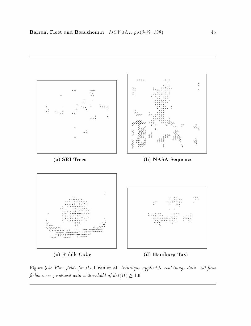
Barron, Fleet and Beauchemin IJCV 12:1, pp43-77, 1994 45

(a) SRI Trees (b) NASA Sequence(c) Rubik Cube (d) Hamburg TaxiFigure 5.4: Flow �elds for the Uras et al. technique applied to real image data. All ow�elds were produced with a threshold of det(H) � 1:0

Barron, Fleet and Beauchemin IJCV 12:1, pp43-77, 1994 46

(a) SRI Trees (b) NASA Sequence(c) Rubik Cube (d) Hamburg TaxiFigure 5.5: Flow �elds for the technique of Anandan applied to real image data. Theresults are unthresholded.

Barron, Fleet and Beauchemin IJCV 12:1, pp43-77, 1994 47

(a) SRI Trees (b) NASA Sequence(c) Rubik Cube (d) Hamburg TaxiFigure 5.6: Flow �elds produced by the technique of Singh applied to real image data. All ow �elds are computed with n = 2, w = 2 and N = 4. No thresholding was employed.

Barron, Fleet and Beauchemin IJCV 12:1, pp43-77, 1994 48(a) SRI Trees (b) NASA Sequence(c) Rubik Cube (d) Hamburg TaxiFigure 5.7: Flow �elds for the technique of Heeger applied to real image data. The resultsshown for Heeger's method were based on all 3 levels of the Gaussian pyramid, choosingthe estimates with speeds that are consistent from their respective levels of the pyramid (asdiscussed in Section 2.1). When consistent estimates are produced from more than onelevel, we choose the velocity estimate from the lowest level.

Barron, Fleet and Beauchemin IJCV 12:1, pp43-77, 1994 49

(a) SRI Trees (b) NASA Sequence(c) Rubik Cube (d) Hamburg TaxiFigure 5.8: Flow �elds for the technique of Waxman et al. applied to real image data.All ow �elds were produced with a spatial standard deviation of 1.5.

Barron, Fleet and Beauchemin IJCV 12:1, pp43-77, 1994 50

(a) SRI Trees (b) NASA Sequence(c) Rubik Cube (d) Hamburg TaxiFigure 5.9: Flow �elds for the Fleet and Jepson technique applied to real image data.All ow �elds were produced with a threshold of � = 1:25. Other parameters were identicalto those used by Fleet.

Barron, Fleet and Beauchemin IJCV 12:1, pp43-77, 1994 51Both real and synthetic image sequences were used to test the techniques. In bothcases, we chose sequences that are not severely corrupted by spatial or temporal aliasing.Of these di�erent techniques on the sequences we tested, we �nd that the most re-liable were the �rst-order, local di�erential method of Lucas and Kanade, and the localphase-based method of Fleet and Jepson. Although not as consistent, the second-orderdi�erential method of Uras et al. also performed well. Only these approaches performedconsistently well over all of the image sequences tested, with measures of con�dence atthe di�erent stages of computation to detect and/or remove unreliable measurements.The lack of reliable con�dence measures is a serious limitation of several of the otherapproaches.With respect to the class of di�erential approaches tested we can draw several conclu-sions of general interest. The �rst concerns the importance of numerical di�erentiationand spatiotemporal smoothing. With both �rst and second-order di�erential techniques,the method of numerical di�erentiation is very important { di�erences between �rst-orderpixel di�erencing and higher-order central-di�erences were very noticeable. Along thesame lines, some degree of spatiotemporal presmoothing to remove small amounts of tem-poral aliasing and improve the subsequent derivative estimates had a marked e�ect onthe quantitative accuracy of the resulting velocity estimates. The temporal smoothingwas particularly useful. These factors are perhaps most evident in comparing the resultsobtained with Horn and Schunck's original algorithm with those of our modi�ed versionof it. For the data tested we found a spatio-temporal standard deviation of � = 1:5 to benearly optimal.Another �nding concerns the methods used to combine local di�erential constraintsto obtain the 2-d velocity estimates. We found that the local explicit methods (i.e. local�ts to constant or linear models of v) were superior in both accuracy and computationale�ciency to global smoothness constraints (with energy functionals that penalize a lackof smoothness), used by Horn and Schunck [32] and Nagel [43]. We also found the lo-cal methods to be more robust with respect to errors in gradient measurement causedby quantization noise. A clear example of the di�erence between the two approaches isapparent in the di�erent errors produced the Lucas and Kanade method with those ofour modi�ed version of the Horn and Schunck method, since they share the same spa-tiotemporal derivative estimates. One of the main reasons for this distinction concernsthe existence of a con�dence measure to distinguish estimates of normal velocity from 2-dvelocity. In the case of Lucas and Kanade's method, we found that the size of the smallesteigenvalue of the normal equations in (2.9) was one such reliable measure. By contrast,

Barron, Fleet and Beauchemin IJCV 12:1, pp43-77, 1994 52we did not �nd a similarly good con�dence measure for Horn and Schunck's method.Finally we found that, contrary to much of the literature, second-order di�erentialmethods (e.g. [56, 57]) are capable of producing accurate and relatively dense measure-ments of 2-d velocity. Moreover, the determinant of the (spatial) Hessian I(x; t) was areasonably good con�dence measure, and signi�cantly more e�ective than its conditionnumber (suggested by Uras et al. [57]). One problem with this technique however, appearsto be its consistency. While it produced good results with predominantly translationalimage sequences, it appears to degrade faster than �rst-order techniques as the amount ofhigher-order geometric deformation in the input (e.g. dilation) increases. This is evidentwhen comparing the results from the Translating Tree and Diverging Tree sequences.As discussed above, this problem is consistent with the underlying assumptions of theapproach.We now turn to the matching techniques, both of which produced results that weregenerally poorer than those from the better di�erential methods. One of the main prob-lems we �nd with the SSD-based matching techniques is their ability to estimate sub-pixeldisplacements. With image translation and higher speeds they appear to perform well,but when the motion �eld involves small velocities with a signi�cant dilational compo-nent the estimated displacements are often poor. In these cases it appears that SSD-basedestimates of displacements are more accurate with integer displacements than subpixelvelocities.As a result of the relatively poor displacement estimates from the SSD minimization,the neighbourhood smoothness constraints employed by both Singh and Anandan areimportant to the success of these methods. At the same time, however, we found thatthe con�dence measures suggested for both approaches were not very e�ective. Thecon�dence measures suggested by Singh appeared to work somewhat better than thoseof Anandan's technique, in that they were generally correlated with the velocity errors.A problem in Anandan's approach, like that of Horn and Schunck was the inability todistinguish normal from 2-d estimates. In Singh's technique, they were more e�ective forstep 1 of the computation than for the �nal velocity estimates of step 2, where they werelargely ine�ective. While matching techniques did not produce the most accurate velocityestimates among the techniques we examined, it should be restated that, as compared tothe relatively large temporal duration of support used by the most successful techniques,these matching approaches used either 2 or 3 frames only.The �nal techniques considered include energy-based techniques and phase-based ap-proaches. Although there exist a number of interesting energy-based approaches, we have

Barron, Fleet and Beauchemin IJCV 12:1, pp43-77, 1994 53tested just one in this paper, namely the approach of Heeger [30]. Our results suggest thatthis technique is not as reliable as several of the other techniques considered. Althoughnot reported in detail here we found that the original nonlinear optimization suggested byHeeger to solve (2.28) was extremely sensitive to initial conditions and did not producereliable results. Our implementation of a parallel search method was better, but still leftmuch to be desired; of course, in part this may be due to our implementation. It appearshowever that the e�ort needed to solve the optimization problem, combined with the as-sumptions underlying the approach (e.g. translating white noise) will make this approachdi�cult to employ.The phase-based approach of Fleet and Jepson [23, 20] produced the most accurateresults overall. However, there are several issues worth noting for our implementation ofthis technique. First, we �nd that this technique is sensitive to temporal aliasing in theimage sequences because of the frequency tuning of the �lters. A second issue concerns thepotential number of con�dence measures. Fleet and Jepson proposed several constraintson phase stability and signal contrast (SNR) to weed out poor normal velocity estimates.It would be useful to have these combined into a single con�dence measure that wouldfacilitate a more general weighted LS solution to the 2-d velocities. A third problemwith our current implementation of the phase-based is its high computational load. LikeHeeger's method and other frequency-based methods, it involves a large number of �lters,which at present is the main computational expense. However, we expect that with theappropriate hardware in the near future the �ltering should cease to be a severe limitation,and all these techniques could be implemented at frame-rates. It is also important to notethat all our �lter outputs were stored in oating point and were not subsampled (exceptin cases involving the Laplacian pyramid). More e�cient encodings of the �lter outputshould be possible with subsampling and quantization of the �lter outputs as in [20] withonly slight reductions in accuracy.Finally, it is important to restate and qualify the conditions under which these testswere performed. First, we assumed that temporal aliasing was not a severe problem andthat intensity (or �ltered versions) were di�erentiable. As discussed earlier, if temporalaliasing is severe, then other approaches must be considered, such as coarse-to-�ne controlstrategies. Second, we have considered relatively simple image sequences, without largeamounts of occlusion, specularities, multiple motions, etc. and our quantitative measuresof performance should be taken as lower bounds on the expected accuracy under moregeneral conditions. Third, most of the implementations considered here involved onlyone scale of �ltering, and would produce better results with multi-scale implementations.

Barron, Fleet and Beauchemin IJCV 12:1, pp43-77, 1994 54This is true of most techniques, including those of Lucas and Kanade [40, 41] and thephase-based approach of Fleet and Jepson [20, 23].Acknowledgements: We thank the authors of the techniques examined here whoshared their insights and helped get the programs running. This work has been supportedin part by NSERC Canada, the Government of Ontario (through ITRC centres) and theGovernment of Canada (through IRIS).References[1] Adelson E.H. and Bergen J.R. (1985) Spatiotemporal energy models for the percep-tion of motion. J. Opt. Soc. Am. A2, pp. 284-299[2] Adelson E.H. and Bergen J.R. (1986) The extraction of spatiotemporal energy inhuman and machine vision. Proc. IEEE Workshop on Visual Motion, Charleston,pp. 151-156[3] Aloimonos J. and Brown C.M. (1984) Direct processing of curvilinear sensor mo-tion from a sequence of perspective images. Proc. Workshop on Computer Vision,Annapolis, pp. 72-77[4] Aloimonos Y. and Z. Duric (1992) Active egomotion estimation: a qualitative ap-proach. Proc. ECCV, Ligure, Italy, pp. 497-510[5] Anandan P. (1987) Measuring Visual Motion from Image Sequences. PhD disserta-tion, COINS TR 87-21, Univ. of Massachusetts, Amherest, MA[6] Anandan P. (1989) A computational framework and an algorithm for the measure-ment of visual motion. Int. J. Comp. Vision 2, pp. 283-310[7] Barman H., Haglund L. Knutsson H. and Granlund G. (1991) Estimation of veloc-ity, acceleration and disparity in time sequences. Proc. IEEE Workshop on VisualWorkshop, Princeton, pp. 44-51[8] Barron, J.L., Fleet, D.J., Beauchemin, S.S., and Burkitt, T. (1992) Performance ofoptical ow techniques. IEEE Conf. CVPR, Champaign, June, pp. 236-242[9] Barron J.L., Fleet D.J., and Beauchemin S.S. (1992) Performance of optical ow tech-niques. Technical Report: TR299, Dept. of Computer Science, University of Western

Barron, Fleet and Beauchemin IJCV 12:1, pp43-77, 1994 55Ontario; and RPL-TR-9107, Dept. of Computing Science, Queens University, July1992 (revised July 1993).[10] Barron J.L. Jepson A.D. and Tsotsos J.K. (1990) The feasibility of motion andstructure from noisy time-varying image velocity information. Int. J. Comp. Vision5, pp. 239-269[11] Bigun J,. Granlund, G. and Wiklund J. (1991) Multidimensional orientation estima-tion with applications to texture analysis and optical ow. IEEE Trans. PAMI, 13,pp. 775-790[12] Beaudet P.R. (1978) Rotationally invariant image operators. Proc. ICPR, pp. 579-583[13] Burt P.J. and Adelson E.H. (1983) The Laplacian pyramid as a compact image code.IEEE Trans. on Communications 31, pp. 532-540[14] Burt P.J., Yen C. and Xu X. (1983) Multiresolution ow-through motion analysis.Proc. IEEE CVPR, Washington, pp. 246-252[15] Buxton B. and Buxton H. (1984) Computation of optic ow from the motion of edgefeatures in image sequences. Image and Vision Computing 2, pp. 59-74[16] Cippola R. and Blake A. (1992) Surface orientation and time to contact from imagedivergence and deformation. Proc. ECCV Ligure, Italy, pp. 187-202[17] Duncan J.H. and Chou T.C. (1988) Temporal edges: The detection of motion andthe computation of optical ow. Proc. IEEE ICCV, Tampa, pp. 374-382[18] Dutta, R., Manmatha, R., Williams, L., and Riseman, E.M. (1989) A data set forquantitative motion analysis. Proc. IEEE CVPR, San Diego, pp. 159-164[19] Fennema C. and Thompson W. (1979) Velocity determination in scenes containingseveral moving objects. CGIP 9, pp. 301-315[20] Fleet D.J. and Jepson A.D. (1990) Computation of component image velocity fromlocal phase information. Int. J. Comp. Vision 5, pp. 77-104[21] Fleet D.J. and Jepson A.D. (1993) Stability of phase information. IEEE Trans. PAMI(in press)

Barron, Fleet and Beauchemin IJCV 12:1, pp43-77, 1994 56[22] Fleet D.J. and Langley K. (1993) Toward real-time optical ow. Proc. Vision Inter-face, Toronto, pp. 116-124 (also see Technical Report: RPL-TR-9308, Robotics andPerception Laboratory, Queen's University)[23] Fleet D.J. (1992) Measurement of Image Velocity. Kluwer Academic Publishers, Nor-well[24] Girosi F., Verri A. and Torre V. (1989) Constraints for the computation of optical ow. Proc. IEEE Workshop on Visual Motion, Irvine, pp. 116-124[25] Glazer F., Reynolds G. and Anandan P. (1983) Scene matching through hierarchicalcorrelation. Proc. IEEE CVPR, Washington, pp. 432-441.[26] Grzywacz N.M. and Yuille A.L. (1990) A model for the estimation of local imagevelocity by cells in the visual cortex. Proc. Roy. Soc. London B239, pp. 129-161[27] Haglund L. (1992) Adaptive Multidimensional Filtering. PhD Dissertation, Dept.Electrical Engineering, Univ. of Linkoping (ISSN 0345-7524)[28] Hildreth E.C. (1984) The computation of the velocity �eld. Proc. Roy. Soc. LondonB221, pp. 189-220[29] Heeger D.J. (1987) Model for the extraction of image ow. J. Opt. Soc. Am. A4, pp.1455-1471[30] Heeger D.J. (1988) Optical ow using spatiotemporal �lters. Int. J. Comp. Vision 1,pp. 279-302[31] Horn B.K.P. (1986) Robot Vision. MIT Press, Cambridge[32] Horn B.K.P. and Schunck B.G. (1981) Determining optical ow. AI 17, pp. 185-204[33] Horn B.K.P. and Weldon Jr. E.J. (1988) Direct methods for recovering motion. Int.J. Comp. Vision, 2, pp. 51-76[34] Jahne B. (1987) Image sequence analysis of complex physical objects: nonlinear smallscale water surface waves. Proc. IEEE ICCV London, pp. 191-200[35] Jepson A.D. and Fleet D.J. (1991) Phase singularities in scale-space. Image andVision Computing 9, pp. 338-343

Barron, Fleet and Beauchemin IJCV 12:1, pp43-77, 1994 57[36] Jepson A.D. and Heeger D.J. (1990) Subspace Methods for Recovering Rigid Motion,Part II: Theory, Int. J. Comp. Vision, (to appear)[37] Kearney J.K., Thompson W.B. and Boley D.L. (1987) Optical ow estimation: Anerror analysis of gradient-based methods with local optimization. IEEE Trans. onPAMI 9, pp. 229-244[38] Little J.J., Bultho� H.H. and Poggio T.A. (1988) Parallel optical ow using localvoting. Proc. IEEE ICCV, Tampa, pp. 454-459[39] Little J.J. and Verri A. (1989) Analysis of di�erential and matching methods foroptical ow. IEEE Workshop on Visual Motion, Irvine CA, pp. 173-180[40] Lucas B.D. (1984) Generalized Image Matching by the Method of Di�erences. PhDDissertation, Dept. of Computer Science, Carnegie-Mellon University[41] Lucas, B. and Kanade, T. (1981) An iterative image registration technique with anapplication to stereo vision. Proc. DARPA IU Workshop, pp. 121-130[42] Marr D. and Hildreth E.C. (1980) Theory of edge detection. Proc. Roy. Soc. London,B207, 1980, pp. 187-217[43] Nagel H.H. (1983) Displacement vectors derived from second-order intensity varia-tions in image sequences. CGIP 21, pp. 85-117[44] Nagel H.-H. (1987) On the estimation of optical ow: Relations between di�erentapproaches and some new results. AI 33, pp. 299-324[45] Nagel H.-H. (1989) On a constraint equation for the estimation of displacement ratesin image sequences. IEEE Trans. PAMI 11, pp. 13-30[46] Nagel H.H. and Enkelmann W. (1986) An investigation of smoothness constraintsfor the estimation of displacement vector �elds from image sequences. IEEE Trans.PAMI 8, pp. 565-593[47] Negahdaripour S. and Horn B.K.P. (1987) Direct passive navigation. IEEE Trans.PAMI 9, pp. 168-176[48] Tistarelli M. and Sandini G. (1990) Estimation of depth from motion using anthro-pomorphic visual sensor. Image and Vision Computing, 8, pp. 271-278

Barron, Fleet and Beauchemin IJCV 12:1, pp43-77, 1994 58[49] Santen J.P.H. van and Sperling G. (1985) Elaborated Reichardt detectors. J. Opt.Soc. Am. A2, pp. 300-321[50] Schunck B.G. (1984) The motion constraint equation for optical ow. Proc. ICPRMontreal, pp. 20-22[51] Schunck B.G. (1986) Image ow continuity equations for motion and density. Proc.IEEE Workshop on Visual Motion, Charleston, pp. 89-94[52] Simoncelli E.P., Adelson E.H. and Heeger D.J. (1991) Probability distributions ofoptical ow. IEEE Proc. of CVPR, Maui pp. 310-315[53] Simoncelli E.P. (1993) Distributed Representation and Analysis of Visual Motion.PhD Dissertation, Dept. of Electrical Engineering and Computer Science, MIT[54] Singh A. (1990) An estimation-theoretic framework for image- ow computation.Proc. IEEE ICCV, Osaka, pp. 168-177[55] Singh A. (1992) Optic Flow Computation: A Uni�ed Perspective. IEEE ComputerSociety Press,[56] Tretiak O. and Pastor L. (1984) Velocity estimation from image sequences with sec-ond order di�erential operators. Proc. IEEE ICPR, Montreal, pp. 20-22[57] Uras S., Girosi F., Verri A. and Torre V. (1988) A computational approach to motionperception. Biol. Cybern. 60, pp. 79-97[58] Verri A. and Poggio T. (1987) Against quantitative optical ow. Proc. IEEE ICCV,London, pp. 171-180[59] Watson A.B. and Ahumada A.J. (1985) Model of human visual-motion sensing. J.Opt. Soc. Am. A2, pp. 322-342[60] Waxman A.M. and Wohn K. (1985) Contour evolution, neighbourhood deformationand global image ow: Planar surfaces in motion. Int. J. Rob. Res. 4, pp. 95-108[61] Waxman A.M., Wu J. and Bergholm F. (1988) Convected activation pro�les andreceptive �elds for real time measurement of short range visual motion. Proc. IEEECVPR, Ann Arbor, pp. 717-723[62] Willick D. and Yang Y.H. (1991) Experimental evaluation of motion constraintsequations. CVGIP: Image Understanding, 54, pp. 206-214

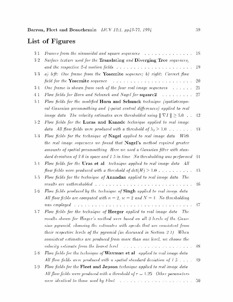
Barron, Fleet and Beauchemin IJCV 12:1, pp43-77, 1994 59List of Figures3.1 Frames from the sinusoidal and square sequences. : : : : : : : : : : : : : : 183.2 Surface texture used for the Translating and Diverging Tree sequences,and the respective 2-d motion �elds. : : : : : : : : : : : : : : : : : : : : : : 193.3 a) left: One frame from the Yosemite sequence; b) right: Correct ow�eld for the Yosemite sequence. : : : : : : : : : : : : : : : : : : : : : : : 203.4 One frame is shown from each of the four real image sequences. : : : : : : 214.1 Flow �elds for Horn and Schunck and Nagel for square2. : : : : : : : : : 275.1 Flow �elds for the modi�ed Horn and Schunck technique (spatiotempo-ral Gaussian presmoothing and 4-point central di�erences) applied to realimage data. The velocity estimates were thresholded using k rI k � 5:0. : : 425.2 Flow �elds for the Lucas and Kanade technique applied to real imagedata. All ow �elds were produced with a threshold of �2 � 1:0 : : : : : : : 435.3 Flow �elds for the technique of Nagel applied to real image data. Withthe real image sequences we found that Nagel's method required greateramounts of spatial presmoothing. Here we used a Gaussian �lter with stan-dard deviation of 3.0 in space and 1.5 in time. No thresholding was performed. 445.4 Flow �elds for the Uras et al. technique applied to real image data. All ow �elds were produced with a threshold of det(H) � 1:0 : : : : : : : : : : 455.5 Flow �elds for the technique of Anandan applied to real image data. Theresults are unthresholded. : : : : : : : : : : : : : : : : : : : : : : : : : : : : 465.6 Flow �elds produced by the technique of Singh applied to real image data.All ow �elds are computed with n = 2, w = 2 and N = 4. No thresholdingwas employed. : : : : : : : : : : : : : : : : : : : : : : : : : : : : : : : : : : 475.7 Flow �elds for the technique of Heeger applied to real image data. Theresults shown for Heeger's method were based on all 3 levels of the Gaus-sian pyramid, choosing the estimates with speeds that are consistent fromtheir respective levels of the pyramid (as discussed in Section 2.1). Whenconsistent estimates are produced from more than one level, we choose thevelocity estimate from the lowest level. : : : : : : : : : : : : : : : : : : : : 485.8 Flow �elds for the technique ofWaxman et al. applied to real image data.All ow �elds were produced with a spatial standard deviation of 1.5. : : : : 495.9 Flow �elds for the Fleet and Jepson technique applied to real image data.All ow �elds were produced with a threshold of � = 1:25. Other parameterswere identical to those used by Fleet. : : : : : : : : : : : : : : : : : : : : : 50

Barron, Fleet and Beauchemin IJCV 12:1, pp43-77, 1994 60List of Tables4.1 Summary of Sinusoid 1 Results. See the text for a discussion of theseresults and the apparent anomalies. : : : : : : : : : : : : : : : : : : : : : : 254.2 Summary of Square2 2D Velocity Results. : : : : : : : : : : : : : : : : : : 284.3 Summary of Square2 Normal/Component Velocity Results. : : : : : : : : 294.4 Summary of the Translating Tree 2D Velocity Results. : : : : : : : : : : 324.5 Summary of the Diverging Tree 2D Velocity Results. : : : : : : : : : : : 334.6 Summary of Diverging Tree Normal/Component Velocity Results. : : : : 354.7 Summary of Yosemite 2D Velocity Results : : : : : : : : : : : : : : : : : 36