CS229T/STATS231: Statistical Learning Theory

Lecturer: Tengyu Ma Lecture 11Scribe: Jongho Kim, Jamie Kang October 29th, 2018

1 Overview

This lecture mainly covers

• Recall the statistical theory of GANs from the last lecture

• Introduce Kontorovich-Rubinstein duality of Wasserstein distance and provide theproof

2 Review

Recall the following notations and two definitions from the last lecture:

z1, . . . , zni.i.d∼ Z where Z ∼ N (0, Ik×k)

X = Gθ(Z) : Gθ is the generator Rk → Rd

x1, . . . , xni.i.d∼ P : training examples

p̂ : Uniform distribution over {x1, . . . , xn}

pθ : distribution of X = Gθ(Z)

p̂θ : uniform distribution over {Gθ(z1), . . . , Gθ(zm)}

Definition 1 (Wasserstein Distance).

W1(P,Q) = sup‖f‖L≤1

Ex∼P [f(x)]− Ex∼Q [f(x)]

Here, the supremum is over functions f where f is 1-Lipschitz continuous function withrespect to metric d. For simplicity, we denote this as ‖f‖L ≤ 1. Recall that the function fis 1-Lipschitz continuous if

|f(x)− f(y)| ≤ d(x, y) ∀x, y

Most of cases, we let the metric d to be l2 distance.

Definition 2 (F-Integral Probability Metric (F-IPM)).

WF (P,Q) = supf∈F

|Ex∼P [f(x)]− Ex∼Q [f(x)]|

where F is a family of functions (e.g., a family of neural nets {fφ}).

This week (week 6), we would like to address the following question:

WF (p̂, p̂θ)︸ ︷︷ ︸training loss

small =⇒ W1 (p, pθ) small ?

3 Duality of W1 (Kontorovich-Rubinstein duality)

Theorem 1. Let P , Q be two distributions over X (assume P and Q have boundedsupport) and let d be a metric on X . Then, we have

W1(P,Q) = sup‖f‖L≤1

Ex∼P [f(x)]− Ex∼Q [f(x)]

= infP

E(x,y)∼P [d(x, y)] (1)

where P is coupling of P and Q. A coupling P is a joint distribution over X × X whosemarginals are P and Q. (i.e., If (x, y) ∼ P then Px = P and Py = Q.)

Equivalently, we can think of coupling as if we are sending mass from X to X . Suppose wehave a finite set X such that X = {v1, . . . , vk}. Let P and Q be the two distributions overX as following:

P = (p1, . . . , pk) where∑

i pi = 1 and pi ≥ 0 ∀i

Q = (q1, . . . , qk) where∑

i qi = 1 and qi ≥ 0 ∀i

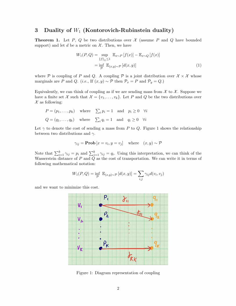
Let γ to denote the cost of sending a mass from P to Q. Figure 1 shows the relationshipbetween two distributions and γ.

γij = Prob [x = vi, y = vj ] where (x, y) ∼ P

Note that∑k

i=1 γij = pi and∑k

j=1 γij = qi. Using this interpretation, we can think of theWasserstein distance of P and Q as the cost of transportation. We can write it in terms offollowing mathematical notation:

W1(P,Q) = infP

E(x,y)∼P [d(x, y)] =∑i,j

γijd(vi, vj)

and we want to minimize this cost.

Figure 1: Diagram representation of coupling

2

Last lecture, we shortly discussed why other distance measures (e.g., Total Variation (TV)distance and Kullback-Leibler(KL) divergence) are not useful in our setting compared toWasserstein distance. Before we move on to the formal proof of Theorem 1, here we discussand compare Wasserstein distance with TV distance and KL divergence.

Definition 3 (Total Variation distance).

TV(P,Q) = sup0≤f≤1

|Ex∼P [f(x)]− Ex∼Q [f(x)]| (All cases)

=1

2

∫|p(x)− q(x)| dx where P and Q have densities p and q (Continuous case)

Definition 4 (Kullback-Leibler divergence).

KL(P,Q) = Ex∼P[log

p(x)

q(x)

]=∑x

P (x) logP (x)

Q(x)(Discrete case)

=

∫ ∞−∞

p(x) log

(p(x)

q(x)

)dx (Continuous case)

Example 1. Suppose P is uniform distribution over sphere and Q is also uniform distri-bution over sphere which is shifted by ε on only one coordinate. Let the metric d = l2.Figure 2 shows two distributions of P and Q.

Figure 2: Distributions of P and Q

In this case, TV(P,Q) = 1 because we can construct the function f as following:

f(x) = 1 if X ∈ support(P )

f(x) = 0 if X ∈ support(Q)

Note that KL(P,Q) is not well-defined in this setting because not both P and Q defined onthe same probability space. On the other hand, W1(P,Q) ≤ ε. To see why this is the case,we first construct a coupling as following sampling technique:

(x, y) ∼ P ⇐⇒ x ∼ P, y = x+ ε

[10

]

3

Note that the marginal distribution would be P and Q. Here, we achieve

W1(P,Q) = E(x,y)∼P [d(x, y)]

= E(x,y)∼P [‖x− y‖2]

= ε since x− y = ε ·[10

]Example 2. We state the following claim:

Claim 1. TV(P,Q) = W1(P,Q) with respect to the trivial metric d(x, y) = I {x 6= y}(Note: This claim explains why TV distance does not take into account geometry.)

Proof. f is 1-Lipschitz with respect to the metric d(x, y) = I {x 6= y}. We claim that

|f(x)− f(y)| ≤ I {x 6= y} ⇐⇒ supx∈X

f(x)− inf(f) ≤ 1

To see this, first note that from |f(x)− f(y)| ≤ I{x 6= y}, we get that |f(x)− f(y)| ≤ 1 ifx 6= y. Thus, if the elements obtaining the sup and inf are not the same, then the differenceis bounded by 1, otherwise the difference will be 0. Furthermore, if supx∈X f(x)−inf(f) ≤ 1,it immediately follows that |f(x)− f(y)| ≤ 1 ∀x, y. This establishes the equivalence.

From here, we denote Ex∼P [f(x)] = Ex∼P f and Ex∼Q [f(x)] = Ex∼Qf for simplicity.Then,

W1(P,Q) = supf :sup f−inf f≤1

Ex∼P f − Ex∼Qf︸ ︷︷ ︸shift invariant

= supf :0≤f≤1

Ex∼P f − Ex∼Qf

= maxf :0≤f≤1,0≤1−f≤1

{Ex∼P f − Ex∼Qf, Ex∼P (1− f)− Ex∼Q(1− f)}

= sup0≤f≤1

|Ex∼P f − Ex∼Qf |

= TV (P,Q)

where the second equality follows from the fact that Ex∼P f −Ex∼Qf is shift invariant (i.e.,EP [f + c]−EQ[f + c] = EP f + c−EQf − c = EP f −EQf), and thus we can subtract inf f .The fourth equality is again using the fact that Ex∼P (1−f)−Ex∼Q(1−f) is shift invariantand thus we can remove 1 and have the second term become EP (−f)− EQ(−f).

3.1 Proof of Kontorovich-Rubinstein duality

We use LP duality in fuctional space with f as variable to prove Theorem 1.

Assume X is finite: X = {v1, ..., vk} and f(v1), ..., f(vk) , (f1, ..., fk) and recall thatP = (p1, ..., pk), Q = (q1, ..., qk). As usual, we assume pi > 0, qi > 0 for all i. We con-struct the following linear programming problems:

4

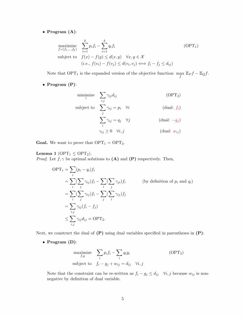
• Program (A):

maximizef=(f1,...,fk)

k∑i=1

pifi −k∑i=1

qifi (OPT1)

subject to f(x)− f(y) ≤ d(x, y) ∀x, y ∈ X(i.e., f(vi)− f(vj) ≤ d(vi, vj)⇐⇒ fi − fj ≤ dij)

Note that OPT1 is the expanded version of the objective function: maxf

EP f − EQf .

• Program (P):

minimizeγ

∑i,j

γijdij (OPT2)

subject to∑j

γij = pi ∀i (dual: fi)∑i

γij = qj ∀j (dual: −gj)

γij ≥ 0 ∀i, j (dual: wij)

Goal. We want to prove that OPT1 = OPT2.

Lemma 1 (OPT1 ≤ OPT2).Proof. Let f, γ be optimal solutions to (A) and (P) respectively. Then,

OPT1 =∑i

(pi − qi)fi

=∑i

(∑j

γij)fi −∑i

(∑j

γji)fi (by definition of pi and qi)

=∑i

(∑j

γij)fi −∑j

(∑i

γij)fj

=∑i,j

γij(fi − fj)

≤∑i,j

γijdij = OPT2.

Next, we construct the dual of (P) using dual variables specified in parentheses in (P):

• Program (D):

maximizef,g

∑i

pifi −∑i

qigi (OPT3)

subject to fi − gj + wij = dij ∀i, j

Note that the constraint can be re-written as fi − gj ≤ dij ∀i, j because wij is non-negative by definition of dual variable.

5

Lemma 2 (OPT1 ≥ OPT3).Proof. The main idea here is to use the fact that d is a metric. Let f, g, γ be optimalsolutions to (P) and (D). Then, by complementary slackness1,

fi − gj = dij if γij > 0 ∀i, j.

First, we show that gj − gt ≤ djt ∀j, t by following

∀j, pick i such that γij > 0 =⇒ fi − gj = dij (1)

Also, by constraint: ∀i, t fi − gt ≤ dit (2)

(1)− (2) yields: gj− gt ≤ dit−dij ≤ djt where the last inequality is from triangle inequalityas d is a metric. Therefore, g is a feasible solution of (A). Note that from (D)’s constraint,fi − gi ≤ dii and dii = 0 since it’s a metric. Therefore, fi ≤ gi for all i. Using this, weobtain:

OPT1 ≥∑i

pigi −∑i

qigi (feasibility of g)

≥∑i

pifi −∑i

qigi (fi ≤ gi)

= OPT3.

Finally, by Lemma 1 and Lemma 2 and the fact that OPT2 = OPT32, we conclude

OPT1 = OPT2 = OPT3.

4 Plans for future lectures

Recall that the main question we aim to address is:

WF (p̂, p̂θ)︸ ︷︷ ︸training loss

small =⇒ W1 (p, pθ) small ?

Our plan for addressing this question is following:

Plan: WF (p̂, p̂θ)generalization←−−−−−−−→ WF (p, pθ)

approx.W1≈WF←−−−−−−−−→ W1(p, pθ).

Hence, in the next lecture we will show three observations:

1. If F is complex =⇒ generalization is bad

2. If F has small complexity =⇒ generalization is good

3. If F has small complexity =⇒ approximation may not be good

and explore ways to overcome this dilemma.

1If you are not familiar with this part, please refer to Chapter 5 of Convex Optimization [?] and/or EE364A course lecture slide 17 on http://web.stanford.edu/class/ee364a/lectures/duality.pdf

2Since OPT3 is dual of OPT2 and strong duality holds for linear programming, OPT2 = OPT3.

6