1

Outlier Detection for Robust Multi-dimensionalScaling

Leonid Blouvshtein, Daniel Cohen-Or

Abstract—Multi-dimensional scaling (MDS) plays a central role in data-exploration, dimensionality reduction and visualization.State-of-the-art MDS algorithms are not robust to outliers, yielding significant errors in the embedding even when only a handful ofoutliers are present. In this paper, we introduce a technique to detect and filter outliers based on geometric reasoning. We test thevalidity of triangles formed by three points, and mark a triangle as broken if its triangle inequality does not hold. The premise of ourwork is that unlike inliers, outlier distances tend to break many triangles. Our method is tested and its performance is evaluated onvarious datasets and distributions of outliers. We demonstrate that for a reasonable amount of outliers, e.g., under 20%, our method iseffective, and leads to a high embedding quality.

F

1 INTRODUCTION

MUlti-dimensional Scaling (MDS) is a fundamentalproblem in data analysis and information visualiza-

tion. MDS takes as input a distance matrix D, containingall(N2

)pairs of distances between elements xi, and embeds

the elements in d dimensional space such that the pairwisedistancesDij are preserved as much as possible by ||xi−xj ||in the embedded space. When the distance data is outlier-free, state-of-the-art methods (e.g., SMACOF) provide sat-isfactory solutions [1], [2]. These solutions are based on anoptimization of the so-called stress function, which is a sumof squared errors between the dissimilarities Dij and theircorresponding embedding inter-vector distances:

StressD(x1, x2, ...xN ) =∑i6=j

(Dij − ||xi − xj ||)2.

In many real-world scenarios, input distances may benoisy or contain outliers, due to malicious acts, systemfaults, or erroneous measures. Many MDS techniques dealwith noisy data [3], [4], but little attention has been givento outliers [5], [6], [7]. We refer to outliers as opposed tonoise, as distances that are significantly different than theircorresponding true values.

Developing a robust MDS is challenging since even asmall portion of outliers can lead to significant errors. Thissensitivity of MDS to outliers is demonstrated in Figure 1,where only two pairwise distances (out of 435 pairs) areerroneous (colored in red in (a)), cause a strong distortion inthe embedding (b). To highlight the embedding errors, wedraw lines connecting between the ground truth positionsand the embedded positions.

In this paper, we introduce a robust MDS technique,which detects and removes outliers from the data and henceprovides a better embedding.

Our approach is based on geometric reasoning withwhich the outliers can be identified by analyzing the giveninput distances. This approach follows the well-known id-iom ”prevention is better than a cure”. That is, instead ofrecovering from the damage that the outliers cause to the

0 5 10 15 20 25-15

-10

-5

0

5

10

-20 -10 0 10 20 30 40-30

-20

-10

0

10

20

30

Fig. 1: Two outlier distances (marked in dashed lines onthe left) lead to a significant distortion in the embedding,as reflected by the large offsets between ground-truth andembedded positions, shown on the right.

MDS optimization, we prevent them in the first place, bydetecting and filtering them out.

We treat the distances as a complete graph of(N2

)edges.

Each edge is associated with its corresponding distance andforms N − 2 triangles with the rest of the N − 2 nodes.The premise of our work is that an outlier distance tends tobreak many triangles. We refer to a triangle as broken if itstriangle inequality does not hold. As we shall show, whileinlier edges participate in a rather small number of brokentriangles, outlier edges participate in many. This allows usto set a conservative threshold and classify the edges andtheir associated distances as inliers and outliers (See Figure2).

Generally speaking, MDS is an overdetermined problemsince the distance matrix contains many more distances thannecessary to solve the problem correctly. Hence, the ideais to detect distances that are suspected to be outliers andremove them before applying the MDS. In the following, wedenote and refer to our robust MDS method with TMDS.As we shall show, our technique succeeds in detectingand removing most of the outliers without any parameters,while incurring a rather small number of false positives, tofacilitate a more accurate embedding. We tested, analyzed

arX

iv:1

802.

0234

1v1

[cs

.CV

] 7

Feb

201

8

2

and evaluated our method on a large number of datasetswith varying portions of outliers from various distributions.

2 BACKGROUND

MDS was originally used and developed in the field of Psy-chology, as a means to visualize perceptual relations amongobjects [8], [9]. Nowadays, MDS is used in a wide variety offields, such as marketing [10], and graph embedding [11].Most notably, MDS plays a central role in data exploration[12], [13], [14], and computer graphics applications liketexture mapping [15], shape classification and retrieval [16],[17], [18] and more.

Several methods were suggested to handle outliers inthe data (e.g., [5], [7]). Using Sammon weighting [19] leadsto the following stress function:∑

i 6=j

(Dij − ||xi − xj ||)2

Dij.

This objective function can effectively be considered asrobust to elongated distances since it decreases the weightsof long distances. We differentiate between two types ofoutliers: larger and shorter outliers (colored in blue and red,respectively, in Figures 3 and 4), since their characteristicsand effects are different and may thus require differenttreatments. In (a) we show 2D data elements, where theoutliers are marked in red and blue. In (b) we show theirpositions recovered by applying a state-of-the-art MDS (i.e.,SMACOF) and in (c) the results of Sammon method [19].As can be observed, Sammon method can deal well withelongated distances, by assigning them with low weights.However, shortened distances are not dealt with well, asthey are assigned larger weights which lead to a distortedembedding.

The most related work to ours is the method presentedby Forero and Giannakis [6], hereafter referred to as FG12.They use an objective function F (X,O) that aims to find anembedding X and an outliers matrix O that minimize thefollowing:∑

i<j

(Dij − ||xi − xj || −Oij)2 + λ∑i<j

1(Oij 6= 0),

where λ regulates the number of non-zero values in O thatrepresent outliers.

Setting the size of λ to control the sparsity of Oij is noteasy. If λ is too big, too few outliers are detected; if it is toosmall, too many edges are treated as outliers. As we shallshow, close values of λ can lead to different results. Thisphenomenon is shown in Figure 5 (a-c). Thus, careful tuningof λ is required to achieve good results. This is an overlycomplex process, since, as well shall show, the algorithm isalso sensitive to the initial guess.

Note that X has d × N unknown variables and O has(N2

)variables. This amounts to a considerable increase in the

number of parameters, and hence it is significantly harderto optimize FG12 compared to SMACOF. This is evident inFigure 5 where we show (d-f) that with the same λ appliedto the same dataset, but with different initial guesses. Asshown, the three initial guesses yield a different numberof edges that are considered as outliers. This behavior of

the FG12 method can also be observed in Figure 6. Notethat for the yellow curve, λ = 1.8 is the value that detectsthe correct number of outliers. However, for the same valueof λ the blue plot detects most of the edges as outliers.This highlights the sensitivity of the FG12 method andemphasizes that we cannot set the value of λ even whenwe have a good estimation of the number of outliers in thesystem.

3 DETECTING OUTLIERS

Our technique estimates the likelihood of each distance to bean outlier. We treat the

(N2

)distances as a complete graph of(N

2

)edges connecting theN vertices. Each edge is associated

with its corresponding distance and forms N − 2 triangleswith the rest of the N − 2 elements. The key idea is thatinlier edges participate in a rather small number of brokentriangles, while outlier edges participate in many. As weshall see, by analyzing the histogram of broken triangles,we can set a conservative threshold and classify the edgesand their associated distances as inliers and outliers. SeeFigure 2.

Let D represent the pairwise distances among graphvertices. In the presence of outliers, some of the edges donot represent a correct Euclidean relation. In particular, anerroneous edge length tends to break a triangle formed bythe edge and its two endpoint vertices, and a third vertexfrom among the rest of the N −2 vertices. Recall that here, abroken triangle is one for which the triangle inequality doesnot apply.

We can easily identify all the broken triangles by travers-ing all triangles in the graph. For any triangle with edges oflength (d1, d2, d3) where d1 ≤ d2 ≤ d3, we test: d1 +d2 < d3We then count for each of the edges in the graph, thenumber of broken triangles it participates in. This yieldsa histogram H , where H(b) counts the number of edgesthat participate in b broken triangles. Figure 7 depicts sucha typical histogram. As can be observed, most of the edgesparticipate in a small number of broken triangles. The longtail of the histogram is associated with outliers.

It should be noted that an outlier edge does not neces-sarily break all its triangles, but in large numbers it standsout, and as we shall see, is likely to be detected.

We wish to determine a threshold φ to classify the outlier.That is, an edge which participates in more than φ brokentriangles is classified as an ourlier. The threshold φ cannotbe set to accurately classify the inlier/outlier edges. Instead,we propose a simple way to determine this threshold byanalyzing the histogramH . We set φ to be the smallest valuethat satisfies the following two requirements:

1)∑φb=1H(b) ≥ |E|/2

2) H(φ+ 1) > H(φ)

The first requirement assures that most of the edges arenot considered as outliers. This assumption holds in mostcases, but can be adjusted according to the problem setting.The second requirement corresponds to the observation thatoutlier edges tend to form a high bin along the tail of thehistogram H (Figure 7). This simple heuristic performs wellempirically (see Section 4).

3

-10 -8 -6 -4 -2 0 2 4 6 8 10-8

-6

-4

-2

0

2

4

6

8

10Factor:1. Broken Triangles 0

(a)

-10 -8 -6 -4 -2 0 2 4 6 8 10-8

-6

-4

-2

0

2

4

6

8

10Factor:0.77778. Broken Triangles 20

(b)

-10 -8 -6 -4 -2 0 2 4 6 8 10-8

-6

-4

-2

0

2

4

6

8

10Factor:0.33333. Broken Triangles 50

(c)

Fig. 2: The effect of distorting two distances, marked by red dashed lines (a). The green lines represent edges that violatethe triangle inequality (b). A stronger distortion leads to a larger number of broken triangles (c)

After the threshold is selected, we can remove the as-sociated distances from the data, and use the remainingdistances to compute an embedding using MDS. A high-level pseudo code of TMDS is described in Algorithm 1.

Algorithm 1: TMDS

Let D be a dissimilarity NxN matrix.;1. Calculate Countij - the number of broken triangleswhere the edge Dij participates.

2. Calculate the histogram H(b), where the bin H(b)counts the number of edges that participate inexactly b broken triangles.

3. Find the threshold φ according to 1 and 2.4. Let F be an N ×N matrix where:

Fij =

{0, Countij > φ

1, otherwise

}5. Execute a weighted MDS with an associated weightmatrix F .

4 ANALYSIS

4.1 Algorithm complexity

Testing all the triangles to identify the broken ones, amountsto a time complexity ofO(N3), an order of magnitude largerthan that of SMACOF (O(N2)). To avoid increasing the totaltime complexity of the MDS method, we can subsampleO(N2) triangles and build the histogram based only onthem. We can use uniform sampling, where, for every edge

-10 -8 -6 -4 -2 0 2 4 6 8 10-10

-8

-6

-4

-2

0

2

4

6

8

10

(a)

-20 -15 -10 -5 0 5 10 15 20-20

-15

-10

-5

0

5

10

15

20

25

(b)

-10 -8 -6 -4 -2 0 2 4 6 8 10-10

-8

-6

-4

-2

0

2

4

6

8

10

(c)

Fig. 3: (a) The blue lines represent the enlarged distances.(b) embedding with SMACOF. (c) Sammon embedding.

N SMACOF TMDS FG12150 2 4.84 15.9300 3.5 9.35 59.4450 5.5 19.6 105.5600 8.9 32.2 207.8750 13.5 46.9 309.4900 14.8 59.9 491.4

TABLE 1: CPU time in seconds of three embedding algo-rithms of data sampled uniformly from a 2d unit hypercubewith a various number (N ) of objects. The distance matrixwas contaminated with 10% outliers. All the methods wereimplemented in Matlab and tested on a single core of i3-6200U processor. For TMDS we sampled 100 triangles peredge, and for FG12 we used λ = 2. TMDS is faster thanFG12 and compared to SMACOF has a close to constantmultiplicative overhead, as expected.

Dij , we sample a constant number of points to form aconstant number of triangles. As can be observed in Figure8, testing too few triangles, may impair the detection rate.It can be seen that 45 triangles per edge are enough todetect most of the outliers, and that it scales well withN. Empirically, we observed that sampling twice as manytriangles as the expected number of outliers is an effectiverule-of-thumb. In practice, for N = 100 TMDS without anysub-sampling takes only 2 seconds using a non-optimizedimplementation in Matlab, while computing the embeddingitself using SMACOF takes 1.9 seconds. This suggests thatthe filtering step does not incur significant overhead. SeeTable 1.

-10 -8 -6 -4 -2 0 2 4 6 8 10-10

-8

-6

-4

-2

0

2

4

6

8

10

(a)

-10 -8 -6 -4 -2 0 2 4 6 8 10-10

-8

-6

-4

-2

0

2

4

6

8

10

(b)

-10 -8 -6 -4 -2 0 2 4 6 8 10-10

-8

-6

-4

-2

0

2

4

6

8

10

(c)

Fig. 4: (a) The blue lines represent the shortened distances.(b) embedding with SMACOF. (c) Sammon embedding.

4

-15 -10 -5 0 5 10 15-15

-10

-5

0

5

10

15Non-Zero(O) = 1118. λ = 0.1

(a)

-15 -10 -5 0 5 10 15-15

-10

-5

0

5

10

15Non-Zero(O) = 337. λ = 0.2

(b)

-15 -10 -5 0 5 10 15-15

-10

-5

0

5

10

15Non-Zero(O) = 101. λ = 0.3

(c)

-10 -8 -6 -4 -2 0 2 4 6 8 10-10

-8

-6

-4

-2

0

2

4

6

8

10λ = 1.5.

(d)

-15 -10 -5 0 5 10-10

-8

-6

-4

-2

0

2

4

6

8

10λ = 1.5.

(e)

-15 -10 -5 0 5 10 15-10

-5

0

5

10

15λ = 1.5.

(f)

Fig. 5: (a-c) Different λ applied to the same dataset with thesame initial guess, leads to different embedding qualities.(d-f) Same λ applied to the same datasets with differentinitial guesses, yields different embedding qualities.

4.2 Evaluation

To evaluate TMDS, we use synthesized data of various mag-nitudes, dimensions, and portions of outliers. We measurethe precision-recall performance of detecting the outliers,and the quality of the embedding with and without ouroutlier filtering. More precisely, we synthesize ground-truthdata by randomly sampling N points in a d dimensionalhypercube, and compute the pairwise distances D betweenthem. We randomly pick M elements and replace them witha random element from the distance matrix.

Qualitative evaluation. We use Shepard Diagrams to vi-sually display the classification of data elements as eitheroutliers or inliers. In the diagram in Figure 9, each point rep-resents a distance. The X-axis represents the input distancesand the Y-axis represents the distance in the embeddingresult. Points on the main diagonal are inliers representingthe distances that are correctly preserved in the embedding.The red circles represent the distances that TMDS detects asoutliers. The blue off-diagonal points are the false negatives,and the red dots on the diagonal are false positive distances.

0.4 0.6 0.8 1 1.2 1.4 1.6 1.8 2 2.2 2.4

λ

0

500

1000

1500

Non

Zer

o(O

)

N = 50

Fig. 6: This graph presents the number of non-zero elementsin O (which represent outliers) as a function of λ. Thethree plots were generated using different initial guessesthat were uniformly sampled. This suggests that the FG12method is overly sensitive to the initial guess. For thisexperiment we used N = 50 (1225 edges) and 100 outliers

1 2 3 4 5 6 7 8 9 10

Number of broken triangles

0

5

10

15

log

2(N

umbe

r O

f Edg

es) N = 40, Outliers = 20

Fig. 7: Histogram H(b) counts the number of edges thatbreak ’b’ triangles. It can be seen that most of the edgesbreak only a few triangles. The tail of the histogram isassociated with outliers. The y-axis is logarithmic to betterperceive the variance.

10 15 20 25 30 35 40 45

Triangles Sampled Per Edge

0.4

0.6

0.8

1

Out

liers

Det

ecte

d

N=50N=70N=90

Fig. 8: The number of outliers detected as a function of thenumber of subsampled per-edge triangles. The data consistsof 15 outliers.

The number of false positives and negatives increases as thenumber of outliers increases.

Quantitative evaluation. We employ two models to quan-titatively evaluate TMDS. In the first, we select outliers atrandom, while in the second all edges are distorted by alog-normal distribution.

First, we measure the accuracy of outlier detection usingprecision-recall. Each distance is classified as either inlier oroutlier, and the detection can thus be regarded as a retrievalprocess, where precision is the fraction of retrieved outliersthat are true positives, and recall is the fraction of truepositives that are detected. As can be observed in Figure 10,

0 50 100 150 200 250 300

Dnm

0

50

100

150

200

250

300

dnm

(X)

N = 100. Outliers = 2%

(a)

0 50 100 150 200 250 300

Dnm

0

50

100

150

200

250

300

dnm

(X)

N = 100. Outliers = 10%

(b)

Fig. 9: Shepard Diagram. Each point represents a distance.The X-axis represents the input distances and the Y-axisrepresents the distance in the embedding result. The redcircles represent the edges that are considered as outliers.(a) 2% outliers. (b) 10% outliers.

5

our precision and recall are high, where the first moderatelydecreases with the number of outliers and the latter in-creases. The precision is larger than 75%, which implies thata non-negligible portion of the filtered distances are falsepositives. However, the excess of filtering is not destructivesince MDS is an over-determined problem. Yet, at somepoint, filtering too many distances impairs the embedding,as will be demonstrated in a separate experiment below.

2 4 6 8 10 12 14 16 18 20

Number Of Outliers

0

0.5

1

N = 70

RecallPrecision

Fig. 10: Precision and Recall plot. N=70.

The detection probability. Figure 11 shows the probabil-ity of an outlier to be detected as a function of its errormagnitude, which is measured by the ratio between theactual distance dout and the true distance dGT . As can beobserved, edges that are strongly deformed (either squeezedor enlarged) are likely to be detected. This holds also forhigher dimensions.

-3 -2 -1 0 1 2 3

log2(Outlier Distance / GT Distance)

0

0.5

1

Det

ectio

n R

ate

N = 80. Outliers Rate = 5%

Dimension=2Dimension=3Dimension=4

Fig. 11: The outlier detection rate as a function of the shrink-age enlargement of the outliers relative to the ground-truthvalue. Edges that are strongly deformed (either squeezed orenlarged) are likely to be detected. Note that the X-axis islogarithmic: log2(dout/dGT ).

Embedding evaluation. To obtain insight about the em-bedding performance of points X1, ..., XN , we used thefollowing score:

Sij =

∣∣∣∣ log ||Xi −Xj ||Dij

∣∣∣∣Then, we take the average of Sij as the score for theembedding. This scoring treats shrinkage and enlargementsequally, where a low score implies a better embedding. Theresults of the evaluation are displayed in Figure 12. The plotshows that when the portion of outliers is less than 22%, ourpre-filtering performs better than applying SMACOF MDSdirectly. A larger amount of outliers causes TMDS to filterout too many inliers and impairs the embedding.Log-normal distribution. We generated synthetic data thatmimics realistic data characteristics, by sampling N data

points uniformly in a d-dimensional hypercube, and form-ing the respective distance matrix D. We distorted thedistances using factors of log-normal distribution. That is,every distance Dij is multiplied by a factor sampled froma log-normal distribution, where the log-normal mean is1. Note that these distorted distances include both noiseand outliers. The results of those simulations with differentlog standard deviation σ are presented in Figure 13. Notethat for larger σ values, which signify larger errors, theeffectiveness of TMDS is more significant.Non-uniform Distributions. We further evaluated TMDSon non-uniform structured data. The embedding of data setswith clear structures are shown in Figure 14. As we shalldiscuss below, one of the limitations of TMDS is handlingstraight lines. This is evident in Figure 14, where our em-bedding is imperfect (b), albeit better than without filtering(a). In (c-d), the structured data is numerically easier forfiltering. As demonstrated, the accuracy of the embeddingof the data with 15% outliers is high.

4.3 LimitationsAs described, our algorithm consists of two parts - buildingthe histogram of broken triangles and setting the thresh-old. Each part has it own limitations. The analysis of thehistogram assumes that outlier edges break many triangles,while inliers do not. This assumption may not hold when alarge number of triangles are broken also by inlier distances.This may happen when Dij = Dik + Dkj , but due tonumerical issues,Dij > Dik+Dkj , for example, when manypoints reside along straight lines. Setting the threshold φ ismerely a heuristic that may fail when there are too manyoutliers, or too few that have a special distribution thatconfuses the heuristics and causes half of the data to beconsidered as outliers.

5 EXPERIMENTS

A Matlab implementation is available at goo.gl/399buj.In the previous sections, we have tested and evaluated

our method (TMDS) using synthetic data for which wehave the ground truth distances. We have shown that theMDS technique of Forero and Giannakis [6] is sensitiveto the initial guess and its performance is dependent ona user-selected parameter. In the following, we evaluateour method on data for which the ground truth is notavailable. To evaluate the performance, we compare TMDS

0.05 0.1 0.15 0.2 0.25 0.3

Outliers Rate

0

0.1

0.2

0.3

Sco

re

N = 80

Filtered MDSSMACOF

Fig. 12: A comparison between SMACOF and TMDS asa function of outlier rate. Up to 22% TMDS has betterperformance.

6

0 0.2 0.4 0.6 0.8 1 1.2 1.4 1.6 1.8 2

σ

0

2

4

6

Sco

re

N = 50

Filtered MDSSMACOF

Fig. 13: A comparison between SMACOF and TMDS forvarious distributions defined as a function of σ.

0 5 10 15 20 25

-10

-5

0

5

10

SMACOF

0 5 10 15 20 25

-10

-5

0

5

10

TMDS

0 20 40 60 80 100 120-60

-40

-20

0

20

40

60

SMACOF

0 20 40 60 80 100 120-60

-40

-20

0

20

40

60

TMDS

Fig. 14: The embedding of a ’PLUS’ shaped dataset (upperrow) with 10% outliers, and a ’SPIRAL’ shaped dataset(bottom row) with 15% outliers. Each embedding point isconnected to its ground-truth point.

with a SMACOF implementation of MDS using numerouscommon measures that assume ground truth labels, but notdistances. The labels are used for evaluation only. First, wetest TMDS on two real datasets available on the Web, forwhich the ground truth distances are available. Next, weevaluate TMDS on three datasets for which ground truthdistances are unavailable, but classes labels exist.

SGB128 dataset This dataset consists of the locations of128 cities in North America [20]. We compute the distancesamong the cities, and introduce 15% outliers. Figure 15shows the ground-truth locations, the embedding obtainedby SMACOF on the outlier data and the result of SMACOFafter applying our filtering technique. As can be seen, apply-ing the filtering prior to computing the embedding yields asignificant improvement.

Protein dataset This dataset consists of a proximitymatrix derived from the structural comparison of 213 pro-tein sequences [21], [22].These dissimilarity values do notform a metric. Each of these proteins is associated withone of four classes: hemoglobin- (HA), hemoglobin- (HB),myoglobin (M) and heterogeneous globins (G). We embed

the dissimilarities using SMACOF with and without ourfiltering. We then perform k-means clustering and evaluatethe clusters with respect to the ground-truth classes. Theresults are shown in Figure 16. The clustering results areevaluated using four common measures: ARI, RI and MOC.As can be seen, TMDS outperforms a direct application ofSMACOF by all the measures.

6 GRAPHICAL DATASETS

In the following, we conduct experiments to show the effec-tiveness of our robust MDS for visualization of graphicalelements. Specifically, we use three datasets, one of 2Dshapes taken from the MPEG7 dataset [23] and 1070db [24]shape dataset, one of motion data (CMU Motion CaptureDatabase mocap.cs.cmu.edu) and one of 3D shapes [25]. Foreach of the sets we use an appropriate distance measureto generate an all-pairs distance matrix, and then create amap by embedding the elements using SMACOF MDS andour robust MDS. More specifically, we use inner distance tomeasure distances between 2D shapes, LMA-features [26]for measuring distances between sequences, and SHED [27]to measure the distances among 3D shapes.

We evaluate the embedding qualitatively and quan-titatively. Since the ground truth is unavailable, we usethe known classes for the evaluation. We expect a goodembedding to separate the classes into tight clusters, andspecifically avoid intersections among them. Qualitatively,this can be observed in the three side-by-side comparisonsof the SMACOF vs. TMDS embedding in Figures 17, 18, 20,22, and 21. To measure it quantitatively, we use two com-mon measures, namely Silhouette Index [28] and CalinskiHarabasz [29], which analyze how well the different classesare separated from each other. We also use common mea-sures to analyze how well a clustering technique succeedsin clustering the data. We apply K-means and measure itssuccess using AMI [30], NMI [31], and Completeness andHomogeneity measures [32]. As can be noted in Table 2,our TMDS method outperforms SMACOF in all of thesemeasures.

The dissimilarity measures we use in all the experimentsare not a metric and thus the meaning of outliers shouldbe understood accordingly. The removal of outliers in sucha context merely enhances the distances to better conform

-9000 -8500 -8000 -7500 -7000 -6500 -6000 -5500 -5000 -45001800

2000

2200

2400

2600

2800

3000

3200

3400

3600

SMACOF

-9000 -8500 -8000 -7500 -7000 -6500 -6000 -5500 -5000 -45001800

2000

2200

2400

2600

2800

3000

3200

3400

3600

TMDS

Fig. 15: Two-dimensional embedding of SGB128 distanceswith 10% outliers. The green dots are the ground-truthlocations and the magenta dots represent the embeddedpoints.

7

ARI RI MOC0

0.2

0.4

0.6

0.8

1

Dimension = 6

SMACOFOur Method

Fig. 16: Average cluster index value of 10 executions. Theembedding dimension is set to 6, since for lower dimensionsSMACOF fails due to co-located points.

with a metric. Nevertheless, as can be clearly seen, in allcases, TMDS enhances the maps and provides a betterseparation of the classes. Still, as can be observed in Figures20, 21 and 22, the embedded results are not necessarilyperfect, in the sense that there are some elements that arenot embedded close enough to the rest of the elements intheir respective classes. Note that for completeness, we addresults obtained with the method of Forero and Giannakis[6], for which we set λ = 2.

7 DISTRIBUTION OF DISTANCES

In this section, we seek to analyze the probability that atriangle is broken by an erroneous edge, assuming thaterrors have the same distribution as distances. Thus, givena triangle formed by p1, p2, p3 in a d-dimensional unithypercube, we should learn the distribution of distances oftriangle edges to facilitate the estimation of the probabilitythat an erroneous edge breaks the triangle inequality.

We begin by analyzing the distribution of edge lengths.Let p1, p2 ∼ U([0, 1]d) be two points in a d-dimensional unithypercube, uniformly randomly sampled.

The distance D(p1, p2) =

√∑di=1

(p(i)1 − p

(i)2

)2has

normal distribution with mean and variance of√

d6 and

7120 , respectively, and the approximation gets better as dincreases. The proof is provided in [33].

Hereafter, we denote µ =√

d6 and σ2 = 7

120 .We empirically calculated Cov (D(p1, p2), D(p2, p3)) -

the covariance between D(p1, p2) and D(p2, p3), for sev-eral dimensions, and found that it has a constant valueof 0.008. This allows us to approximate the mean E andvariance V ar for PD = D(p1, p2) + D(p2, p3) and MD =D(p1, p2) −D(p2, p3), assuming that their distributions arenormal:

E(PD) = 2µ

V ar(PD) = 2σ2 + 2Cov(D(p1, p2), D(p2, p3))

= 2σ2 + 0.016 u 2.27σ2

E(MD) = µ− µ = 0

V ar(MD) = 2σ2 − 2Cov(D(p1, p2), D(p2, p3))

= 2σ2 − 0.016 u 1.73σ2

These normal distributions are displayed in Figure 23 fordimensions 6, 10, and 30. As can be noted, the accuracy ofthe approximations increases for higher dimensions.

Given the above distributions, we are now ready to esti-mate the probability of a triangle to break by an erroneousedge.

Theorem 1. Let p1, p2, p3 be three points uniformly randomlyand independently sampled in a d-dimensional unit hypercube.Given the above distance distributions, and let the edge (p1, p3)be an outlier distance, the probability that the triangle p1, p2, p3is broken is

2× Φ(−µ√2.73σ

) + Φ(−µ√3.27σ

),

where Φ stands for standard normal cumulative distributionfunction.

Proof. It was shown above that

D(p1, p3) ∼ Norm(µ, σ2)

D(p1, p2) +D(p2, p3) ∼ Norm(2µ, 2.27σ2)

D(p2, p3)−D(p1, p2) ∼ Norm(0, 1.73σ2),

D(p1, p2)−D(p2, p3) ∼ Norm(0, 1.73σ2)

where Norm stands for normal distribution.Assuming that D(p1, p3) and D(p1, p2), as well as

D(p1, p3) and D(p2, p3) are independent, a triangle breaksif one of the following inequalities is satisfied:

D(p1, p2) +D(p2, p3) < D(p1, p3)

D(p1, p2) +D(p1, p3) < D(p2, p3)

D(p1, p3) +D(p2, p3) < D(p1, p2)

Then, the probabilities for these independent cases are:

Pr(D(p1, p2) +D(p2, p3) < D(p1, p3)) = Φ(−µ√3.27σ

)

Pr(D(p1, p2) +D(p1, p3) < D(p2, p3)) = Φ(−µ√2.73σ

)

Pr(D(p1, p3) +D(p2, p3) < D(p1, p2)) = Φ(−µ√2.73σ

)

Thus, the probability for a triangle to break due to anoutlier edge is simply their sum:

2× Φ(−µ√2.73σ

) + Φ(−µ√3.27σ

)

Note that the assumption that an outlier behaves simi-larly to a common distance (i.e., same distributions) makesits detection harder.Nevertheless, as we showed above, anoutlier breaks a large number of triangles. For example,assuming that triangles are independent, with d = 2 ,24% of the triangles that are associated with an outlieredge are broken. This number is validated by our empiricalevaluations above. Also, note that µ is a function of d,thus as the dimension d increases, µ also increases, and theprobability above decreases.

8

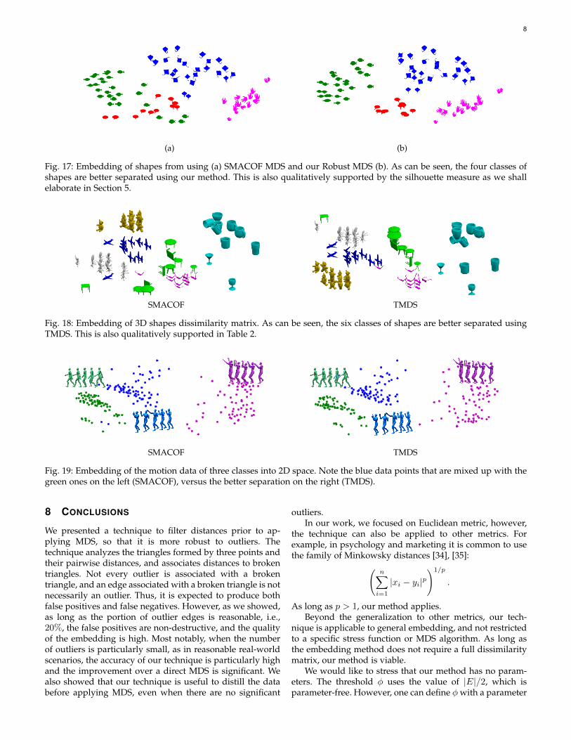
(a) (b)

Fig. 17: Embedding of shapes from using (a) SMACOF MDS and our Robust MDS (b). As can be seen, the four classes ofshapes are better separated using our method. This is also qualitatively supported by the silhouette measure as we shallelaborate in Section 5.

SMACOF TMDS

Fig. 18: Embedding of 3D shapes dissimilarity matrix. As can be seen, the six classes of shapes are better separated usingTMDS. This is also qualitatively supported in Table 2.

SMACOF TMDS

Fig. 19: Embedding of the motion data of three classes into 2D space. Note the blue data points that are mixed up with thegreen ones on the left (SMACOF), versus the better separation on the right (TMDS).

8 CONCLUSIONS

We presented a technique to filter distances prior to ap-plying MDS, so that it is more robust to outliers. Thetechnique analyzes the triangles formed by three points andtheir pairwise distances, and associates distances to brokentriangles. Not every outlier is associated with a brokentriangle, and an edge associated with a broken triangle is notnecessarily an outlier. Thus, it is expected to produce bothfalse positives and false negatives. However, as we showed,as long as the portion of outlier edges is reasonable, i.e.,20%, the false positives are non-destructive, and the qualityof the embedding is high. Most notably, when the numberof outliers is particularly small, as in reasonable real-worldscenarios, the accuracy of our technique is particularly highand the improvement over a direct MDS is significant. Wealso showed that our technique is useful to distill the databefore applying MDS, even when there are no significant

outliers.In our work, we focused on Euclidean metric, however,

the technique can also be applied to other metrics. Forexample, in psychology and marketing it is common to usethe family of Minkowsky distances [34], [35]:(

n∑i=1

|xi − yi|p)1/p

.

As long as p > 1, our method applies.Beyond the generalization to other metrics, our tech-

nique is applicable to general embedding, and not restrictedto a specific stress function or MDS algorithm. As long asthe embedding method does not require a full dissimilaritymatrix, our method is viable.

We would like to stress that our method has no param-eters. The threshold φ uses the value of |E|/2, which isparameter-free. However, one can define φwith a parameter

9

SMACOF TMDS

Fig. 20: Embedding of six classes from MPEG7 dataset. It can be seen that TMDS fixes the embedding (note the green class)but yet it is still imperfect (note the blue rooster)

SMACOF FG12 TMDS

Fig. 21: Embedding of 100 random shapes, selected from 10 classes (10 shapes per class) from the 1070db dataset. TMDSimproves the embedding compared to SMACOF (note the olive color) and FG12 (note the red and the yellow classes). Thesilhouette scores improve from 0.14 (SMACOF) and 0.19 (FG12), to 0.27 (TMDS)

SMACOF TMDS

Fig. 22: Embedding of three classes from the 1070db dataset. The gray lines present the outliers that were filtered by TMDS(44 out of 1847; that is 2.3% ). TMDS improves the embedding of the magenta and blue classes. The red circles illustrateshapes that are clearly not located close enough to the classes. Note that TMDS does not guarantee a perfect embedding.

that reflects the expected number of outliers, to refine theaccuracy of the method, i.e., to produce less false-positives.

REFERENCES

[1] J. De Leeuw, “Convergence of the majorization method for mul-tidimensional scaling,” Journal of classification, vol. 5, no. 2, pp.163–180, 1988.

[2] J. d. Leeuw and P. Mair, “Multidimensional scaling using majoriza-tion: Smacof in r,” 2008.

[3] V. De Silva and J. B. Tenenbaum, “Sparse multidimensional scalingusing landmark points,” Technical report, Stanford University,Tech. Rep., 2004.

[4] F. K. Chan and H.-C. So, “Efficient weighted multidimensionalscaling for wireless sensor network localization,” IEEE Transactionson Signal Processing, vol. 57, no. 11, pp. 4548–4553, 2009.

[5] I. Spence and S. Lewandowsky, “Robust multidimensional scal-ing,” Psychometrika, vol. 54, no. 3, pp. 501–513, 1989.

[6] P. A. Forero and G. B. Giannakis, “Sparsity-exploiting robustmultidimensional scaling,” IEEE Transactions on Signal Processing,vol. 60, no. 8, pp. 4118–4134, 2012.

[7] L. Cayton and S. Dasgupta, “Robust euclidean embedding,” inProceedings of the 23rd international conference on machine learning.ACM, 2006, pp. 169–176.

[8] J. B. Kruskal, “Nonmetric multidimensional scaling: a numericalmethod,” pp. 115–129, 1964.

[9] R. N. Shepard, “The analysis of proximities: multidimensionalscaling with an unknown distance function. i.” pp. 125–140, 1962.

[10] L. A. Neidell, “The use of nonmetric multidimensional scaling inmarketing analysis,” pp. 37–43, 1969.

[11] R. N. Shepard, “Multidimensional scaling, tree-fitting, and cluster-ing,” Science, vol. 210, no. 4468, pp. 390–398, 1980.

[12] I. Borg and P. J. Groenen, Modern multidimensional scaling: Theoryand applications. Springer Science & Business Media, 2005.

[13] A. Buja, D. F. Swayne, M. L. Littman, N. Dean, H. Hofmann,and L. Chen, “Data visualization with multidimensional scaling,”Journal of Computational and Graphical Statistics, vol. 17, no. 2, pp.444–472, 2008.

[14] A. Buja and D. F. Swayne, “Visualization methodology for mul-tidimensional scaling,” Journal of Classification, vol. 19, no. 1, pp.7–43, 2002.

[15] G. Zigelman, R. Kimmel, and N. Kiryati, “Texture mapping usingsurface flattening via multidimensional scaling,” IEEE Transactions

10

Motion Data MPEG7 3D MeshScoring SMACOF TMDS SMACOF TMDS SMACOF TMDSSilhouette 0.282 0.321 0.38 0.48 0.39 0.49Calinski Harabaz 167.2 218.9 60.54 90.5 50.7 59.0AMI 0.64 0.66 0.78 0.85 0.72 0.79Completeness 0.65 0.68 0.79 0.86 0.80 0.83Homogeneity 0.64 0.67 0.82 0.87 0.76 0.82NMI 0.65 0.674 0.81 0.86 0.78 0.82

TABLE 2: TMDS outperforms SAMCOF in the three datasets, using six common measures.

0 0.5 1 1.5 2 2.5 3 3.50

0.2

0.4

0.6

0.8

1

1.2

1.4

1.6

1.8

2

(a)

0 1 2 3 4 5 60

0.2

0.4

0.6

0.8

1

1.2

(b)

-2 -1.5 -1 -0.5 0 0.5 1 1.5 20

0.2

0.4

0.6

0.8

1

1.2

1.4

(c)

Fig. 23: The approximate normal distributions of D(p1, p2), PD, and MD are displayed in (a), (b) and (c), respectively.The green curve stands for the approximated values, while the blue, red and orange plots represent the measured distancedistributions for dimensions 6, 10, and 30, respectively. In (c) all the curves are alike, therefore we display only the oneobtained for 6D.

on Visualization and Computer Graphics, vol. 8, no. 2, pp. 198–207,2002.

[16] Z. Chen and K. Tang, “3d shape classification based on spectralfunction and mds mapping,” Journal of Computing and InformationScience in Engineering, vol. 10, no. 1, p. 011004, 2010.

[17] D. Pickup, X. Sun, P. L. Rosin, R. Martin, Z. Cheng, Z. Lian,M. Aono, A. B. Hamza, A. Bronstein, M. Bronstein et al., “Shrec14track: Shape retrieval of non-rigid 3d human models,” Proc. 3DOR,vol. 4, no. 7, p. 8, 2014.

[18] Y. Li, H. Su, C. R. Qi, N. Fish, D. Cohen-Or, and L. J. Guibas, “Jointembeddings of shapes and images via cnn image purification,”ACM Trans. Graph., vol. 34, no. 6, pp. 234:1–234:12, Oct. 2015.[Online]. Available: http://doi.acm.org/10.1145/2816795.2818071

[19] J. W. Sammon, “A nonlinear mapping for data structure analysis,”IEEE Transactions on computers, vol. 18, no. 5, pp. 401–409, 1969.

[20] J. Burkardt, CITIES - City Distance Datasets, 2011.[21] T. Denœux and M.-H. Masson, “Evclus: evidential clustering of

proximity data,” IEEE Transactions on Systems, Man, and Cybernet-ics, Part B (Cybernetics), vol. 34, no. 1, pp. 95–109, 2004.

[22] T. Graepel, R. Herbrich, P. Bollmann-Sdorra, and K. Obermayer,“Classification on pairwise proximity data,” Advances in neuralinformation processing systems, pp. 438–444, 1999.

[23] H. Ling and D. W. Jacobs, “Using the inner-distance for clas-sification of articulated shapes,” in Computer Vision and PatternRecognition, 2005. CVPR 2005. IEEE Computer Society Conference on,vol. 2. IEEE, 2005, pp. 719–726.

[24] Brown-University, 1070 Binary Shape Databases, http://vision.lems.brown.edu/content/available-software-and-databases,, 2005.

[25] X. Chen, A. Golovinskiy, and T. Funkhouser, “A benchmark for 3Dmesh segmentation,” ACM Transactions on Graphics, vol. 28, no. 3,2009.

[26] A. Aristidou, P. Charalambous, and Y. Chrysanthou, “Emotionanalysis and classification: Understanding the performers emo-tions using the LMA entities,” Computer Graphics Forum, vol. 34,no. 6, p. 262276, September 2015.

[27] Y. Kleiman, O. van Kaick, O. Sorkine-Hornung, and D. Cohen-Or,“Shed: shape edit distance for fine-grained shape similarity,” ACMTransactions on Graphics (TOG), vol. 34, no. 6, p. 235, 2015.

[28] P. J. Rousseeuw, “Silhouettes: a graphical aid to the interpretationand validation of cluster analysis,” Journal of computational andapplied mathematics, vol. 20, pp. 53–65, 1987.

[29] T. Calinski and J. Harabasz, “A dendrite method for clusteranalysis,” Communications in Statistics-theory and Methods, vol. 3,no. 1, pp. 1–27, 1974.

[30] N. X. Vinh, J. Epps, and J. Bailey, “Information theoretic measuresfor clusterings comparison: Variants, properties, normalizationand correction for chance,” Journal of Machine Learning Research,vol. 11, no. Oct, pp. 2837–2854, 2010.

[31] A. Strehl and J. Ghosh, “Cluster ensembles—a knowledge reuseframework for combining multiple partitions,” Journal of machinelearning research, vol. 3, no. Dec, pp. 583–617, 2002.

[32] A. Rosenberg and J. Hirschberg, “V-measure: A conditionalentropy-based external cluster evaluation measure.” in EMNLP-CoNLL, vol. 7, 2007, pp. 410–420.

[33] Henry, How is the distance of two random points in a unit hypercubedistributed?, 2016.

[34] Y. Zhang, J. Jiao, and Y. Ma, “Market segmentation for productfamily positioning based on fuzzy clustering,” Journal of Engineer-ing Design, vol. 18, no. 3, pp. 227–241, 2007.

[35] N. Jaworska and A. Chupetlovska-Anastasova, “A review of mul-tidimensional scaling (mds) and its utility in various psychologicaldomains,” Tutorials in Quantitative Methods for Psychology, vol. 5,no. 1, pp. 1–10, 2009.