1

Outlier detection algorithms for least squares time seriesregression1

Søren Johansen23 & Bent Nielsen4

8 September 2014

Summary: We review recent asymptotic results on some robust methods for multiple regres-sion. The regressors include stationary and non-stationary time series as well as polynomialterms. The methods include the Huber-skip M-estimator, 1-step Huber-skip M-estimators,in particular the Impulse Indicator Saturation, iterated 1-step Huber-skip M-estimators andthe Forward Search. These methods classify observations as outliers or not. From the as-ymptotic results we establish a new asymptotic theory for the gauge of these methods, whichis the expected frequency of falsely detected outliers. The asymptotic theory involves normaldistribution results and Poisson distribution results. The theory is applied to a time seriesdata set.Keywords: Huber-skip M-estimators, 1-step Huber-skip M-estimators, iteration, ForwardSearch, Impulse Indicator Saturation, Robustified Least Squares, weighted and marked em-pirical processes, iterated martingale inequality, gauge.

1 Introduction

The purpose of this paper is to review recent asymptotic results on some robust methodsfor multiple regression and apply these to calibrate these methods. The regressors includestationary and non-stationary time series as well as quite general deterministic terms. All thereviewed methods classify observations as outliers according to hard, binary decision rules.The methods include the Huber-skip M-estimator, 1-step versions such as the robustifiedleast squares estimator and the Impulse Indicator Saturation, iterated 1-step versions thereof,and the Forward Search. The paper falls in two parts. In the first part we give a motivatingempirical example. This is followed by an overview of the methods and a review of recentasymptotic tools and properties of the estimators. For all the presented methods the outlierclassification depends on a cut-off value c which is taken as given in the first part. In thesecond part we provide an asymptotic theory for setting the cut-off value c indirectly fromthe gauge, where the gauge is defined as the frequency of observations classified as outliers,when in fact there are no outliers in the data generating process.Robust methods can be used in many ways. Some methods reject observations that are

classified as outliers, while other method give a smooth weight to all observations. It is

1Acknowledgements: We would like to thank the organizers of the NordStat meeting in Turku, Finland,June 2014, for giving us the opportunity to present these lectures on outlier detection.

2The first author is grateful to CREATES - Center for Research in Econometric Analysis of Time Series(DNRF78), funded by the Danish National Research Foundation.

3Department of Economics, University of Copenhagen and CREATES, Department of Economics andBusiness, Aarhus University, DK-8000 Aarhus C. E-mail: soren.johansen@econ.ku.dk.

4Nuffi eld College & Department of Economics, University of Oxford & Programme on Economic Mod-elling, INET, Oxford. Address for correspondence: Nuffi eld College, Oxford OX1 1NF, UK. E-mail:bent.nielsen@nuffi eld.ox.ac.uk.

2

open to discussion which method to use, see for instance Hampel, Ronchetti, Rousseeuw andStahel (1986, §1.4). Here, we focus on rejection methods. We consider an empirical example,where rejection methods are useful as diagnostic tools. The idea is that most observations are‘good’in the sense that they conform with a regression model with symmetric, if not normal,errors. Some observations may not conform with the model - they are the outliers. Whenbuilding a statistical model the user can apply the outlier detection methods in combinationwith considerations about the substantive context to decide which observations are ‘good’and how to treat the ‘outliers’in the analysis.In order to use the algorithms with confidence we need to understand its properties when

all observations are ‘good’. Just as in hypothesis testing, where tests are constructed bycontrolling their properties when the hypothesis is true, we consider the outlier detectionmethods when, in fact, there are no outliers. The proposal is to control the cut-off values ofthe robust methods in terms of their gauge. The gauge is the frequency of wrongly detectedoutliers when there are none. It is distinct from, but related to, the size of a hypothesis testand of false discovery rate in multiple testing (Benjamini and Hochberg, 1995).The origins of the notion of a gauge are as follows. Hoover and Perez (1999) studied

the properties of a general-to-specific algorithm for variable selection through a simulationstudy. They considered various measures for the performance of the algorithm, that arerelated to what is now called the gauge. One of these, they referred to as the size, and thiswas the number of falsely significant variables divided by the difference between the totalnumber of variables and the number of variables with non-zero coeffi cients. The Hoover-Perezidea for regressor selection was the basis of the PcGets and Autometrics algorithms, see forinstance Hendry and Krolzig (2005), Doornik (2009) and Hendry and Doornik (2014). TheAutometrics algorithm also includes an impulse indicator saturation algorithm. Throughextensive simulation studies the critical values of these algorithms have been calibrated interms of the false detection rates for irrelevant regressors and irrelevant outliers. The termgauge was introduced in Hendry and Santos (2010) and Castle, Doornik and Hendry (2011).

Part I

Review of recent asymptotic results2 A motivating example

What is an outlier? How do we detect them? How should we deal with them? There is nosimple, universally valid answer to these questions —it all depends on the context. We willtherefore motivate our analysis with an example from time series econometrics.Demand and supply is key to discussing markets in economics. To study this Graddy

(1995, 2006) collected data on prices and quantities from the Fulton Fish market in NewYork. For our purpose the following will suffi ce. The data consists of daily data of thequantity of whiting sold by one wholesaler over the period 2 Dec 1991 to 8 May 1992. Figure1(a) shows the daily aggregated quantity Qt measured in pounds. The logarithm of thequantity, qt = logQt is shown in panel (b). The supply of fish depends on the weather at seawhere the fish is caught. Panel (c) shows a binary variable St taking value 1 if the weather

3

0 20 40 60 80 100 120

10000

20000

(a) quantities in pounds

log quantityfitted

0 20 40 60 80 100 120

7

8

9

10 (b) observations and fit

log quantityfitted

0 20 40 60 80 100 120

0.5

1.0 (c) stormy weather at sea

0 20 40 60 80 100 120

­2

0

2 (d) residuals

Figure 1: Data and properties of fitted model for Fulton Fish market data

is stormy. The present analysis is taken from Hendry and Nielsen (2007, §13.5).A simple autoregressive model for log quantities qt gives

qt(standard error)[t-statistic]

= 7.0(0.8)

[8.8]

+ 0.19(0.09)

[2.03]

qt−1 − 0.36(0.15)

[−2.39]

St, (2.1)

σ = 0.72, = −117.82, R2 = 0.090, t = 2, . . . , 111,

χ2norm[2] = 6.9 [p= 0.03], χ2skew[1] = 6.8 [p= 0.01], χ2kurt[1] = 0.04 [p= 0.84],

Far(1−2)[2, 106] = 0.9 [p= 0.40], Farch(1)[1, 106] = 1.4 [p= 0.24],

Fhet[3, 103] = 2.0 [p= 0.12], Freset[1, 106] = 1.8 [p= 0.18].

Here σ2 is the residual variance, is the log likelihood, T is the sample size. The residualspecification tests include cumulant based tests for skewness, χ2skew, kurtosis, χ

2kurtosis and

both, χ2norm = χ2skew +χ2kurtosis, a test Far for autoregressive temporal dependence, see Godfrey(1978), a test Farch for autoregressive conditional heteroscedasticity, see Engle (1982), atest Fhet for autoregressive conditional heteroscedasticity, see White (1980), and a test Fresetfor functional form, see Ramsey (1969). We note that the above references only considerstationary processes, but the specification tests also apply for non-stationary autoregressions,see Kilian and Demiroglu (2000) and Engler and Nielsen (2009) for χ2skew, χ

2kurtosis and Nielsen

(2006) for Far. The computations were done using OxMetrics, see Doornik and Hendry (2013).Figure 1(b, d) shows the fitted values and the standardized residuals.The specification tests indicate that the residuals are skew. Indeed the time series plot

of the residuals in Figure 1(d) shows a number of large negative residuals. The three largestresiduals have an interesting institutional interpretation. The observations 18 and 34 areBoxing Day and Martin Luther King Day, which are public holidays, while observation 95 isWednesday before Easter. Thus, from a substantive viewpoint it seems preferable to include

4

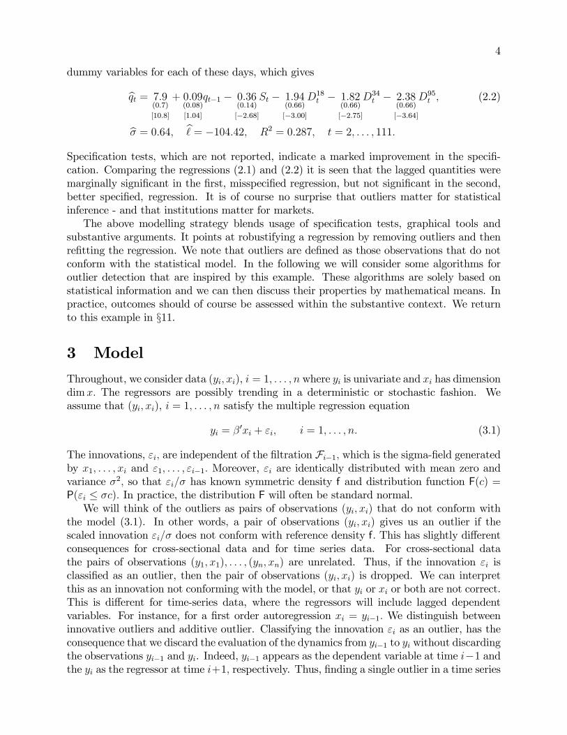
dummy variables for each of these days, which gives

qt = 7.9(0.7)

[10.8]

+ 0.09(0.08)

[1.04]

qt−1 − 0.36(0.14)

[−2.68]

St − 1.94(0.66)

[−3.00]

D18t − 1.82

(0.66)

[−2.75]

D34t − 2.38

(0.66)

[−3.64]

D95t , (2.2)

σ = 0.64, = −104.42, R2 = 0.287, t = 2, . . . , 111.

Specification tests, which are not reported, indicate a marked improvement in the specifi-cation. Comparing the regressions (2.1) and (2.2) it is seen that the lagged quantities weremarginally significant in the first, misspecified regression, but not significant in the second,better specified, regression. It is of course no surprise that outliers matter for statisticalinference - and that institutions matter for markets.The above modelling strategy blends usage of specification tests, graphical tools and

substantive arguments. It points at robustifying a regression by removing outliers and thenrefitting the regression. We note that outliers are defined as those observations that do notconform with the statistical model. In the following we will consider some algorithms foroutlier detection that are inspired by this example. These algorithms are solely based onstatistical information and we can then discuss their properties by mathematical means. Inpractice, outcomes should of course be assessed within the substantive context. We returnto this example in §11.

3 Model

Throughout, we consider data (yi, xi), i = 1, . . . , n where yi is univariate and xi has dimensiondimx. The regressors are possibly trending in a deterministic or stochastic fashion. Weassume that (yi, xi), i = 1, . . . , n satisfy the multiple regression equation

yi = β′xi + εi, i = 1, . . . , n. (3.1)

The innovations, εi, are independent of the filtration Fi−1, which is the sigma-field generatedby x1, . . . , xi and ε1, . . . , εi−1. Moreover, εi are identically distributed with mean zero andvariance σ2, so that εi/σ has known symmetric density f and distribution function F(c) =P(εi ≤ σc). In practice, the distribution F will often be standard normal.We will think of the outliers as pairs of observations (yi, xi) that do not conform with

the model (3.1). In other words, a pair of observations (yi, xi) gives us an outlier if thescaled innovation εi/σ does not conform with reference density f. This has slightly differentconsequences for cross-sectional data and for time series data. For cross-sectional datathe pairs of observations (y1, x1), . . . , (yn, xn) are unrelated. Thus, if the innovation εi isclassified as an outlier, then the pair of observations (yi, xi) is dropped. We can interpretthis as an innovation not conforming with the model, or that yi or xi or both are not correct.This is different for time-series data, where the regressors will include lagged dependentvariables. For instance, for a first order autoregression xi = yi−1. We distinguish betweeninnovative outliers and additive outlier. Classifying the innovation εi as an outlier, has theconsequence that we discard the evaluation of the dynamics from yi−1 to yi without discardingthe observations yi−1 and yi. Indeed, yi−1 appears as the dependent variable at time i−1 andthe yi as the regressor at time i+1, respectively. Thus, finding a single outlier in a time series

5

context, implies that the observations are considered correct, but possibly not generated bythe model. An additive outlier arises if an observation yi is wrongly measured. For a firstorder autoregression this is captured by two innovative outliers εi and εi+1. Discarding these,the observation yi will not appear.We consider algorithms using absolute residuals and calculation of least squares estima-

tors from selected observations. Both these choices implicitly assume a symmetric density:If non-outlying innovations were asymmetric then the symmetrically truncated innovationswould in general be asymmetric and the least squares estimator for location would be biased.With symmetry the absolute value errors |εi|/σ have density g(c) = 2f(c) and distribution

function G(c) = P(|ε1| ≤ σc) = 2F(c)− 1. We define ψ = G(c) so that c is the ψ quantile

c = G−1(ψ) = F−1{(1 + ψ)/2}, ψ ∈ [0, 1[,

while the probability of exceeding the cut-off value c is

γ = 1− ψ = 1− G(c).

Define also the truncated moments

τ =

∫ c

−cu2f(u)du, κ =

∫ c

−cu4f(u)du, κ =

∫ ∞−∞

u4f(u)du, (3.2)

and the conditional variance of ε1/σ given {|ε1| ≤ σc} as

ς2 = τ/ψ =

∫ c

−cu2f(u)du/P(|ε1/σ| ≤ c), (3.3)

which will serve as a bias correction for the variance estimators based on the truncatedsample. Define also the quantity

ζ = 2c(c2 − ς2)f(c). (3.4)

In this paper we focus on the normal reference distribution. The truncated momentsthen simplify as follows

τ = ψ − 2cf(c), κ = 3ψ − 2c(c2 + 3)f(c), κ = 3. (3.5)

4 Some outlier detection algorithms

Least squares estimators are known to be fragile with respect to outliers. A number ofrobust methods have been developed over the years. We study a variety of estimators withthe common property that outlying observations are skipped.

4.1 M-estimators

Huber (1964) introduced M-estimators as a class of maximum likelihood type estimators forlocation. The M-estimator for the regression model (3.1) is defined as the minimizer of

Rn(β) = n−1∑n

i=1ρ(yi − x′iβ). (4.1)

6

­0.2 0.0 0.2 0.4 0.6

5010

015

020

0

(a) c=1.4

0.202 0.206 0.210

28.1

5028

.165

28.1

80

(b) c=0.7

objec

tive

Figure 2: Huber-skip objective function for Fulton fish data.

for some absolutely continuous and non-negative criterion function ρ. In particular, theleast squares estimator arises when ρ(u) = u2 while the median or least absolute deviationestimator arises for ρ(u) = |u|. We will pursue the idea of hard rejection of outliers throughthe non-convex Huber-skip criterion function ρ(u) = u21(|u|≤σc) + c21(|u|>σc) for some cut-offc > 0 and known scale σ.The objective function of the Huber-skip M-estimator is non-convex. Figure 2 illustrates

the objective function for the Fish data.5 The specification is as in equation (2.1). Allparameters apart from that on qt−1 are held fixed at the values in (2.1). Panel (a) showsthat when the cut-off c is large the Huber-skip is quadratic in the central part. Panel (b)shows that when the cut-off c is smaller the objective function is non-differentiable in a finitenumber of points. Subsequently, we consider estimators that are easier to compute and applyfor unknown scale, while hopefully preserving some useful robustness properties.The asymptotic theory of M-estimators has been studied in some detail for the situation

without outliers. Huber (1964) proposed a theory for location models and convex criterionfunctions ρ. Jurecková and Sen (1996, p. 215f) analyzed the regression problem with convexcriterion functions. Non-convex criterion functions were considered for location models inJurecková and Sen (1996, p. 197f), see also Jurecková, Sen, and Picek (2012). Chen and Wu(1988) showed strong consistency of M-estimators for general criterion functions with i.i.d.ordeterministic regressors, while time series regression is analyzed in Johansen and Nielsen(2014b). We review the latter theory in §7.1.

4.2 Huber-skip estimators

We consider some estimators that involve skipping data points, but are not necessarily M-estimators. The objective functions have binary stochastic weights vi for each observation.

5Graphics were done using R 3.1.1, see R Development Core Team (2014).

7

These weights are defined in various ways below. In all cases the objective function is

Rn(β) = n−1∑n

i=1{(yi − x′iβ)2vi + c2(1− vi)}. (4.2)

The weights vi may depend on β. The first example is the Huber-skip M-estimator whichdepends on a cut-off point c, where

vi = 1(|yi−x′iβ|≤cσ). (4.3)

Another example is the Least Trimmed Squares estimator of Rousseeuw (1984) which de-pends on an integer k ≤ n, where

vi = 1(|yi−x′iβ|≤ξ(k)), (4.4)

for ξ(k) chosen as the k-th smallest order statistic of absolute residuals ξi = |yi − x′iβ| fori = 1, . . . , n. Given an integer k ≤ n we can find ψ and c so k/n = ψ = G−1(c), and ψ, c, kare different ways of calibrating the methods. In either case, once the regression estimatorβ has been determined the scale can be estimated by

σ2 = ς−2(∑n

i=1vi)−1{∑n

i=1vi(yi − x′iβ)2}, (4.5)

where ς2 = τ/ψ is the consistency correction factor defined in (3.3).For the Least Trimmed Squares estimator it holds that

∑ni=1(1− vi) = n− k. Thus, the

last term in the objective function (4.2) does not depend on β, so that it is equivalent tooptimize

Rn,LTS(β) = n−1n∑i=1

vi(yi − x′iβ)2. (4.6)

The Least Trimmed Squares weight (4.4) is scale invariant in contrast to the Huber-skipM-estimator. It is known to have breakdown point of γ = 1− ψ = 1− k/n for ψ < 1/2, seeRousseeuw and Leroy (1987, §3.4). An asymptotic theory is provided by Víšek (2006a,b,c).The estimator is computed through a binomial search algorithm which is uncomputable inmost practical situations, see Maronna, Martin and Yohai (2006, §5.7) for a discussion. Anumber of iterative approximations have been suggested such as the Fast LTS algorithm byRousseeuw and van Driessen (1998). This leaves additional questions with respect to theproperties of the approximating algorithms.If the weights vi do not depend on β, the objective function has a least squares solution

β = (∑n

i=1vixix′i)−1(∑n

i=1vixiyi). (4.7)

From this the variance estimator (4.5) can be computed. Examples include 1-step Huber-skipM-estimators based on initial estimators β, σ2, where

vi = 1(|yi−x′iβ|≤cσ), (4.8)

and 1-step Huber-skip L-estimators based on an initial estimator β and a cut-off k < n,which defines the k-th smallest order statistic ξ(k) of absolute residuals ξi = |yi−x′iβ|, where

vi = 1(|yi−x′iβ|≤ξ(k)). (4.9)

8

These estimators are computationally attractive, but require a good starting point. Theycan also be iterated. As before, we see that the 1-step L-estimator does not require an initialscale estimator in contrast to the 1-step M-estimator.Robustified least squares arises if the initial estimators β, σ2 are the full-sample least

squares estimators. This relates to the estimation procedure for the Fulton Fish Marketdata in §2. This approach can be fragile, especially when there are more than a few outliers,see Welsh and Ronchetti (2002) for a discussion.The 1-step estimators relate to the 1-step M-estimators of Bickel (1975), although he was

primarily concerned with smooths weights vi. His idea was to apply preliminary estimatorsβ(0), (σ(0))2 and then define the 1-step estimator β(1) by linearising the first order condition.He also suggested iteration, but no results were given.Ruppert and Carroll (1980) studied a related 1-step L-estimator for which fixed propor-

tions of negative and positive residuals are skipped. Following their suggestion we refer tothe estimator with weights (4.9) as a 1-step Huber-skip L-estimator, because the objectivefunction is defined by weights involving an order statistics. We note that there is a mismatchin the nomenclature of L and M-estimators. Jaeckel (1971) defined L-estimators for locationproblems in terms of the estimator, whereas Huber (1964) defined M-estimators in terms ofthe objective function. Thus, the Least Trimmed Squares estimator is not classified as anL-estimator, although its objective function is a quadratic combination of order statistics.

4.3 Some statistical algorithms

We give three statistical algorithms involving iteration of 1-step Huber-skip estimators.These are the iterated 1-step Huber-skip M-estimator, the Impulse Indicator Saturation,and the Forward Search.The 1-step Huber-skip estimators are amenable to iteration. Here we consider iterated

Huber-skip M-estimators.

Algorithm 4.1 Iterated 1-step Huber-skip M-estimator. Choose a cut-off c > 0.1. Choose initial estimators β(0), (σ(0))2 and let m = 0.

2. Define indicator variables v(m)i as in (4.8), replacing β, σ2 by β(m), (σ(m))2.3. Compute least squares estimators β(m+1), (σ(m+1))2 as in (4.7), (4.5) replacing vi by v

(m)i .

4. Let m = m+ 1 and repeat 2 and 3.

The Iteration Algorithm 4.1 does not have a stopping rule. This leaves the questionswhether the algorithm convergences with increasing m and n and in which sense it approxi-mates the Huber-skip estimator.The Impulse Indicator Saturation algorithm has its roots in the empirical work of Hendry

(1999) and Hendry, Johansen and Santos (2008). It is a 1-step M-estimator, where theinitial estimator is formed by exploiting in a simple way the assumption, that a subset ofobservations is free of outliers. The idea is to divide the sample into two sub-samples. Thenrun a regression on each sub-sample and use this to find outliers in the other sub-sample.

Algorithm 4.2 Impulse Indicator Saturation. Choose a cut-off c > 0.1.1. Split indices in sets Ij, for j = 1, 2, of nj observations.

9

1.2. Calculate the least squares estimators for (β, σ2) based upon sample Ij as

βj = (∑

i∈Ijxix′i)−1(∑

i∈Ijxiyi), σ2j =1

nj

∑i∈Ij(yi − x

′iβj)

2.

1.3. Define indicator variables for each observation

v(−1)i = 1(i∈I1)1(|yi−x′iβ2|≤cσ2)

+ 1(i∈I2)1(|yi−x′iβ1|≤cσ1), (4.10)

1.4. Compute least squares estimators β(0), (σ(0))2 using (4.7), (4.5), replacing vi by v(−1)i

and let m = 0.2. Define indicator variables v(m)i = 1(|yi−x′iβ(m)|≤cσ(m))

as in (4.8).

3. Compute least squares estimators β(m+1), (σ(m+1))2 as in (4.7), (4.5), replacing vi by v(m)i .

4. Let m = m+ 1 and repeat 2 and 3.

Due to its split half approach to the initial estimation, the Impulse Indicator Satura-tion may be more robust than robustified least squares. The Impulse Indicator Saturationestimator will work best when the outliers are known to be in a particular subset of theobservations. For instance, consider the split half case where index sets I1, I2 are chosen asthe first half and the second half of the observations, respectively. Then the algorithm has agood ability to detect for instance a level shift half way through the second sample, while itis poor at detecting outliers scattered throughout both samples, because both sample halvesare contaminated. If the location of the contamination is unknown, one will have to iterateover the choice of the initial sets I1, I2. This is what the more widely used Autometricsalgorithm does, see Doornik (2009) and Doornik and Hendry (2014).The Forward Search algorithm is an iterated 1-step Huber-skip L-estimator suggested

for the multivariate location model by Hadi (1992) and for multiple regression by Hadi andSimonoff (1993) and developed further by Atkinson and Riani (2000), see also Atkinson,Riani and Cerioli (2010). The algorithm starts with a robust estimate of the regressionparameters. This is used to construct the set of observations with the smallest m0 absoluteresiduals. We then run a regression on thosem0 observations and compute absolute residualsof all n observations. The observations with m0 + 1 smallest residuals are then selected, anda new regression is performed on these m0 + 1 observations. This is then iterated. Sincethe estimator based on the m0 + 1 observation is computed in terms of the order statisticbased on the estimator for the m0 observation, it is a 1-step Huber-skip L-estimator. Wheniterating the order of the order statistics is gradually expanding.

Algorithm 4.3 Forward Search.1. Choose an integer m0 < n and an initial estimators β(m0), and let m = m0.2.1. Compute absolute residuals ξ(m)i = |yi − x′iβ(m)| for i = 1, . . . , n.

2.2. Find the (m+ 1)th smallest order statistic z(m) = ξ(m)(m+1).

2.3. Define indicator variables v(m)i = 1(|yi−x′iβ(m)|≤ξ

(m)(m+1)

)as in (4.9).

3. Compute least squares estimators β(m+1), (σ(m+1))2 as in (4.7), (4.5) replacing vi by v(m)i .

4. If m < n let m = m+ 1 and repeat 2 and 3.

10

The Forward Search Algorithm 4.3 has a finite number of steps. It terminates whenm = n − 1 and β(n), (σ(n))2 are the full sample least squares estimators. Applying thealgorithm form = m0, . . . , n−1, results in sequences of least squares estimators β(m), (σ(m))2

and order statistics z(m) = ξ(m)(m+1).

The idea of the Forward Search is to monitor the plot of scaled forward residuals z(m)/σ(m).For each m we can find the asymptotic distribution of z(m)/σ(m) and add a curve of point-wise p-quantiles as a function of m for some p. The first m for which z(m)/σ(m) exceeds thequantile curve is the estimate m of the number of non-outliers. Asymptotic theory for theforward residuals z(m)/σ(m) is reviewed in §8.3. A theory for the estimator m is given in §10.A variant of the Forward Search advocated by Atkinson and Riani (2000) is to use the

minimum deletion residuals d(m) = mini 6∈S(m) ξ(m)i instead of the forward residuals z(m).

5 Overview of the results for the location case

We give an overview of the asymptotic theory for the M-type Huber-skip estimators for thelocation problem, where x′iβ reduces to a location parameter µ. The theory evolves aroundtwo asymptotic results. The first is an asymptotic distribution for the M-estimator. Thesecond is an asymptotic expansion for 1-step M-estimators. The iterated 1-step M-estimatorsare found to converge to the M-estimator.Huber (1964) proposed an asymptotic theory for M-estimators with convex objective

function in location models. His proof did not extend to the Huber-skip M-estimator basedon the weights (4.3). Instead he assumed consistency and conjectured that the asymptoticdistribution would be, for symmetric f,

n1/2(µ− µ) =1

ψ − 2cf(c)n−1/2

∑ni=1εi1(|εi|≤σc) + oP(1)

D→ N[0,τσ2

{ψ − 2cf(c)}2 ]. (5.1)

This result is generalized to time series regression in Theorem 7.1.In the situation with normal errors τ = ψ − 2cf(c), see (3.5), the asymptotic variance in

(5.1) reduces to σ2/τ. The effi ciency relative to the sample average, which is the least squaresestimator, is therefore τ. The bottom curve plotted in Figure 3 shows the effi ciency as afunction of ψ. The least trimmed squares estimator has the same asymptotic distribution.Next, consider the 1-step Huber-skip M-estimator based on weights (4.8). It has asymp-

totic expansion linking the updated estimator µ(1) with the initial estimator µ(0) through

n1/2(µ(1) − µ) =1

ψn−1/2

∑ni=1εi1(|εi|≤σc) +

2cf(c)

ψn1/2(µ(0) − µ) + oP(1), (5.2)

see Theorem 7.2 for regression.Robustified least squares arises, if we choose the initial estimator µ(0) as the least squares

estimator. In that case we get the expansion

n1/2(µ(1) − µ) =1

ψn−1/2

∑ni=1εi1(|εi|≤σc) +

2cf(c)

ψn−1/2

∑ni=1εi + oP(1). (5.3)

We can use the Central Limit Theorem to show asymptotic normality of the estimator.The asymptotic variance follows in Theorem 7.3. The effi ciency relative to least squaresestimation is shown as the top curve in Figure 3.

11

0.0 0.5 1.0 1.5 2.0 2.5 3.0

0.0

0.2

0.4

0.6

0.8

1.0

cut­off value c

effi

cien

cy

robustified least squares =Impulse Indicator Saturation, m=0Impulse Indicator Saturation, m=1Huber­skip M­estimator

Figure 3: The effi ciency of robustified least squares, the Impulse Indicator Saturation, andthe Huber-skip M-estimator relative to full sample least squares when the reference distrib-ution is normal.

Starting with other estimators give different asymptotic variances. An example is theImpulse Indicator Saturation Algorithm 4.2. Theorem 7.4 shows that the initial split-halfestimator µ(0) has the same asymptotic distribution as the robustified least squares estimator.The updated 1-step estimator µ(1) is slightly less effi cient, as shown by the middle curve inFigure 3, but hopefully more robust.The 1-step M-estimator can be iterated along the lines of Algorithm 4.1. This iteration

has a fixed point µ∗ solving the equation

n1/2(µ∗ − µ) =1

ψn−1/2

∑ni=1εi1(|εi|≤σc) +

2cf(c)

ψn1/2(µ∗ − µ) + oP(1), (5.4)

see Theorem 7.6. Thus, any influence of the initial estimator is lost through iteration. Solvingthis equation gives

n1/2(µ∗ − µ) =1

ψ − 2cf(c)

∑ni=1εi1(|εi|≤σc) + oP(1), (5.5)

with the same leading term as the Huber-skip M-estimator in (5.1).

6 Preliminary asymptotic results

We present the main ingredient for the asymptotic theory.

6.1 Assumptions on regressors and density

The innovations εi and regressors xi must satisfy moment assumptions. The innovations εihave symmetric density with derivative satisfying boundedness and tail conditions. Related

12

conditions on the density are often seen in the literatures on empirical processes and quantileprocesses. These conditions are satisfied for the normal distribution and t-distributions,see Johansen and Nielsen (2014a) for a discussion. For the iterated estimator we need anassumption of unimodality. The minimal assumptions vary for the different estimators,as explored in Johansen and Nielsen (2009, 2013, 2014a, 2014b) for 1-step Huber-skip M-estimators, for iterated 1-step Huber-skip M-estimators, for the Forward Search and forgeneral M-estimators, respectively.For this presentation we simply assume a normal reference distribution, which, of course,

is most used in practice. With normality we avoid a somewhat tedious discussion of existenceof moments of a certain order. The regressors can be temporally dependent and possiblydeterministically or stochastically trending.

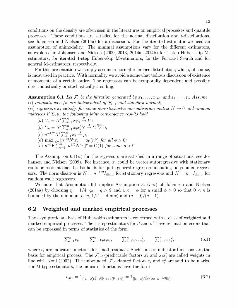
Assumption 6.1 Let Fi be the filtration generated by x1, . . . , xi+1 and ε1, . . . , εi. Assume(i) innovations εi/σ are independent of Fi−1 and standard normal;(ii) regressors xi satisfy, for some non-stochastic normalisation matrix N → 0 and randommatrices V,Σ, µ, the following joint convergence results hold

(a) Vn = N ′∑n

i=1 xiεiD→ V ;

(b) Σn = N ′∑n

i=1 xix′iN

D→ Σa.s.> 0;

(c) n−1/2N ′∑n

i=1 xiD→ µ;

(d) maxi≤n |n1/2N ′xi| = oP(nφ) for all φ > 0;(e) n−1E

∑ni=1 |n1/2N ′xi|q = O(1) for some q > 9.

The Assumption 6.1(ii) for the regressors are satisfied in a range of situations, see Jo-hansen and Nielsen (2009). For instance, xi could be vector autoregressive with stationaryroots or roots at one. It also holds for quite general regressors including polynomial regres-sors. The normalisation is N = n−1/2Idimx for stationary regressors and N = n−1Idimx forrandom walk regressors.We note that Assumption 6.1 implies Assumption 3.1(i, ii) of Johansen and Nielsen

(2014a) by choosing η = 1/4, q0 = q > 9 and a κ = φ for a small φ > 0 so that 0 < κ isbounded by the minimum of η, 1/(1 + dimx) and (q − 9)/(q − 1).

6.2 Weighted and marked empirical processes

The asymptotic analysis of Huber-skip estimators is concerned with a class of weighted andmarked empirical processes. The 1-step estimators for β and σ2 have estimation errors thatcan be expressed in terms of statistics of the form∑n

i=1vi,∑n

i=1vixiεi,∑n

i=1vixix′i,

∑ni=1viε

2i , (6.1)

where vi are indicator functions for small residuals. Such sums of indicator functions are thebasis for empirical process. The Fi−1-predictable factors xi and xix′i are called weights inline with Koul (2002). The unbounded, Fi-adapted factors εi and ε2i are said to be marks.For M-type estimators, the indicator functions have the form

vM,i = 1{|εi−x′i(β−β)|≤σc+(σ−σ)c}= 1{|εi−x′iNb|≤σc+n−1/2ac}

, (6.2)

13

which allows for estimation uncertainty b = N−1(β−β) and a = n1/2(σ−σ) in the regressioncoeffi cient β and in the scale σ. For L-type estimators the indicators are

vL,i = 1{|εi−x′i(β−β)|≤ξ(k)}= 1{|εi−x′iNb|≤σ(c+n−1/2d)}

, (6.3)

which allows for estimation uncertainty b = N−1(β − β) and d = n1/2(ξ/σ − c) in theregression coeffi cient β and in the quantile ξ.We will need an asymptotic linearization of the statistics (6.1) with respect to the esti-

mation uncertainty. For this purpose we start by considering weights

vb,c,di = 1{|εi−x′iNb|≤σ(c+n−1/2d)}, (6.4)

where the estimation uncertainty is replaced by bounded, deterministic terms b, d. Subse-quently, we apply the result to M-type and L-type estimators, by replacing b by b and d byac/σ and d, respectively.The following asymptotic expansion is a version of Lemma D.5 of Johansen and Nielsen

(2014a) formulated under the present simplified Assumption 6.1.

Theorem 6.1 (Johansen and Nielsen, 2014a, Lemma D.5) Suppose Assumption 6.1 holds.Consider the product moments (6.1) with weights vb,c,di given by (6.4) and expansions

n−1/2∑n

i=1vb,c,di = n−1/2

∑ni=11(|εi|≤σc) + 2f(c)d+Rv(b, c, d),

n−1/2∑n

i=1vb,c,di ε2i = n−1/2

∑ni=1ε

2i 1(|εi|≤σc) + 2σ2c2f(c)d+Rvεε(b, c, d),

N ′∑n

i=1vb,c,di xiεi = N ′

∑ni=1xiεi1(|εi|≤σc) + 2cf(c)N ′

∑ni=1xix

′iNb+Rvxε(b, c, d),

N ′∑n

i=1vb,c,di xix

′iN = ψN ′

∑ni=1xix

′iN +Rvxx(b, c, d).

LetR(b, c, d) = |Rv(b, c, d)|+ |Rvεε(b, c, d)|+ |Rvxε(b, c, d)|+ |Rvxx(b, c, d)|

Then it holds for all (large) B > 0, all (small) η > 0 and n→∞ that

sup|b|,|d|≤n1/4−ηB

sup0<c<∞

R(b, c, d) = oP(1). (6.5)

In particular, for bounded c, then

sup|a|,|b|≤n1/4−ηB

sup0<c≤B

R(b, c, ac/σ) = oP(1). (6.6)

Theorem 6.1 is proved by a chaining argument. The idea is to cover the domain of b, dwith a finite number of balls. The supremum over the large compact set can then be replacedby considering the maximum value over the centers of the balls and the maximum of thevariation within balls. By subtracting the compensators of the product moments we turnthem into martingales. The argument will therefore be a consideration of the tail behaviourof the maximum of a family of martingales using the iterated martingale inequality presentedin §6.3 and Taylor expansions of the compensators.Related results of Theorem 6.1 are considered in the literature. Koul and Ossiander

(1994) considered weighted empirical processes without marks and with η > 1/4. Johansenand Nielsen (2009) considered the situation (6.6) for fixed c and with η > 1/4.

14

6.3 An iterated martingale inequality

We present an iterated martingale inequality, which can be used to assess the tail behaviourof the maximum of a family of martingales. It builds on an exponential martingale inequalityby Bercu and Touati (2008).

Theorem 6.2 (Bercu and Touati, 2008, Theorem 2.1) For i = 1, . . . , n let (mi,Fi) be alocally square integrable martingale difference. Then, for all x, y > 0,

P[|∑n

i=1mi| ≥ x,∑n

i=1{m2i + E(m2

i |Fi−1)} ≤ y] ≤ 2 exp(−x2

2y).

In order to bound a family of martingales it is useful to iterate this martingale inequalityto get the following iterated martingale inequality.

Theorem 6.3 (Johansen and Nielsen, 2014a, Theorem 5.2.) For ` = 1, . . . , L let z`,i beFi-adapted so Ez2

r

`,i <∞ for some r ∈ N. Let Dr = max1≤`≤L∑n

i=1E(z2r

`,i|Fi−1) for 1 ≤ r ≤ r.Then, for all κ0, κ1, . . . , κr > 0, it holds

P[ max1≤`≤L

|∑n

i=1{z`,i − E(z`,i|Fi−1)}| > κ0] ≤ LEDr

κr+∑r

r=1

EDr

κr+ 2L

∑r−1r=0 exp(− κ2r

14κr+1).

Theorem 6.3 contains parameters κ0, κ1, . . . , κr, which can be chosen in various ways. Wegive two examples taken from Theorems 5.3, 5.4 of Johansen and Nielsen (2014a)The first example is to show that the remainder terms in Theorem 6.1 are uniformly

small. In the proof we consider a family of size L = O(nλ) where λ > 0 depends on thedimension of the regressor and seek to prove that the maximum of the family of martingalesis of order oP(n1/2). Choosing κq = (κn1/2)2

q(28λ log n)1−2

q, so that κ2q/κq+1 = 28λ log n and

κ0 = κn1/2, a result of that type follows.The second example is to show that the empirical processes (6.1) are tight. In this case

the family is of fixed size L, and now the probability that the maximum of the family ofmartingales is larger than κn1/2 has to be bounded by a small number. Choosing κq =κn2

q−1θ1−2

qso κ2q/κq+1 = κθ and κ0 = κn1/2 a result of that type follows.

7 Asymptotic results for Huber-skip M-estimators

We consider recent results on the Huber-skip M-estimator as well as for 1-step Huber-skipM-estimators and iterations thereof.

7.1 Huber-skip M-estimators

The Huber-skip M-estimator is the solution to the optimization problem (4.2) with weights(4.3). Since this problem is non-convex we need an additional assumption that boundsthe frequency of small regressors. That bound involves a function that is an approximateinverse of the function λn(α) appearing in the analysis of S-estimators by Davies (1990), seealso Chen and Wu (1988). The bound can be satisfied for stationary and non-stationary

15

regressors. The condition is used to prove that the objective function is uniformly boundedbelow for large values of the parameter, a property that implies existence and tightness ofthe estimator. For full descriptions of the bound to the regressors and extensions to a widerclass of M-estimators, see Johansen and Nielsen (2014b).

Theorem 7.1 (Johansen and Nielsen, 2014b, Theorems 1,2,3) Consider the Huber-skip M-estimator defined from (4.2), (4.3). Suppose Assumption 6.1 holds and that the frequency ofsmall regressors is bounded as outlined above. Then any minimizer of the objective function(4.2) has a measurable version and satisfies

N−1(β − β) =1

ψ − 2cf(c)Σ−1n N ′

∑ni=1xiεi1(|εi|≤σc) + oP(1).

If, in addition the regressors are stationary then

n1/2(β − β)D→ N{0,Σ−1σ2/τ}.

Theorem 7.1 proves the conjecture (5.1) of Huber (1964) for time series regression. Theregularity conditions on the regressors are much weaker than those normally considered infor instance Chen and Wu (1988), Liese and Vajda (1994), Maronna, Martin, and Yohai(2006), Huber and Ronchetti (2009), and Jurecková, Sen, and Picek (2012). Theorem 7.1extends to non-normal, but symmetric densities and even to non-symmetric densities andobjective function, by introducing a bias correction.Theorem 7.1 is proved in three steps. First, it is shown that β is tight, that isN−1(β−β) =

OP(n1/2), through a geometric argument that requires the assumption to the frequency ofsmall regressors. Secondly, it is shown that β is consistent, in the sense that N−1(β − β) =OP(n1/2−τ ) for any τ < 1/4, using the iterated martingale inequality of Theorem 6.3. Finally,the presented expansion of Theorem 7.1 is proved, again using Theorem 6.3.

7.2 1-step Huber-skip M-estimators

The asymptotic theory of the 1-step Huber-skip M-estimator for regression is given in Jo-hansen and Nielsen (2009). The main result is a stochastic expansion of the updated esti-mation error in terms of a kernel and the original estimation error. It follows from a directapplication of Theorem 6.1.

Theorem 7.2 (Johansen and Nielsen, 2009, Corollary 1.2) Consider the 1-step Huber-skipM-estimators β(1), σ(1) defined by (4.7), (4.5) with weights (4.8). Suppose Assumption 6.1holds and that N−1(β(0) − β) and n1/2(σ(0) − σ) are OP(1). Then

N−1(β(1) − β) =1

ψΣ−1n N ′

∑ni=1xiεi1(|εi|≤σc) +

2cf(c)

ψN−1(β(0) − β) + oP(1). (7.1)

n1/2(σ(1) − σ) =1

2τσn−1/2

∑ni=1(ε

2i − σ2

τ

ψ)1(|εi|≤σc) +

ζ

2τn1/2(σ(0) − σ) + oP(1) (7.2)

16

Theorem 7.2 generalises the statement (5.2) for the location problem. Theorem 7.2 showsthat the updated regression estimator β(1) only depends on the initial regression estimatorβ(0) and not on the initial scale estimator σ(0). This is a consequence of the symmetry imposedon the problem. Johansen and Nielsen (2009) also analyze situations where the referencedistribution f is non-symmetric and the cut-off is made in a matching non-symmetric way.In that situation both expansions involve the initial estimation uncertainty for β and σ2.We can immediately use Theorem 7.2 for an m-fold iteration of (7.1), (7.2). Results for

infinite iterations follow in §7.5.

7.3 Robustified Least Squares

Robustified least squares arises when the initial estimators are the full-sample least squaresestimator. We can analyze this 1-step Huber-skip M-estimator using Theorem 7.2. Theproduct moment properties in Assumption 6.1 imply that the initial estimators satisfy

N−1(β − β) = OP(1), n1/2(σ2 − σ2) = n−1/2∑n

i=1(ε2i − σ2) + OP(n−1/2). (7.3)

Thus, the conditions of Theorem 7.2 are satisfied so that the robustified least squares esti-mators can be expanded as in (7.1), (7.2). The asymptotic distribution of estimator for βwill depend on the properties of the regressors. For simplicity the regressors are assumedstationary in the following result.

Theorem 7.3 (Johansen and Nielsen, 2009, Corollary 1.4) Consider the 1-step Huber-skipM-estimator defined with the weights (4.8) and where the initial estimators β, σ2 are thefull-sample least squares estimators. Suppose Assumption 6.1 holds and that the regressorsare stationary. Then

n1/2(

β − βσ2 − σ2

)D→ N

{0,

(σ2ηβΣ−1 0

0 2σ4ησ

)},

where, using the coeffi cients (τ,κ, ζ) from (3.2) and (3.4), the effi ciency factors ηβ, ησ are

ψ2ηβ = τ{1 + 4cf(c)}+ {2cf(c)}2, 2τ 2ησ = (κ − τ 2/ψ)(1 + ζ) +ζ2

4(κ− 1). (7.4)

The result generalises the statement (5.3) for the location problem. The effi ciency factorηβ is plotted as the top curve in Figure 3. A plot of the effi ciency for the variance, ησ can befound in Johansen and Nielsen (2009, Figure 1.1). Situations with non-stationary regressorsare also discussed in that paper.

7.4 Impulse Indicator Saturation

Impulse Indicator Saturation is a second example of a 1-step Huber-skip M-estimator. Thisrequires the choice of sub-samble Ij, each with nj observations. If the product momentproperties of Assumption 6.1 hold for each sub-sample and nj/n → λj > 0 then the initialestimators satisfy

N−1(βj − β) = OP(1), n1/2j (σ2 − σ2) = n

−1/2j

∑i∈Ij(ε

2i − σ2) + OP(n−1/2). (7.5)

17

The asymptotic distribution theory will depend on the choice of sub-samples and regressors.For simplicity we only report the split-half case with subsets I1 = (i ≤ n/2) and I2 = (i >n/2) and stationary regressors.

Theorem 7.4 (Johansen and Nielsen, 2009, Theorems 1.5, 1.7) Consider the split-half Im-pulse Indicator Saturation estimator of Algorithm 4.2. Suppose Assumption 6.1 holds withstationary regressors. Recall the effi ciency factors ηβ, ησ from (7.4). Then the initial esti-mators satisfy

n1/2{

β(0) − β(σ(0))2 − σ2

}D→ N

{0,

(σ2ηβΣ−1 0

0 2σ4ησ

)},

Moreover, the updated Impulse Indicator Saturation estimator satisfies

n1/2(β(1) − β)D→ N(0, σ2ηiisβ Σ−1),

whereψ4ηiisβ = {ψ + 2cf(c)}τ [ψ + 2cf(c) + 2{2cf(c)}2] +

1

2{2cf(c)}4.

The effi ciency factors ηβ and ηiisβ for the split-half case are plotted as the top and themiddle curve, respectively, in Figure 3. Johansen and Nielsen (2009) also discuss situationswith general index sets I1, I2 and where the regressors are non-stationary.

7.5 Iterated 1-step Huber-skip M-estimators

The asymptotic theory of the iterated 1-step Huber-skip M-estimator for regression is givenin Johansen and Nielsen (2013). This includes iteration of the robustified least squaresestimator and of the Impulse Indicator Saturation estimator with general index sets andgeneral regressors. In each step the asymptotic theory is governed by Theorem 7.2. Butwhat does it take to control the iteration and establish a fixed point result?We start by showing that the sequence of normalised estimators β(m), σ(m) is tight.

Theorem 7.5 (Johansen and Nielsen, 2013, Theorem 3.3) Consider the iterated 1-stepHuber-skip M-estimator in Algorithm 4.1. Suppose Assumption 6.1 holds and that N−1(β(0)−β) and n1/2(σ(0) − σ) are OP(1). Then

sup0≤m<∞

|N−1(β(m) − β)|+ |n1/2(σ(m) − σ)| = OP(1).

Theorem 7.5 is proved by showing that the expansions (7.1), (7.2) are contractions.Necessary conditions are that 2cf(c)/ψ < 1 and ζ/(2τ) < 1. This holds for normal or t-distributed innovations, see Johansen and Nielsen (2013, Theorem 3.6).In turn, Theorem 7.5 leads to a fixed point result for infinitely iterated estimators.

Theorem 7.6 (Johansen and Nielsen, 2013, Theorem 3.3) Consider the iterated 1-stepHuber-skip M-estimator in Algorithm 4.1. Suppose Assumption 6.1 holds and that N−1(β(0)−

18

β) and n1/2(σ(0) − σ) are OP(1). Then, for all ε, η > 0 a pair m0, n0 > 0 exists so for allm > m0 and n > n0 it holds

P{|N−1(β(m) − β∗)|+ n1/2|σ(m) − σ∗| > η} < ε,

where

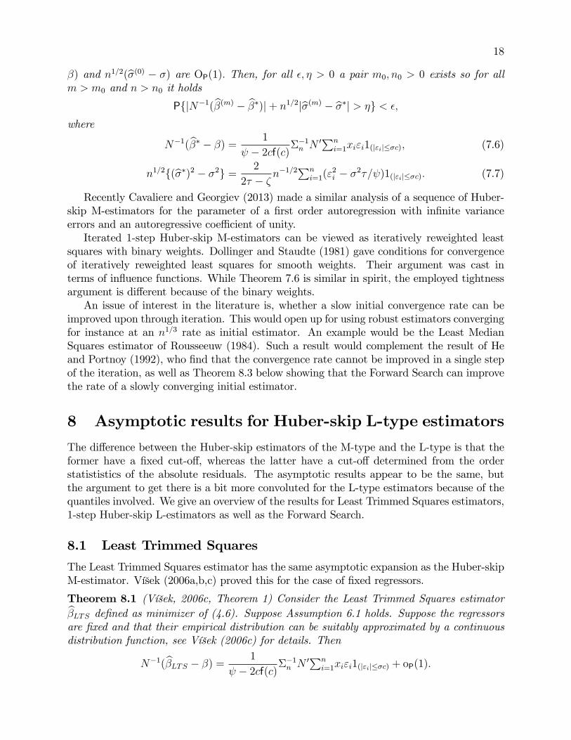
N−1(β∗ − β) =1

ψ − 2cf(c)Σ−1n N ′

∑ni=1xiεi1(|εi|≤σc), (7.6)

n1/2{(σ∗)2 − σ2} =2

2τ − ζ n−1/2∑n

i=1(ε2i − σ2τ/ψ)1(|εi|≤σc). (7.7)

Recently Cavaliere and Georgiev (2013) made a similar analysis of a sequence of Huber-skip M-estimators for the parameter of a first order autoregression with infinite varianceerrors and an autoregressive coeffi cient of unity.Iterated 1-step Huber-skip M-estimators can be viewed as iteratively reweighted least

squares with binary weights. Dollinger and Staudte (1981) gave conditions for convergenceof iteratively reweighted least squares for smooth weights. Their argument was cast interms of influence functions. While Theorem 7.6 is similar in spirit, the employed tightnessargument is different because of the binary weights.An issue of interest in the literature is, whether a slow initial convergence rate can be

improved upon through iteration. This would open up for using robust estimators convergingfor instance at an n1/3 rate as initial estimator. An example would be the Least MedianSquares estimator of Rousseeuw (1984). Such a result would complement the result of Heand Portnoy (1992), who find that the convergence rate cannot be improved in a single stepof the iteration, as well as Theorem 8.3 below showing that the Forward Search can improvethe rate of a slowly converging initial estimator.

8 Asymptotic results for Huber-skip L-type estimators

The difference between the Huber-skip estimators of the M-type and the L-type is that theformer have a fixed cut-off, whereas the latter have a cut-off determined from the orderstatististics of the absolute residuals. The asymptotic results appear to be the same, butthe argument to get there is a bit more convoluted for the L-type estimators because of thequantiles involved. We give an overview of the results for Least Trimmed Squares estimators,1-step Huber-skip L-estimators as well as the Forward Search.

8.1 Least Trimmed Squares

The Least Trimmed Squares estimator has the same asymptotic expansion as the Huber-skipM-estimator. Víšek (2006a,b,c) proved this for the case of fixed regressors.

Theorem 8.1 (Víšek, 2006c, Theorem 1) Consider the Least Trimmed Squares estimatorβLTS defined as minimizer of (4.6). Suppose Assumption 6.1 holds. Suppose the regressorsare fixed and that their empirical distribution can be suitably approximated by a continuousdistribution function, see Víšek (2006c) for details. Then

N−1(βLTS − β) =1

ψ − 2cf(c)Σ−1n N ′

∑ni=1xiεi1(|εi|≤σc) + oP(1).

19

8.2 1-step Huber-skip L-estimators

The 1-step Huber-skip L-estimator has the following expansion.

Theorem 8.2 Consider the 1-step Huber-skip L-estimators β(1), σ(1) defined by (4.7), (4.5)with weights (4.9). Suppose Assumption 6.1 holds and that N−1(β(0) − β) is OP(1). Then

N−1(β(1) − β) =1

ψΣ−1n N

∑ni=1xiεi1(|εi|≤σc) +

2cf(c)

ψN−1(β(0) − β) + oP(1). (8.1)

n1/2(σ(1) − σ) =1

2τσn−1/2

∑ni=1(ε

2i − σ2

τ

ψ)1(|εi|≤σc) +

ζ

2τn1/2(

ξ(k)c− σ) + oP(1) (8.2)

=1

2τσn−1/2

∑ni=1(ε

2i − σ2

τ

ψ)1(|εi|≤σc) +

σζ

4cτn−1/2

∑ni=1{1(|εi|≤σc) − ψ}+ oP(1)

(8.3)

Proof. Equations (8.1), (8.2) follow from Theorem 6.1. Equation (8.3) with its expansionof the quantile ξ(k) follows from Johansen and Nielsen (2014a, Lemma D.11).

Ruppert and Carroll (1980) state a similar result for a related 1-step L-estimator, butomit the details of the proof. It is interested to note that the expansions of the one-stepregression estimator of L-type in (8.1) is the same as for the M-type in (7.1). In contrast, thevariance estimators have different expansions. In particular, the L-estimator does not usethe initial variance estimator and, consequently, the expansion does not involve uncertaintyfrom the initial estimation.

8.3 Forward Search

The Forward Search is an iterated 1-step Huber-skip L-estimator, where the cut-off changesslightly in each step. We highlight asymptotic expansions for the forward regression estima-tors β(m) and for the scaled forward residuals z(m)/σ(m). The results are formulated in termsof embeddings of the time series β(m), σ(m), z(m) for m = m0 + 1, . . . , n into the space D[0, 1]of right continuous functions with limits from the left, for instance,

βψ =

{β(m) for m = integer(nψ) and ψ0 = m0/n ≤ ψ ≤ 1,0 otherwise.

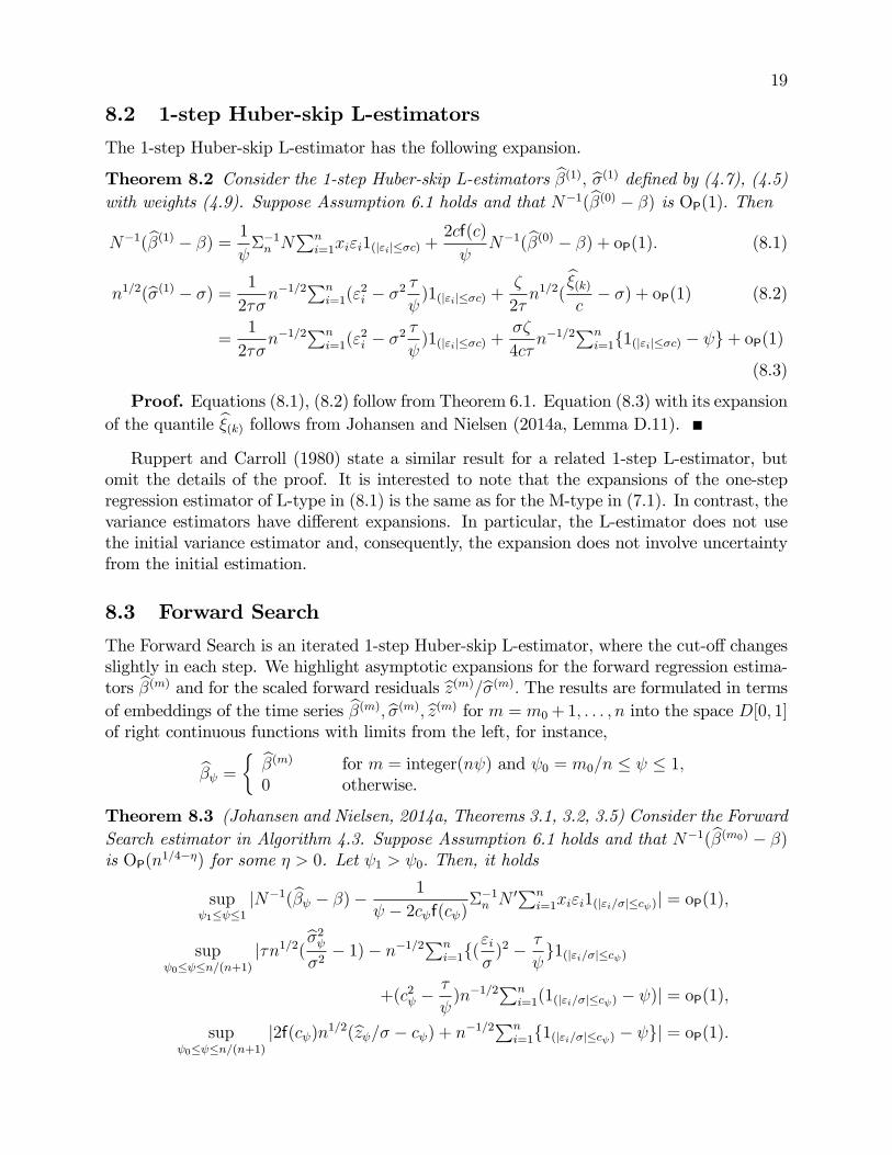
Theorem 8.3 (Johansen and Nielsen, 2014a, Theorems 3.1, 3.2, 3.5) Consider the ForwardSearch estimator in Algorithm 4.3. Suppose Assumption 6.1 holds and that N−1(β(m0) − β)is OP(n1/4−η) for some η > 0. Let ψ1 > ψ0. Then, it holds

supψ1≤ψ≤1

|N−1(βψ − β)− 1

ψ − 2cψf(cψ)Σ−1n N ′

∑ni=1xiεi1(|εi/σ|≤cψ)| = oP(1),

supψ0≤ψ≤n/(n+1)

|τn1/2(σ2ψσ2− 1)− n−1/2

∑ni=1{(

εiσ

)2 − τ

ψ}1(|εi/σ|≤cψ)

+(c2ψ −τ

ψ)n−1/2

∑ni=1(1(|εi/σ|≤cψ) − ψ)| = oP(1),

supψ0≤ψ≤n/(n+1)

|2f(cψ)n1/2(zψ/σ − cψ) + n−1/2∑n

i=1{1(|εi/σ|≤cψ) − ψ}| = oP(1).

20

The asymptotic variances and covariances are given in Theorem A.1.

The proof uses the theory of weighted and marked empirical processes outlined in §6.2combined with the theory of quantile processes discussed in Csörgo (1983). A single step ofthe algorithm was previously analyzed in Johansen and Nielsen (2010).Comparing Theorem 8.3 with Theorems, 7.6, 8.1, we recognise the asymptotic result for

the estimator for β. The effi ciency relative to the least squares estimator is shown as the bot-tom curve in Figure 3. The asymptotic expansion for the variance estimator σ2ψ is, however,different from the expression for the iterated 1-step Huber-skip M-estimator in Theorem7.6, reflecting the different handling of the scale. The Bahadur (1966) representation link-ing the empirical distribution of the scaled innovations εi/σ with their order statistics, cψsay, implies that 2f(cψ)n1/2(zψ/σ − cψ) vanishes. Moreover, the minimum deletion residuald(m) = mini 6∈S(m) ξ

(m)i has the same asymptotic expansion as z(m) = ξ

(m)(m+1) after a burn-in

period. See Johansen and Nielsen (2014a, Theorem 3.4) for details.The idea of the Forward Search is to monitor the plot of the sequence of scaled forward

residuals. Combining the expansions for σψ and zψ in Theorem 8.3 gives the next result.

Theorem 8.4 (Johansen and Nielsen 2014a, Theorem 3.3). Consider the Forward Search-estimator in Algorithm 4.3. Suppose Assumption 6.1 holds and that N−1(β(m0) − β) isOP(n1/4−η) for some η > 0. Let ψ1 > ψ0. Then

supψ0≤ψ≤n/(n+1)

|2f(cψ)n1/2(zψσψ− cψ) + Zn(cψ)| = oP(1),

where the process Zn(c) given by

{1− cψf(cψ)

τ(c2ψ −

τ

ψ)}n−1/2

∑ni=1{1(|εi/σ|≤c) − ψ}+

cψf(cψ)

τn−1/2

∑ni=1{(

εiσ

)2 − τ

ψ}1(|εi/σ|≤c)

(8.4)converges to a Gaussian process Z. The covariance of Z is given in Theorem A.1.

Part II

Gauge as a measure of false detectionWe now present some new results for the outlier detection algorithms. Outlier detectionalgorithms will detect outliers with a positive probability when in fact there are no outliers. xxxWe analyze this in terms of the gauge, which is the expected frequency of falsely detectedoutliers when, in fact, the data generating process has no outliers. The idea of a gaugeoriginates in the work of Hoover and Perez (1999) and is formally introduced in Hendry andSantos (2010), see also Castle, Doornik and Hendry (2011).The gauge concept is related to, but also distinct from the concept of a size of a statistical

test, which is the probability of falsely rejecting a true hypothesis. For a statistical test wechoose the critical value indirectly from the size we are willing to tolerate. In the same way,for an outlier detection algorithm, we can choose the cut-off for outliers indirectly from thegauge we are willing to tolerate.

21

The detection algorithms assign binary weigths vi to each observation, so that vi = 0 foroutliers and vi = 1 otherwise. We define the empirical or sample gauge as the frequency offalsely detected outliers

γ =1

n

∑ni=1(1− vi). (8.5)

In turn, the population gauge is the expected frequency of falsely detected outliers, when infact the model has no contamination, that is

Eγ = E1

n

∑ni=1(1− vi).

To see how the gauge of an outlier detection algorithm relates to the size of a statisticaltest, consider an outlier detection algorithm which classify observations as outliers if theabsolute residuals |yi − x′iβ|/σ is large for some estimator (β, σ). That algorithm has gauge

γ =1

n

∑ni=1(1− vi) =

1

n

∑ni=11(|yi−x′iβ|>σc)

. (8.6)

Suppose the parameters β, σ where known so that we could choose β, σ as β, σ. Then thepopulation gauge reduces to the size of a test that a single observation is an outlier, that is

E1

n

∑ni=11(|yi−x′iβ|>σc) = E

1

n

∑ni=11(|εi|>σc) = P(|ε1| > σc) = γ.

In general, the population gauge will, however, be different from the size of such a testbecause of the estimation error. In §9, §10 we analyze the gauge implicit in the definition ofa variety of estimators of type M and L, respectively. Proofs follow in the appendix.

9 The gauge of Huber-skip M-estimators

Initially a consistency result is given for the gauge of Huber-skip M-estimators and a distrib-ution theory follows. A normal theory arises when the proportion of falsely detected outliersis controlled by fixing the cut-off c as n increases whereas a Poisson exceedence theory ariseswhen nγ is held fixed as n increases.

9.1 Asymptotic analysis of the gauge

We give an asymptotic expansion of the sample gauge of the type (8.6).

Theorem 9.1 Consider a sample gauge γ of the form (8.6). Suppose Assumption 6.1 holdsand that N−1(β − β), n1/2(σ2 − σ2) are OP(1). Then, for fixed c,

n1/2(γ − γ) = n−1/2∑n

i=1{1(|εi|>σc) − γ}+ 2cf(c)n1/2(σ

σ− 1) + oP(1). (9.1)

It follows that Eγ → γ.

22

Note that convergence in mean is equivalent to convergence in probability since the gaugetakes values in the interval [0, 1], see Billingsley (1968, Theorem 5.4).Theorem 9.1 applies to various Huber-skip M-estimators. For the Huber-skip M-estimator

the estimators β, σ2 are the Huber-skip estimator and corresponding variance estimator. For1-step Huber-skip M-estimator the estimators β, σ2 are the initial estimators. For ImpulseIndicator Saturation or 1-step Huber-skip M-estimator iterated m times the estimators β, σ2

are the estimators from step m− 1.

9.2 Normal approximations to gauge

We control the proportion of falsely discovered outliers by fixing the cut-off c. In that case anasymptotically normal distribution theory follows from the expansion in Theorem 9.1. Theasymptotic variance is analyzed case by case since the expansion in Theorem 9.1 dependson the variance estimator σ2.Huber-skip M-estimator: Theorem 7.1 shows thatN−1(β−β) is tight. This is the simplest

case to analyse since the variance is assumed known so that σ2 = σ2. Therefore only the firstbinomial term in Theorem 9.1 matters.

Theorem 9.2 Consider the Huber-skip M-estimator β defined from (4.2), (4.3) with knownσ, fixed c and sample gauge γ = n−1

∑ni=11(|yi−x′iβ|>σc)

. Suppose Assumption 6.1 holds. Then

n1/2(γ − γ)D→ N{0, γ(1− γ)}.

The robustified least squares estimator: This is the 1-step Huber-skip M-estimator βdefined in (4.7), (4.8), where the initial estimators β, σ2 are the full-sample least squaresestimators. The binomial term in Theorem 9.1 is now combined with a term from the initialvariance estimator σ2.

Theorem 9.3 Consider the robustified least squares estimator β defined from (4.7), (4.8),and the initial estimators β and σ2 are the full sample least squares estimators, fixed c andsample gauge is γ = n−1

∑ni=11(|yi−x′iβ|>σc)

. Suppose Assumption 6.1 holds. Then

n1/2(γ − γ)D→ N[0, γ(1− γ) + 2cf(c)(τ − ψ) + {cf(c)}2(κ− 1)].

The variance in Theorem 9.3 is larger than the binomial variance for a normal referencedistribution and any choice of γ. This is seen through differentiation with respect to c.The split-half Impulse Indicator Saturation estimator: The estimator is defined in Algo-

rithm 4.2. Initially, the outliers are defined using the indicator v(−1)i based on the split-sampleestimators β1, σ21 and β2, σ

22, see (4.10). The outliers are reassessed using the updated esti-

mators β(0), σ(0). Thus, the algorithm gives rise to two sample gauges

γ(−1) = n−1∑

i∈I11(|yi−x′iβ2|>σ2c)+ n−1

∑i∈I21(|yi−x′iβ1|>σ1c)

, (9.2)

γ(0) = n−1∑n

i=11(|yi−x′iβ(0)|>σ(0)c). (9.3)

For simplicity we only report the result for the initial gauge γ(−1). The updated gauge γ(0)

has a different asymptotic variance.

23

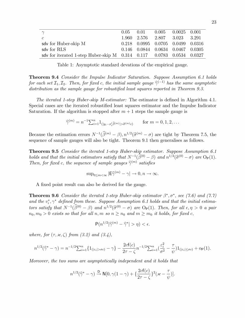
γ 0.05 0.01 0.005 0.0025 0.001c 1.960 2.576 2.807 3.023 3.291sdv for Huber-skip M 0.218 0.0995 0.0705 0.0499 0.0316sdv for RLS 0.146 0.0844 0.0634 0.0467 0.0305sdv for iterated 1-step Huber-skip M 0.314 0.117 0.0783 0.0534 0.0327

Table 1: Asymptotic standard devations of the empirical gauge.

Theorem 9.4 Consider the Impulse Indicator Saturation. Suppose Assumption 6.1 holdsfor each set I1, I2. Then, for fixed c, the initial sample gauge γ(−1) has the same asymptoticdistribution as the sample gauge for robustified least squares reported in Theorem 9.3.

The iterated 1-step Huber-skip M-estimator: The estimator is defined in Algorithm 4.1.Special cases are the iterated robustified least squares estimator and the Impulse IndicatorSaturation. If the algorithm is stopped after m+ 1 steps the sample gauge is

γ(m) = n−1∑n

i=11(|yi−x′iβ(m)|>σ(m)c)for m = 0, 1, 2, . . .

Because the estimation errors N−1(β(m) − β), n1/2(σ(m) − σ) are tight by Theorem 7.5, thesequence of sample gauges will also be tight. Theorem 9.1 then generalises as follows.

Theorem 9.5 Consider the iterated 1-step Huber-skip estimator. Suppose Assumption 6.1holds and that the initial estimators satisfy that N−1(β(0)− β) and n1/2(σ(0)− σ) are OP(1).Then, for fixed c, the sequence of sample gauges γ(m) satisfies

sup0≤m<∞ |Eγ(m) − γ| → 0, n→∞.

A fixed point result can also be derived for the gauge.

Theorem 9.6 Consider the iterated 1-step Huber-skip estimator β∗, σ∗, see (7.6) and (7.7)and the v∗i , γ

∗ defined from these. Suppose Assumption 6.1 holds and that the initial estima-tors satisfy that N−1(β(0) − β) and n1/2(σ(0) − σ) are OP(1). Then, for all ε, η > 0 a pairn0,m0 > 0 exists so that for all n,m so n ≥ n0 and m ≥ m0 it holds, for fixed c,

P(n1/2|γ(m) − γ∗| > η) < ε.

where, for (τ,κ, ζ) from (3.2) and (3.4),

n1/2(γ∗ − γ) = n−1/2∑n

i=1{1(|εi|>σc) − γ} −2cf(c)

2τ − ζ n−1/2∑n

i=1(ε2iσ2− τ

ψ)1(|εi|≤σc) + oP(1).

Moreover, the two sums are asymptotically independent and it holds that

n1/2(γ∗ − γ)D→ N[0, γ(1− γ) + { 2cf(c)

2τ − ζ }2(κ − τ

ψ)].

24

Table 1 shows the asymptotic variances for the Huber-skip M-estimator, the RobustifiedLeast Squares and for the fully iterated 1-step Huber-skip estimators . The latter includeiterated Robustified Least Squares and iterated Impulse Indicator Saturation. The resultsare taken from Theorems 9.2, 9.3, 9.6, respectively. For gauges of 1% or lower the standarddeviations are very similar. If the gauge is chosen as γ = 0.05 and n = 100, then the samplegauges γ will be asymptotically normal with mean γ = 0.05 and a standard deviation ofabout 0.2/n1/2 = 0.02. This suggests that it is not unusual to find up to 8-9 outliers when infact there are none. Lowering the gauge to γ = 0.01 or γ = 0.0025, the standard deviationis about 0.1/n1/2 = 0.01 and 0.05/n1/2 = 0.005, respectively, when n = 100. Thus, it is notunusual to find up to 2-3 and up to 1 outliers, respectively, when in fact there are none. Thissuggests that the gauge should be chosen rather small in line with the discussion in Hendryand Doornik (2014, §7.6).

9.3 Poisson approximation to gauge

If we set the cut-off so as to accept the same fixed number λ of falsely discovered outliersregardless of the sample size, then a Poisson exceedence theory arises.The idea is to choose the cut-off cn so that, for some λ > 0,

P(|εi| > σcn) = λ/n. (9.4)

The cut-off cn appears both in the definition of the gauge and in the definition of theestimators, so some care is needed. We build the argument around the 1-step M-estimator.Let βn and σn be sequences of estimators that may depend on cn, hence the subscript n inthe notation for the estimators. Given these estimators, the sample gauge is

γn = n−1∑n

i=11(|yi−x′iβn|>σncn). (9.5)

In the first result we assume that estimation errors N−1(βn − β) and n1/2(σn − σ) aretight. Thus, the result immediately applies to robustified least squares, where the initialestimators βn and σn are the full sample least squares estimators, which do not depend onthe cut-off cn. But, in general we need to check this tightness condition.

Theorem 9.7 Consider the 1-step Huber-skip M-estimator, where nP (|ε1| ≥ σcn) = λ.Suppose Assumption 6.1 holds, and that N−1(βn−β) and n1/2(σ2n−σ2) are OP(1). Then thesample gauge γn in (9.5) satisfies

nγnD→ Poisson(λ).

We next discuss this result for particular initial estimators.Robustified least squares estimator: The initial estimators β and σ2 are the full sample

least squares estimators. These do not depend on cn so Theorem 9.7 trivially applies.

Theorem 9.8 Consider the robustified least squares estimator β defined from (4.7), (4.8),where the initial estimators β and σ2 are the full sample least squares estimators, whilecn is defined from (9.4). Suppose Assumption 6.1 holds. Then the sample gauge γn =n−1∑n

i=11(|yi−x′iβ|>σcn)satisfies

nγnD→ Poisson(λ).

25

xλ cn=100 cn=200 0 1 2 3 4 55 1.960 2.241 0.01 0.04 0.12 0.27 0.44 0.621 2.576 2.807 0.37 0.74 0.92 0.98 1.000.5 2.807 3.023 0.61 0.91 0.98 1.000.25 3.023 3.227 0.78 0.97 1.000.1 3.291 3.481 0.90 1.00

Table 2: Poisson approximations to the probability of finding at most x outliers for a givenλ. The implied cut-off cn = Φ−1{1− λ/(2n)} is shown for n = 100 and n = 200.

Impulse Indicator Saturation: Let βj and σ2j be the split sample least squares estimators.These do not depend on cn so Theorem 9.7 trivially applies for the split sample gauge basedon

v(−1)i,n = 1(i∈I1)1(|yi−x′iβ2|>σ2cn)

+ 1(i∈I2)1(|yi−x′iβ1|>σ1cn).

The updated estimators β(0)n and (σ(0)n )2 do, however, depend on the cut-off. Thus, an

additional argument is needed, when considering the gauge based on the combined initialestimator as in

v(0)i,n = 1

(|yi−x′iβ(0)n |>σ(0)n cn)

.

Theorem 9.9 Consider the Impulse Indicator Saturation Algorithm 4.2. Let cn be definedfrom (9.4). Suppose Assumption 6.1 holds for each set I1, I2. Let the estimators β(0)n and(σ(0)n )2 be defined from (4.7), (4.5) replacing vi by v

(−1)i,n . Then N−1(β(0)n −β) and n1/2(σ(0)n −σ)

are OP(1), and

nγ(m)n =∑n

i=1(1− v(m)i,n )

D→ Poisson(λ) for m = −1, 0.

Table 1 shows the Poisson approximation to the probability of finding at most x outliersfor different values of λ. For small λ and n this approximation is possibly more accuratethan the normal approximation, although that would have to be investigated in a detailedsimulation study. The Poisson distribution is left skew so the probability of finding at mostx = λ outliers increases from 62% to 90% for λ decreasing from 5 to 0.1. In particular, forλ = 1 and n = 100 so the cut-off is cn = 2.58 the probability of finding at most one outlier is74% and the probability of finding at most two outliers is 92%. In other words, the chanceof finding 3 or more outliers is small when in fact there are none.

10 The gauge of Huber-skip L-type estimators

We now consider the gauge for the L-type estimators. The results and their consequences aresomewhat different from the results for M-type estimators. For the Least Trimmed Squaresestimator the gauge is trivially γ = γ, because the purpose of the estimator is to keep thetrimming proportion fixed. For the Forward Search the idea is to stop the algorithm oncethe forward residuals z(m)/σ(m) become too big. We develop a stopping rule from the gauge.

26

10.1 Gauge for the Forward Search

The forward plot of forward residuals consists of the scaled forward residuals z(m)/σ(m)

for m = m0, . . . , n − 1. Along with this we plot point-wise confidence bands derived fromTheorem 8.4. Suppose we define some stopping time m based on this information, so that mis the number of non-outlying observations while n− m is the number of the outliers. Thisstopping time can then be calibrated in terms of the sample gauge (8.5), which simplifies as

γ =n− mn

=1

n

∑n−1m=m0

(n−m)1(m=m).

Rewrite this by substituting n−m =∑n−1

j=m 1 and change order of summation to get

γ =1

n

∑n−1j=m0

1(m≤j). (10.1)

If the stopping time is an exit time, then the event (m ≤ j) is true if z(m)/σ(m) has exitedat the latest by m = j.An example of a stopping time is the following. Theorem 8.4 shows that

Zn(cψ) = 2f(c)n1/2(zψσψ− cψ) = Zn(cψ) + oP(1) (10.2)

uniformly in ψ0 ≤ ψ ≤ n/(n + 1), where Zn converges to a Gaussian process Z. We nowchoose the stopping time as the first time greater than or equal to m1(≥ m0), z

(m)/σ(m)

exceeds some constant level q times its pointwise asymptotic standard deviation, that is,

m = arg minm1≤m<n

[Zn(cm/n) > qsdv{Zn(cm/n)}]. (10.3)

To analyze the stopping time (10.3) we consider the event (m ≤ j). This event satisfies

(m ≤ j) = [ maxm1≤m≤j

Zn(cm/n)

sdv{Zn(cm/n)}> q].

Inserting this expression into (10.1) and then using expansion (10.2) we arrive at the followingresult, with details given in the appendix.

Theorem 10.1 Consider the Forward Search. Suppose Assumption 6.1 holds. Let m0 =int(ψ0n) and m1 = int(ψ1n) for some ψ1 ≥ ψ0 > 0. Consider the stopping time m in (10.3)for some c ≥ 0. Then

Eγ = En− mn

→ γ =

∫ 1

ψ1

P[ supψ1≤ψ≤u

Z(cψ)

sdv{Z(cψ)} > q]du.

If ψ1 > ψ0, the same limit holds for the forward search when replacing z(m) by the deletionresidual d(m) in the definition of m in (10.3).

27

γ vs ψ1 0.05 0.10 0.20 0.30 0.40 0.50 0.60 0.70 0.80 0.900.10 2.50 2.43 2.28 2.14 1.99 1.81 1.60 1.31 0.82 -0.05 2.77 2.71 2.58 2.46 2.33 2.19 2.02 1.79 1.45 0.690.01 3.30 3.24 3.14 3.04 2.94 2.83 2.71 2.55 2.33 1.910.005 3.49 3.44 3.35 3.26 3.15 3.04 2.95 2.81 2.62 2.260.001 3.90 3.85 3.77 3.69 3.62 3.53 3.43 3.32 3.18 2.92

Table 3: Cut-off values q for Forward Search as a function of gauge γ and lower point ψ1 ofrange for the stopping time.

The integral in Theorem 10.1 cannot be computed analytically in an obvious way. In-stead we simulated it using Ox 7, see Doornik (2007). For a given n, draws of normalεi can be made. From this, the process Zn in (8.4) can be computed. The maximum ofZn(cm/n)/sdv{Z(cm/n)} over m1 ≤ m ≤ j can then be computed for any m1 ≤ j ≤ n.Repeating this nrep times the probability appearing as the integrand can be estimated for agiven value of q and u . From this the integral γ can be computed. This expresses γ = γ(ψ1, q)as a function of q and ψ1. Inverting this for fixed ψ1 expresses q = q(ψ1, γ) as a function ofγ and ψ1. Results are reported in the Table 3 for nrep = 105 and n = 1600.

11 Application to fish data

11.1 Impulse Indicator Saturation

The Impulse Indicator Saturation of Algorithm 4.2 is an iterative procedure. Assuminginnovations are normal cut-offs can be chosen according to a standard normal distribution.For a finite iteration, where the number of steps is chosen apriori, this follows from Theorem9.1. For an infinite iteration, this follows from Theorem 9.6. Thus, the cut-off is 2.58 for a1% gauge. When applying the procedure we split the sample in the first and last half.The estimated model for the first sample half is

q(1st half)t = 6.5

(1.1)+ 0.26(0.12)

qt−1 − 0.51(0.18)

St, σ = 0.66, t = 2, . . . , 56.

The preliminary second half outliers are in observations 95, 108, 68, 75, 94 with residuals−4.66, −3.11, −2.85, −2.74, −2.66. The estimated model for the second sample half is

q(2nd half)t = 7.5

(1.2)+ 0.13(0.14)

qt−1 − 0.21(0.30)

St, σ = 0.77, t = 57, . . . , 111.

The preliminary first half outliers are in observations 18, 34 with residuals −3.78, −2.95.In step m = 0 we estimate a model with dummies for the preliminary outliers and get

the full sample model

q(0)t = − 1.98

(0.60)

[−3.16]

D18t − 1.80

(0.61)

[−2.93]

D34t − 1.26

(0.60)

[−2.10]

D68t − 1.34

(0.60)

[−2.23]

D75t − 1.35

(0.60)

[−2.25]

D94t − 2.40

(0.61)

[−3.96]

D95t

− 1.56(0.60)

[−2.61]

D108t + 7.8

(0.7)+ 0.11(0.08)

qt−1 − 0.41(0.13)

St, σ = 0.60,

28

with standardised coeffi cients reported in square brackets. The observations 18, 34, 95, 108remain outliers. All residuals - for observations without indicators - are now smaller thanthe cut-off value. Thus we conclude that the observations 18, 34, 95, 108 are outliers.In step m = 1 we get the Impulse Indicator Saturation model

q(1)t = − 1.96

(0.63)

[−3.10]

D18t − 1.82

(0.65)

[−2.81]

D34t − 2.40

(0.64)

[−3.76]

D95t − 1.55

(0.63)

[−2.44]

D108t

+ 7.9(0.7)

+ 0.09(0.08)

qt−1 − 0.39(0.14)

St, σ = 0.63.

The observations 18, 34, 95 remain outliers, while all residuals are small.In step m = 2 the estimated model is identical to the model (2.2). In that model the

observations 18, 34, 95 remain outliers, while all residuals are smaller. Thus, the algorithmhas reached a fixed point.If the gauge is chosen as 0.5% or 0.25% so the cut-off is 2.81 or 3.02, respectively, the

algorithm will converge to a solution taking 18, 95 or 95 as outliers, respectively.

11.2 Forward Search

We need to choose the initial estimator, the fractions ψ0, ψ1 and the gauge. As initial estima-tor we chose the fast LTS estimator by Rousseeuw and van Driessen (1998) as implementedin the ltsReg function of the R-package robustbase. We chose to use it with breakdownpoint 1 − ψ0. There is no asymptotic analysis of this estimator. It is meant to be an ap-proximation to the Least Trimmed Squares estimator, for which we have Theorem 8.1 basedon Vícek (2006c). That result requires fixed regressors. Nonetheless, we apply it to the fishdata where the two regressors are the lagged dependent variable and the binary variable Stwhich is an indicator for stormy weather. We choose ψ0 = ψ1 as either 0.95 or 0.8.Figure 4 shows the forward plots of the forward residuals ξ(m)(m+1)/ςm/nσ

(m+1), where thescaling is chosen in line with Atkinson, Riani and Cerioli (2010). Consider panel (a) whereψ0 = ψ1 = 0.95. Choose the gauge as, for instance, γ = 0.01, in which case the we needto consider the third exit band from the top. This is exceeded for m = 107, pointing atn − m = 3 outliers. These are the three holiday observations 18, 34, 95 discussed in §2. Ifthe gauge is set to γ = 0.001 we find no outliers. If the gauge is set to γ = 0.05 we findm = 104, pointing at n− m = 6, which is 5% of the observations.Consider now panel (b) where ψ0 = ψ1 = 0.80.With a gauge of γ = 0.01 we find m = 96,

pointing at n − m = 14 outliers. These include the three holiday observations along with11 other observations. This leaves some uncertainty about the best choice of the numberof outliers. The present analysis is based on asymptotics and could be distorted in finitesamples.

12 Conclusion and further work

The results presented concern the asymptotic properties of a variety of Huber-skip estimatorsin the situation where there are no outliers, and the reference distribution is symmetric if

29

104 105 106 107 108 109 110

2.4

2.6

2.8

3.0

3.2

3.4

(a) ψ0=ψ1=0.95

90 95 100 105 110

2.0

2.5

3.0

(b) ψ0=ψ1=0.80

forw

ard 

resi

dual

Figure 4: Forward Plots of forward residuals for fish data. Here ψ0 = ψ1 is chosen either as0.95 or 0.80. The bottom curve shows the pointwise median. The top curves show the exitbands for gauges chosen as, from top, 0.001, 0.005, 0.01, 0.05, respectively. Panel (b) alsoincludes an exit band for a gauge of 0.10.

not normal. Combined with the concept of the gauge, these results are used for calibratingthe cut-off values of the estimators.In further research we will look at situations, where there actually are outliers. Various

configurations of outliers will be of interest: single outliers, clusters of outliers, level shifts,symmetric and non-symmetric outliers. The probability of finding particular outliers is calledpotency in Hendry and Santos (2010). It will then be possible to compare the potency oftwo different outlier detection algorithms, that are calibrated to have the same gauge.The approach presented is different from the traditional approaches of robust statistics.

It would be of interest to compare the approach with the traditional idea of analyzing robustestimators in terms of their breakdown point, see Hampel (1971), or the influence function,see Hampel, Ronchetti, Rousseeuw and Stahel (1986) or Maronna, Martin and Yohai (2006).First order asymptotic theory is known to be fragile in some situations. A comprehensive

simulation study of the results presented would therefore be useful, possibly building onAtkinson and Riani (2006) and Hendry and Doornik (2014).It would be of interest to extend this research to variable selection algorithms such as

Autometrics, see Hendry and Doornik (2014). The Impulse Indicator Saturation is a stylizedversion of Autometrics. It should work well, if the researcher can identify a part of the data,that is free from outliers. If this is not the case, one will have to iterate over the choiceof sub-samples. In Autometrics potential outliers are coded as dummy variables and thealgorithm then searches over these dummy variables along with the other regressors.

30

A Proofs

For the asymptotic normality results for the gauge some covariance matrices have to becomputed. The results are collected in

Theorem A.1 Suppose Assumption 6.1 holds and that c = G(ψ). Then the processes

An(c) = n−1/2∑n

i=1{1(|εi|>σc) − γ},

Bn(c) = n−1/2∑n

i=1(ε2iσ2− τ

ψ)1(|εi|≤σc),

Cn(c) = n−1/2∑n

i=1(ε2iσ2− 1),

Kn(c) = N ′∑n

i=1xiεi1(|εi/σ|≤c)

converge to continuous limits A,B,C,K on D[0, 1] endowed with the uniform metric. Theprocesses An,Bn,Cn have Gaussian limits with covariance matrix

Φ = V ar

An(c)Bn(c)Cn(c)

=

γ(1− γ) 0 τ − ψ

0 κ − τ 2/ψ κ − τ 2/ψτ − ψ κ − τ 2/ψ (κ− 1)/2

. (A.1)

If the regressors are stationary, then K is Gaussian independent of A,B,C with varianceτσ2Σ.It follows that the asymptotic variance in Theorem 8.3 is given by

asVar

{2f(cψ)n1/2(zψ/σ − cψ)n1/2(σ2ψ/σ

2 − 1)

}= Var

{An(cψ)

Bn(cψ)/τ + (c2ψ/τ − 1/ψ)An(cψ)

}= ω′1Φω1

for

ω′1 =

(1 0 0

(c2ψ/τ − 1/ψ) 1/τ 0

).

The asymptotic variance in Theorem 8.4 is given by

asV ar(2f(cψ)n1/2(zψ/σψ − cψ)

= V ar(−{1− cψf(cψ)

τ(c2ψ −

τ

ψ)}An(cψ) +

cψf(cψ)

τBn(cψ)) = ω′2Φω2

whereω′2 =

(−{1− cψf(cψ)

τ(c2ψ − τ

ψ)}, cψf(cψ)

τ, 0

).

Proof of Theorem 9.1. Apply the asymptotic expansion in Theorem 6.1.

Proof of Theorem 9.2. Insert σ2 = σ2 in the expansion in Theorem 9.1 and applyTheorem A.1 to the binomial term.

31

Proof of Theorem 9.3. The initial estimators satisfyN−1(β−β) = OP(1) and n1/2(σ2−σ2) = n−1/2

∑ni=1(ε

2i − σ2) + oP(1), see (7.3). Use Theorem 9.1 to get

n1/2(γ − γ) = n−1/2∑n

i=1{1(|εi|>σc) − γ}+ cf(c)n−1/2∑n

i=1(ε2i − σ2) + oP(1), (A.2)

and apply Theorem A.1.

Proof of Theorem 9.4. The initial estimators satisfy N−1(βj − β) = OP(1) andn1/2(σ2j − σ2) = n−1/2

∑ni=1(ε

2i − σ2) + oP(1), see (7.5). Insert this in the expansion in

Theorem 9.1 to get

n−1/2j

∑i∈Ij{1(|yi−x′iβ3−j |>σ3−jc)−γ} = n

−1/2j

∑i∈Ij{1(|εi|>σc)−γ}+cf(c)n

−1/2j

∑i∈Ij(ε

2i−σ2)+oP(1).

Combine the counts of outliers for the two sub-samples to get

n1/2(γ(−1) − γ) = n−1/2∑2

j=1

n1/2j

n1/2j

∑i∈Ij{1(|yi−x′iβ3−j |>σ3−jc) − γ}

= n−1/2∑2

j=1

∑i∈Ij{1(|εi|>σc) − γ}+ cf(c)n−1/2

∑2j=1

∑i∈Ij(ε

2i − σ2) + oP(1).

This is reduces to the expansion (A.2) for the robustified least squares estimator.

Proof of Theorem 9.5. Theorem 7.5 shows that the normalised estimators are tight.Thus, for all ε there exists an A > 0 so that the set

An =⋂∞m=0{|N−1(β(m) − β)|+ |n1/2{(σ(m))2 − σ2}| ≤ U} (A.3)

has probability of at least 1− ε. Theorem 6.1 then shows that on that set

γ(m) − γ =1

n

∑ni=1{1(|εi|>σc) − γ} − n−1/22cf(c)n1/2(σ(m)/σ − 1) + oP(n−1/2), (A.4)

where, uniformly inm, the first term and the second term are OP(n−1/2), while the remainderterm is oP(n−1/2). Therefore

sup0≤m<∞ |γ(m) − γ| = oP(1).

Since γ(m) and γ are bounded by one then E sup0≤m<∞ |γ(m)− γ| vanishes as n→∞. Thus,by the triangle inequality

sup0≤m<∞ |Eγ(m) − γ| ≤ sup0≤m<∞ E|γ(m) − γ| ≤ E sup0≤m<∞ |γ(m) − γ| = o(1).

Proof of Theorem 9.6. On the set An defined in the proof of Theorem 9.5, see (A.3),we consider the expansion (A.4), that is,

n1/2(γ(m) − γ) = n−1/2∑n

i=1{1(|εi|>σc) − γ} − 2cf(c)n1/2(σ(m)/σ − 1) + oP(1),

32

where the remainder is uniform in m. Theorem 7.6 shows that for large m,n we have

n1/2(σ(m)/σ − 1) =1

2τ − ζ n−1/2∑n

i=1(ε2iσ2− τ

ψ)1(|εi|≤σc) + oP(1),

where the remainder is uniform inm. Combine to get the desired expansion. The asymptoticnormality follows from Lemma A.1.

Theorem 9.7 is a special case of the following Lemma subjected to Remarks A.1 and A.2below, because Assumption 6.1 assumes Gaussian errors.

Lemma A.2 Suppose Assumption 6.1(ii, d) holds. Let the cut-off cn be given by (9.4) andassume that(i) the density f is symmetric with decreasing tails and support on R so that cn →∞ with

(a) E|εi|r <∞ for some r > 4;(b) f(cn)/[cn{1− F(cn)}] = O(1);(c) f(cn − n−1/4A)/f(cn) = O(1) for all A > 0;

(ii) N−1(β − β), n1/2(σ2 − σ2) are OP(1).Then the sample gauge γ in (8.6) satisfies

nγD→ Poisson(λ).

Remark A.1 Assumption (ia) implies that cn = O(n1/r) where 1/r < 1/4. Combine thedefinition P(|εi| > σcn) = λ/n with the Markov inequality P(|εi| > σcn) ≤ (σcn)−rE|εi|r sothat cn ≤ σ−1(E|εi|r)1/rλ−1/rn1/r = O(n1/r).

Remark A.2 Assumption (i) of Lemma A.2 holds if f = ϕ is standard normal. For (b) usethe Mill’s ratio result {(4 + c2)1/2 − c}/2 < {1 − Φ(c)}/ϕ(c), see Sampford (1953). For (c)note that 2 log{f(cn − n−1/4A)/f(cn)} = c2n − (cn − n−1/4A)2 = 2cnn

−1/4A− n−1/2A2 and useRemark A.1.

Proof of Lemma A.2. 1. A bound on the sample space. Since N−1(β − β) andn1/2(σ2 − σ2) are OP(1) and in light of Assumption 6.1 (ii, d) then for all ε > 0 exists aconstant A0 > 1 such that the set

Bn = {|N−1(β − β)|+ n1/2|σ − σ|+ n1/4 max1≤i≤n

|N ′xi| ≤ A0}

has probability larger than 1− ε. It suffi ces to prove the theorem on this set.2. A bound on indicators. Introduce the quantity

si = σcn − yi + x′iβ + εi = σcn + n−1/2n1/2(σ − σ)cn + x′iNN−1(β − β).

On the set Bn, using cn = o(n1/4), by Remark A.1 the quantity si satisfies, for some A1 > 0,

si ≤ σcn + n−1/2A0cn + n−1/4A20 ≤ σ(cn + n−1/4A1),

si ≥ σcn − n−1/2A0cn − n−1/4A20 ≥ σ(cn − n−1/4A1).

33

It therefore holds that

1(εi/σ>cn+n−1/4A1) ≤ 1(yi−x′iβ>σcn)= 1(εi>si) ≤ 1(εi/σ>cn−n−1/4A1).

With a similar inequality for 1(yi−x′iβ<−σcn)we find

1(|εi/σ|>cn+n−1/4A1) ≤ 1(|yi−x′iβ|>σcn)≤ 1(|εi/σ|>cn−n−1/4A1). (A.5)

3. Expectation of indicator bounds. It will be argued that

nE1(|εi/σ|>cn+n−1/4A1) → λ, nE1(|εi/σ|>cn−n−1/4A1) → λ. (A.6)

Since nE1(|εi/σ|>cn) → λ it suffi ces to argue that

En = nE{1(|εi/σ|>cn−n−1/4A1) − 1(|εi/σ|>cn+n−1/4A1)} → 0.

A first order Taylor expansion and the identity 2{1− F(cn)} = λ/n give

En = n

∫ cn+n−1/4A1

cn−n−1/4A12f(x)dx = 4n−1/4A1f(c

∗) =4λn−1/4A1f(c

∗)

2{1− F(cn)} ,

for |c∗ − cn| ≤ n−1/4A1. Rewrite as

En = 2λn−1/4A1{f(c∗)

f(cn − n−1/4A1)}{ f(cn − n

−1/4A1)

f(cn)}[ f(cn)

cn{1− F(cn)} ]cn.

The first fraction is bounded by one since f has decreasing tails. Then second and the thirdfractions are bounded by Assumption (ib, ic). Then use that n−1/4cn = o(1) by Remark A.1.4. Poisson distribution. Using the bounds in item 3, it holds on the set Bn that

1

n

∑ni=11(|εi/σ|>cn+n−1/4A1) ≤ γ =

1

n

∑ni=11(|yi−x′iβ|>σcn)

≤ 1

n

∑ni=11(|εi/σ|>cn−n−1/4A1).

Using (A.6) the Poisson limit theorem shows that the upper and lower bounds have Poissonlimits with mean λ.

Proof of Theorem 9.9. 1. Comparison with least squares. The estimator N−1(β(0)n −β)is based on

N ′∑n

i=1v(−1)i,n xix

′iN = N ′

∑ni=1xix

′iN −N ′

∑ni=1(1− v

(−1)i,n )xix

′iN, (A.7)

N ′∑n

i=1v(−1)i,n xiεi = N ′

∑ni=1xiεi −N ′

∑ni=1(1− v

(−1)i,n )xiεi, (A.8)

In each equation the first term is the full sample product moment, which converges dueto Assumption 6.1, and the estimation error of the full sample least squares is bounded inprobability. It suffi ces to show that the second terms vanish in probability. The argumentfor n1/2{(σ(0)n )2 − σ2} is similar.2. Tightness of the initial estimators. Because N−1(βj −β) and n1/2(σ2j −σ2) are OP(1),

then for all ε > 0 there exists a constant A0 > 1 such that the set

Bn = {∑2

j=1|N−1(βj − β)|+∑2

j=1n1/2|σj − σ|+ n1/2 max

1≤i≤n|N ′xi| ≤ A0}

34

has probability larger than 1− ε. It suffi ces to prove the theorem on this set.3. Bounding the second terms. The second terms of (A.7) and (A.8) are bounded by

Sp =∑n

i=1(1− v(−1)i,n )|N ′xi|2−p|εi|p for p = 0, 1.

On the set Bn we get the further bound, see (A.5) in the proof of Lemma A.2,Sp1Bn ≤

∑ni=1|N ′xi|2−p|εi|p1(|εi/σ|>cn−n−1/4A1).

The expectation is bounded as

E(Sp1Bn) ≤ E∑n

i=1|N ′xi|2−p |εi|p1(|εi/σ|>cn−n−1/4A1).Now

|εi|p1(|εi/σ|>cn−n−1/4A1) ≤ E1/21(|εi/σ|>cn−n−1/4A1)E

1/2|εi|2p1(|εi/σ|>cn−n−1/4A1).The first factor is of order n−1/2, because n(1−F (cn−n−1/4A1))→ λ, and the second factortends to zero because Eε2i <∞. We also have

E∑n

i=1|N ′xi|2−p = n1/2(p−2)E∑n

i=1|n1/2N ′xi|2−p ≤ Cnp/2 ≤ Cn1/2

by Assumption 6.1(ii, d). Collecting these evaluations we find SpP→ 0.

Proof of Theorem 10.1. Theorem 8.3 implies, that Zn converges to a Gaussian processZ on D[ψ0, 1] endowed with the uniform metric. The variance of Z(cψ) vanishes for ψ → 1so a truncation argument is needed to deal with the ratio Xn(cψ) = Zn(cψ)/sdv{Z(cψ)}.Approximate the sample gauge by

γv =n− mn

1(m≤vn) =1

n

∑int(nv)−1j=m1

1(m≤j),

for some v < 1 and using (10.1). Then the sample gauge is γ = γ1, and

0 ≤ γ − γv =n− mn

1(m>vn) <n− nvn

= 1− v. (A.9)

The process Xn(cψ) converges onD[ψ1, v]. The Continuous Mapping Theorem 5.1 of Billings-ley (1968) then shows that supψ1≤ψ≤uXn(cψ) converges as a process in u on D[ψ1, v]. Inturn, for a given q, the deterministic function P(m ≤ nu) = P{supψ1≤ψ≤uXn(cψ) > q} inψ1 ≤ u ≤ v converges to a continuous increasing function p(u) on [ψ1, v], which is boundedby unity. In particular it holds that

Eγv =1

n

∑int(nv)−1j=m1

E1(m≤j) =1

n

∑int(nv)−1j=m1

P(m ≤ j)→ γv =

∫ v

ψ1

p(u)du ≤ v − ψ1 ≤ 1− ψ1,

and

γv =

∫ v

ψ1

p(u)du↗ γ =

∫ 1

ψ1

p(u)du =

∫ 1

ψ1

P[ supψ1≤ψ≤u

Z(cψ)

sdv{Z(cψ)} > c]du

regardless of the behaviour of the process Xn(c) for ψ close to unity.Now return to the sample gauge γ, and rewrite it as

γ − γ = (γv − γ) + (γv − γv) + (γ − γv)for some fixed v. Then

|γ − γ| ≤ 1− v + |γv − γv|+ 1− v.Choose an ε > 0 and v such that 1− v ≤ ε, and then n so large that |γv − γv| ≤ ε with largeprobability, then |γ − γ| ≤ 3ε with large probability, which completes the proof.

35

References

Atkinson, A.C. and Riani, M. (2000) Robust Diagnostic Regression Analysis. New York:Springer.

Atkinson, A.C. and Riani, M. (2006) Distribution theory and simulations for tests of outliersin regression. Journal of Computational and Graphical Statistics 15, 460—476.

Atkinson, A.C., Riani, M. and Cerioli, A. (2010) The forward search: Theory and dataanalysis (with discussion). Journal of the Korean Statistical Society 39, 117—134.

Bahadur, R.R. (1966) A note on quantiles in large samples. Annals of Mathematical Sta-tistics 37, 577—580.

Benjamini, Y. and Hochberg, Y. (1995) Controlling the false discovery rate: a practical andpowerful approach to multiple testing. Journal of the Royal Statistical Society B 57,289—300.

Bercu, B. and Touati, A. (2008) Exponential inequalities for self-normalized martingaleswith applications. Annals of Applied Probability 18, 1848—1869.

Bickel, P.J. (1975) One-step Huber estimates in the linear model. Journal of the AmericanStatistical Association 70, 428—434.

Billingsley, P. (1968) Convergence of Probability Measures. New York: Wiley.

Castle, J.L., Doornik, J.A. and Hendry, D.F. (2011) Evaluating automatic model selection.Journal of Time Series Econometrics 3, Issue 1, Article 8.

Cavaliere, G. and Georgiev, I. (2013) Exploiting infinite variance through dummy variablesin nonstationary autoregressions. Econometric Theory 29, 1162—1195.

Chen, X.R. and Wu, Y.H. (1988) Strong consistency of M-estimates in linear models. Jour-nal of Multivariate Analysis 27, 116—130.

Csörgo, M. (1983) Quantile Processes with Statistical Applications. CBMS-NFS RegionalConference Series in Applied Mathematics 42, Society for Industrial and Applied Math-ematics.

Davies, L. (1990) The asymptotics of S-estimators in the linear regression model, TheAnnals of Statistics 18, 1651—1675.

Dollinger, M.B. and Staudte, R.G. (1991) Influence functions of iteratively reweighted leastsquares estimators. Journal of the American Statistical Association 86, 709—716.

Doornik, J.A. (2007) Object-Oriented Matrix Programming Using Ox, 3rd ed. London:Timberlake Consultants Press and Oxford: www.doornik.com.

Doornik, J.A. (2009) Autometrics. In Castle, J.L. and Shephard, N. (eds.) The Methodologyand Practice of Econometrics: A Festschrift in Honour of David F. Hendry, pp. 88—121. Oxford: Oxford University Press.

36

Doornik, J.A. and Hendry, D.F. (2013) Empirical Econometric Modelling - PcGive 14,volume 1. London: Timberlake Consultants.

Engle, R.F. (1982) Autoregressive conditional heteroscedasticity with estimates of the vari-ance of United Kingdom inflation. Econometrica 50, 987—1108

Engler, E. and Nielsen, B. (2009) The empirical process of autoregressive residuals. Econo-metrics Journal 12, 367—381.

Godfrey, L.G. (1978) Testing Against General Autoregressive and Moving Average ErrorModels when the Regressors Include Lagged Dependent Variables. Econometrica 46,1293—1302.

Graddy, K. (1995) Testing for imperfect competition at the Fulton Fish Market. RANDJournal of Economics 26, 75—92.

Graddy, K. (2006) The Fulton Fish Market. Journal of Economic Perspectives 20, 207—220.

Hadi, A.S. (1992) Identifying multiple outliers in multivariate data. Journal of the RoyalStatistical Society B 54, 761—771.

Hadi, A.S. and Simonoff, J.S. (1993) Procedures for the Identification of Multiple Outliersin Linear Models Journal of the American Statistical Association 88, 1264-1272.

Hampel, F.R., Ronchetti, E.M., Rousseeuw, P.J. and Stahel, W.A. (1986) Robust Statistics:The Approach Based on Influence Functions. New York: John Wiley & Sons.

Hampel, F.R. (1971) A general qualitative definition of robustness. Annals of MathematicalStatistics 42, 1887—1896.

He, X. and Portnoy, S. (1992) Reweighted LS estimators converge at the same rate as theinitial estimator. Annals of Statistics 20, 2161—2167.

Hendry, D.F. (1999) An econometric analysis of US food expenditure, 1931—1989. In Mag-nus, J.R. and Morgan, M.S. Methodology & Tacit Knowledge: Two Experiments inEconometrics. Chichester: John Wiley & Sons, p. 341—362.

Hendry, D.F. and Doornik, J.A. (2014) Empirical Model Discovery and Theory Evaluation.Cambridge MA: MIT Press.

Hendry, D.F., Johansen, S. and Santos, C. (2008) Automatic selection of indicators in afully saturated regression. Computational Statistics 23, 337—339.

Hendry, D.F. and Krolzig, H.-M. (2005) The properties of automatic GETS modelling.Economic Journal 115, C32—61.

Hendry, D.F. and Mizon, G.E. (2011) Econometric modelling of time series with outlyingobservations. Journal of Time Series Econometrics 3:1:6.

Hendry, D.F. and Nielsen, B. (2007) Econometric Modelling. Princeton NJ: PrincetonUniversity Press.

37

Hendry, D.F. and Santos, C. (2010) An automatic test of super exogeneity. In Bollerslev,T., Russell, J.R. and Watson, M.W. (eds.) Volatility and Time Series Econometrics:Essays in Honor of Robert F. Engle, pp. 164—193. Oxford: Oxford University Press.

Hoover, K.D. and Perez, S.J. (1999) Data mining reconsidered: encompassing and thegeneral-to-specific approach to specification search (with discussion). EconometricsJournal 2, 167—191.

Huber, P.J. (1964) Robust estimation of a location parameter. Annals of MathematicalStatistics 35, 73—101.

Huber, P.J. and Ronchetti, E.M. (2009) Robust Statistics. New York: Wiley.

Jaeckel, L.A. (1971) Robust estimates of location: Symmetry and asymmetric contamina-tion. Annals of Mathematical Statistics 42, 1020—1034.

Johansen, S. and Nielsen, B. (2009) An analysis of the indicator saturation estimator as arobust regression estimator. In Castle, J.L. and Shephard, N. (eds.) The Methodologyand Practice of Econometrics: A Festschrift in Honour of David F. Hendry, pp. 1—36.Oxford: Oxford University Press.

Johansen, S. and Nielsen, B. (2010) Discussion: The forward search: Theory and dataanalysis. Journal of the Korean Statistical Society 39, 137—145.

Johansen, S. and Nielsen, B. (2013) Asymptotic theory for iterated one-step Huber-skipestimators. Econometrics 1, 53—70.

Johansen, S. and Nielsen, B. (2014a) Analysis of the Forward Search using some newresults for martingales and empirical processes. Updated version of 2013 DiscussionPaper with title Asymptotic theory of the Forward Search.

Johansen, S. and Nielsen, B. (2014b) Asymptotic theory of M-estimators for multiple re-gression. Work in Progress.

Jurecková, J. and Sen, P.K. (1996) Robust Statistical Procedures: Asymptotics and Interre-lations. New York: John Wiley & Sons.

Jurecková, J., Sen, P.K. and Picek, J. (2012) Methodological Tools in Robust and Nonpara-metric Statistics. London: Chapman & Hall/CRC Press.

Kilian, L. and Demiroglu, U. (2000) Residual based tests for normality in autoregressions:asymptotic theory and simulations. Journal of Economic Business and Control 18,40—50

Koul, H.L. (2002)Weighted Empirical Processes in Dynamic Nonlinear Models. 2nd edition.New York: Springer.

Koul, H.L. and Ossiander, M. (1994) Weak convergence of randomly weighted dependentresidual empiricals with applications to autoregression. Annals of Statistics, 22, 540—582.

38

Liese, F. and Vajda, I. (1994) Consistency of M-estimates in general regression models.Journal of Multivariate Analysis 50, 93—110.

Maronna, R.A., Martin, R.D. and Yohai, V.J. (2006) Robust Statistics: Theory and Meth-ods. Chicester: John Wiley & Sons.

Nielsen, B. (2006) Order determination in general vector autoregressions. In Ho, H.-C., Ing,C.-K., and Lai, T.L. (eds): Time Series and Related Topics: In Memory of Ching-ZongWei. IMS Lecture Notes and Monograph Series 52, 93-112.

R Development Core Team (2014). R: A language and environment for statistical comput-ing. R Foundation for Statistical Computing, Vienna, Austria.

Ramsey, J.B. (1969) Tests for Specification Errors in Classical Linear Least Squares Re-gression Analysis. Journal of the Royal Statistical Society B 31, 350—371.

Riani, M., Atkinson, A.C. and Cerioli, A. (2009) Finding an unknown number of multivari-ate outliers. Journal of the Royal Statistical Society B, 71, 447—466.

Rousseeuw, P.J. (1984) Least median of squares regression. Journal of the American Sta-tistical Association, 79, 871—880.

Rousseeuw, P.J. and van Driessen, K. (1998) A fast algorithm for the minimum covariancedeterminant estimator. Technometrics 41, 212—223.

Rousseeuw, P.J. and Leroy, A.M. (1987) Robust Regression and Outlier Detection. NewYork: Wiley.

Ruppert, D. and Carroll, R.J. (1980) Trimmed least squares estimation in the linear model.Journal of the American Statistical Association, 75, 828—838.

Sampford, M.R. (1953) Some inequalities on Mill’s ratio and related functions. Annals ofMathematical Statistics, 24, 130—132.

Víšek, J.Á. (2006a) The least trimmed squares. Part I: Consistency. Kybernetika, 42, 1—36.

Víšek, J.Á. (2006b) The least trimmed squares. Part II:√n-consistency. Kybernetika, 42,

181—202.

Víšek, J.Á. (2006c) The least trimmed squares. Part III: Asymptotic normality. Kyber-netika, 42, 203—224.

Welsh, A.H. and Ronchetti, E. (2002) A journey in single steps: robust one-step M-estimation in linear regression Journal of Statistical Planning and Inference, 103, 287—310.

White, H. (1980) A heteroskedastic-consistent covariance matrix estimator and a direct testfor heteroskedasticity. Econometrica 48, 817—838.