1 of 46

MGMT 6970 PSYCHOMETRICS © 2014, Michael Kalsher

Michael J. KalsherDepartment of

Cognitive Science

Inferential Statistics IV: Factorial ANOVA

2 of 46

Outline

• Review of Important Definitions and Concepts

• Introduction to factorial ANOVA– Two-way Independent-groups ANOVA

• Homework Problems

3 of 46

Review of Definitions• Factorial ANOVA

– An ANOVA with more than one discrete IV and one continuous DV. Each discrete IV is called a factor.

• Main Effect– The omnibus test of a single factor ignoring any other factors is called a

main effect.

• Interaction– The omnibus test of a moderator effect is called an interaction (effect).

• Moderator Effect– A relationship involving three variables in which the relationship

between two of the variables differs depending upon the third variable. A moderator effect exists when the relationship between two variables changes for different values of a third variable.

4 of 46

What is ANOVA?: A Quick Review

Analysis of variance (ANOVA) is a method of testing the null hypothesis that three or more means are roughly equal.

Like the t-test, ANOVA produces a test statistic termed

the F-ratio.

Systematic Variance (SSM)

Unsystematic Variance (SSR)

The F-ratio tells us only that the experimental manipulation has had an effect—not where the effect has occurred.

-- Planned comparisons

-- Post-hoc tests

-- Purpose of follow-up tests? Control Type I error rate at 5%.

5 of 46

Separating Out The Variance

SST

SSM SSR

SST = Sums of Squares Total

SSm = Sums of Squares Model (Systematic Variance)

SSR = Sums of Squares Error

(Unsystematic Variance or error)

6 of 46

Two-way Independent-groups

ANOVA

7 of 46

Factorial ANOVA: What is it?

A procedure that designates a single, continuous dependent variable and uses two, or more, independent variables (discrete) to gain an understanding of how the independent variables influence the dependent variable individually and interactively.

This operation requires the use of the General Linear Models Univariate command.

In this module, we’ll consider both main effects and interactions

8 of 46

Assumptions

The two-way independent groups ANOVA test requires the following statistical assumptions:

1. Random and independent sampling.

2. Data are from normally distributed populations. Note: This test is robust against violation of this assumption if n > 30 for all groups.

3. Variances in these populations are roughly equal (Homogeneity of variance). Note: This test is robust against violation of this assumption if all group sizes are equal.

9 of 46

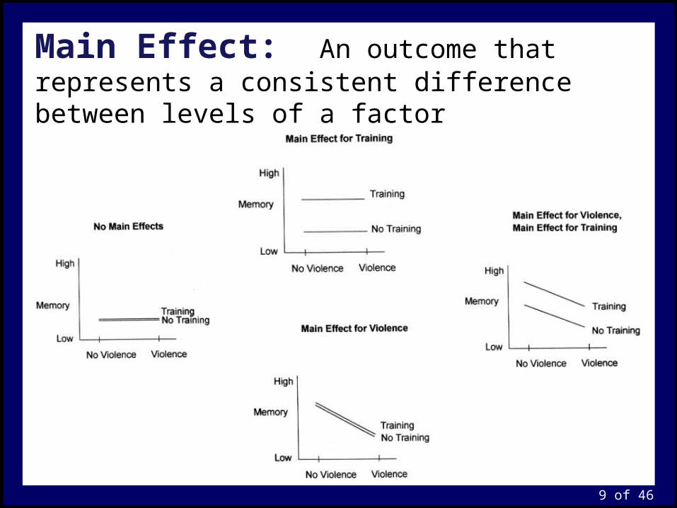
Main Effect: An outcome that represents a consistent difference between levels of a factor

10 of 46

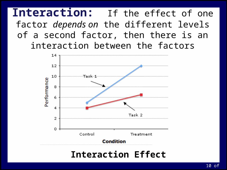
Interaction: If the effect of one factor depends on the different levels of a second factor, then there

is an interaction between the factors

Interaction Effect

11 of 46

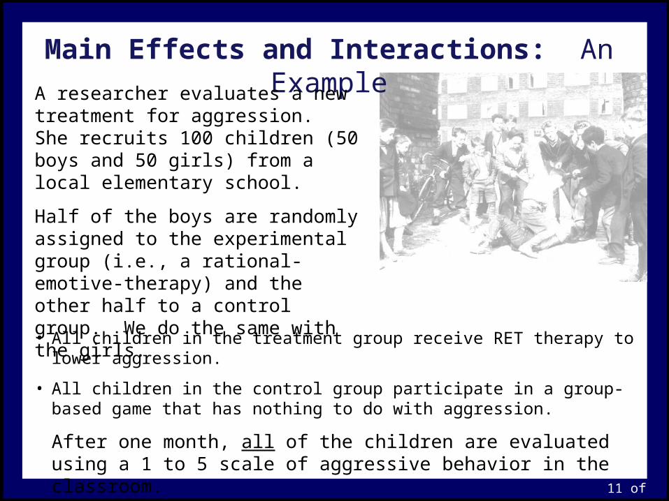
Main Effects and Interactions: An Example

A researcher evaluates a new treatment for aggression. She recruits 100 children (50 boys and 50 girls) from a local elementary school.

Half of the boys are randomly assigned to the experimental group (i.e., a rational-emotive-therapy) and the other half to a control group. We do the same with the girls.

• All children in the treatment group receive RET therapy to lower aggression.

• All children in the control group participate in a group-based game that has nothing to do with aggression.

After one month, all of the children are evaluated using a 1 to 5 scale of aggressive behavior in the classroom.

12 of 46

Main Effects: When there are differences among the levels of a single factor, ignoring the other factor, we say there is a main effect of that factor.

• Ignoring treatment condition, are there gender differences in aggressive behavior? This is the main effect of gender.

• Ignoring gender, is there evidence that the therapy condition decreases aggressive behavior compared to the control condition? This is the main effect of treatment.

Interaction EffectsDo boys and girls respond differently to the same therapy? This is the interaction between gender and treatment.

In our study of children’s aggression, the presence of an interaction suggests the therapy affects boys and girls differently. “It depends” is another way of describing an interaction: the effect of factor 1 depends on the level of factor 2.

13 of 46

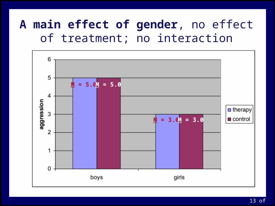
A main effect of gender, no effect of treatment; no interaction

M = 5.0 M = 5.0

M = 3.0 M = 3.0

14 of 46

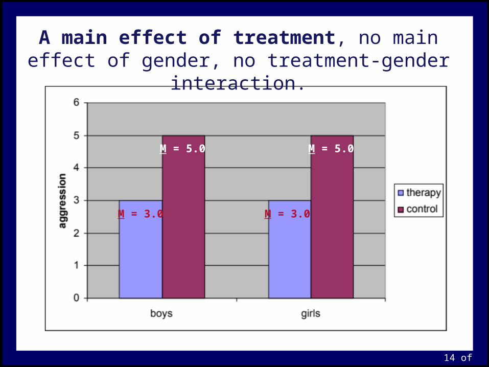
A main effect of treatment, no main effect of gender, no treatment-gender interaction.

M = 3.0

M = 5.0M = 5.0

M = 3.0

15 of 46

A main effect of treatment, a main effect of gender, no treatment-gender interaction

M = 3.0

M = 5.0

M = 2.0

M = 4.0

16 of 46

An interaction between treatment and gender; main effect of treatment; no main effect of gender

M = 5.0

M = 4.0

M = 2.0

M = 3.0

17 of 46

An interaction between treatment and gender; no main effect of treatment or gender

M = 2.0

M = 5.0M = 5.0

M = 2.0

18 of 46

Factorial ANOVA: An Example

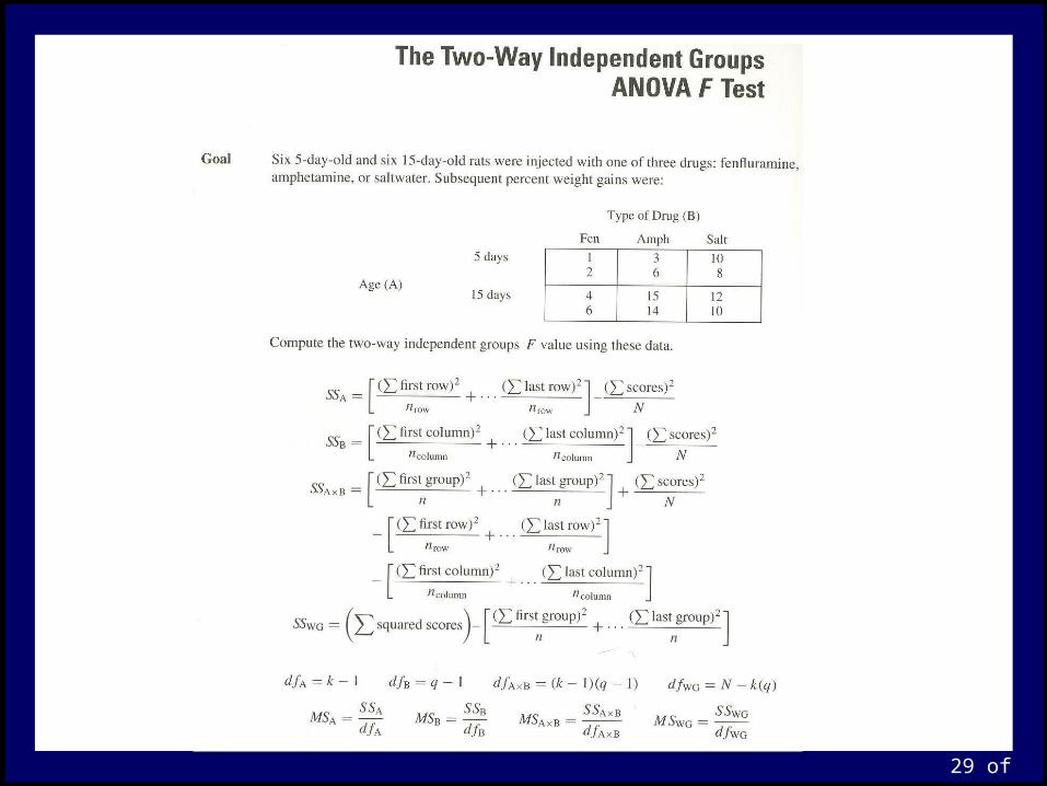
Imagine the following scenario:– A researcher compares the appetite suppressing effects of fenfluramine,

amphetamine, and saltwater injections in 15-day old rats. The results show that fenfluramine produces greater appetite suppression than saltwater, but fenfluramine and amphetamine do not differ.

– The researcher further hypothesizes that the relationship between type of drug and appetite suppression varies depending on whether the rats are 5 or 15-days-old.

This suggests the existence of a moderator effect: a relationship involving three variables in which the relationship between two of the variables differs depending upon the third variable.

If the relationship between drug and percent weight gain varies depending on the age of the rats, then age moderates the relationship between type of drug and weight gain.

19 of 46

Defining the Null & Alternative HypothesesThe Age Main Effect: The omnibus test evaluates whether the percent

weight gain is different for 5-day-old rats than for 15-day-old rats

H0: µ5 = µ15

H1: µ5 = µ15

The Drug Main Effect: The omnibus test evaluates whether there are differences in percentage weight gain depending on whether the rat is injected with fenfluramine, amphetamine, or saltwater in a population of 5 and15-day-old rats

H0: µF = µA = µS

H1: not all µs are equal

The Age-Drug Interaction: If the proposed moderator effect exists, the relationship between type of drug and percent weight gain should be different depending on age, and the relationship between age and percent weight gain should be different depending on the type of drug.

H0: (µ5F - µ15F) = (µ5A - µ15A)) = (µ5S - µ15S))

H1: differences between µs at different ages vary depending on type of drug

20 of 46

Graphical Depiction of Main Effect of Age

Mean percent weight gain is different for 5-day-old rats than for 15-day-old rats

Mean = 13

Mean = 11

21 of 46

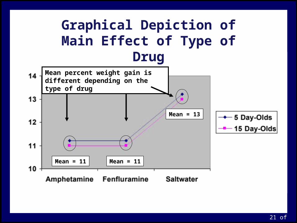
Graphical Depiction of Main Effect of Type of Drug

Mean percent weight gain is different depending on the type of drug

Mean = 11 Mean = 11

Mean = 13

22 of 46

Graphical Depiction of an Interaction between Age and Type of Drug, but no Main Effects

Type of Drug

Fenfluramine Amphetamine Saltwater

Age 5 day-old 15 13 11 13

15 day-old 11 13 15 13

13 13 13 13

23 of 46

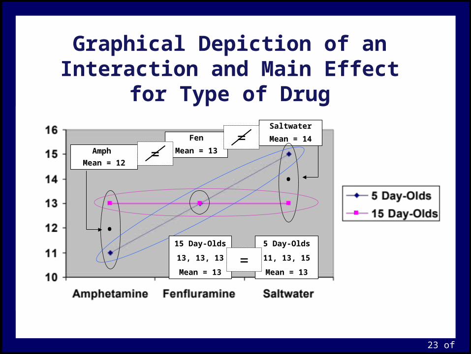
Graphical Depiction of an Interaction and Main Effect for Type of Drug

Amph

Mean = 12

Fen

Mean = 13

Saltwater

Mean = 14

•

•

15 Day-Olds

13, 13, 13

Mean = 13

5 Day-Olds

11, 13, 15

Mean = 13=

==

24 of 46

-- Three F tests required: one for each factor (Factor A; Factor B), and a third for the interaction (A x B).

-- The numerator differs for the three F tests, but the denominator for all three is the MSWG.

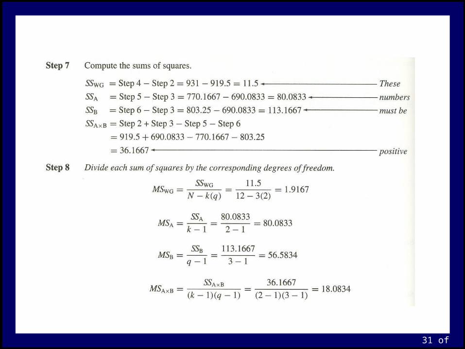
-- Calculate the sum of squares for factor A (SSA), factor B (SSB), the interaction (SSAxB), and the error term (SSWG).

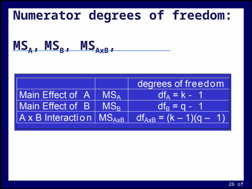
-- Convert each factor’s SS to the average sums of square or “mean squares” (MS) by dividing by the appropriate degrees of freedom).

Two-way Independent-groups ANOVA: Steps in the Analysis

FA = MSA FB = MSB FAxB = MSAxB

MSWG MSWG MSWG

25 of 46

SSWG = ( squared scores) – ( first group)2 + ( last group)2

n n Denominator degrees of freedom: dfWG = N – k(q)

Computing the Denominator: MSWG

Note: k = number of groups in Factor A q = number of groups in Factor B

MSWG =SSWG

dfWG

26 of 46

Numerator degrees of freedom: MSA, MSB, MSAxB,

27 of 46

Computing a Two-way Independent-groups

ANOVA by hand

28 of 46

1 Fen 5 Day 12 Fen 5 Day 23 Fen 15 Day 44 Fen 15 Day 65 Amph 5 Day 36 Amph 5 Day 67 Amph 15 Day 158 Amph 15 Day 149 Salt 5 Day 1010 Salt 5 Day 811 Salt 15 Day 1212 Salt 15 Day 10

Data SetSubject Type of Age Percent Drug Weight Gain

29 of 46

30 of 46

31 of 46

32 of 46

33 of 46

Critical Values for F

34 of 46

Computing the Two-way Independent-groups ANOVA using SPSS

35 of 46

SPSS Data Editor

36 of 46

37 of 46

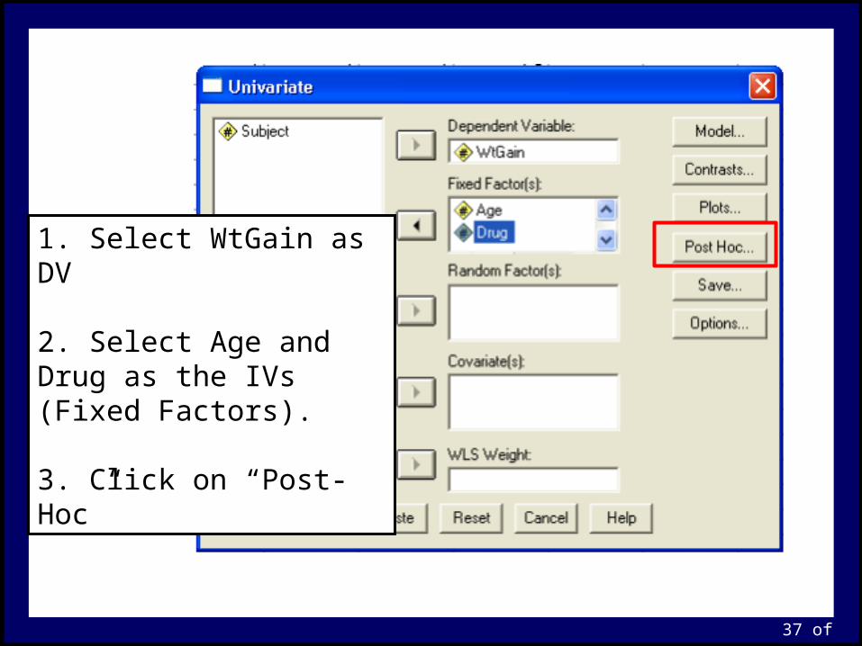
1. Select WtGain as DV

2. Select Age and Drug as the IVs (Fixed Factors).

3. Click on “Post-Hoc”

38 of 46

Now … think carefully!

Which of the IVs requires a follow-up (post-hoc) test?

Which post-hoc procedure(s) will you choose? Why?

39 of 46

Note that you can also get follow-up tests by clicking on the “Options” button. This box also allows you to get “Descriptive Statistics”, “Estimates of Effect Size”, and “Homogeneity Tests”, if you want these …

40 of 46

Descriptive Statistics

41 of 46

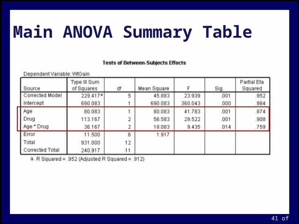
Main ANOVA Summary Table

42 of 46

Post-hoc Tests: Age

Did we need to request a post-hoc test for the “Age” factor?

Why or why not?

43 of 46

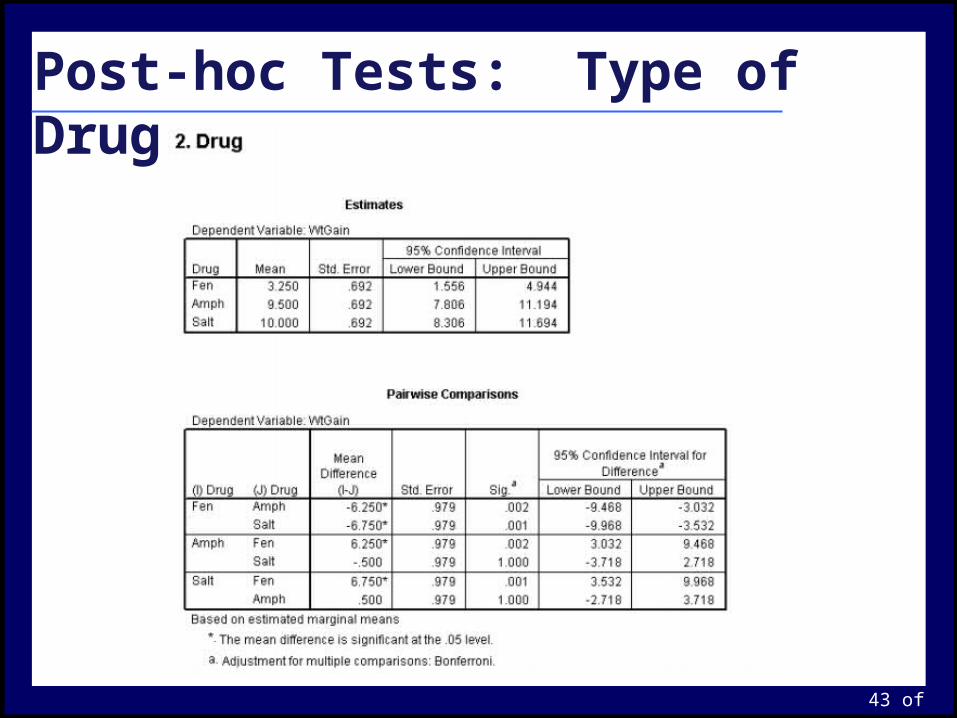
Post-hoc Tests: Type of Drug

44 of 46

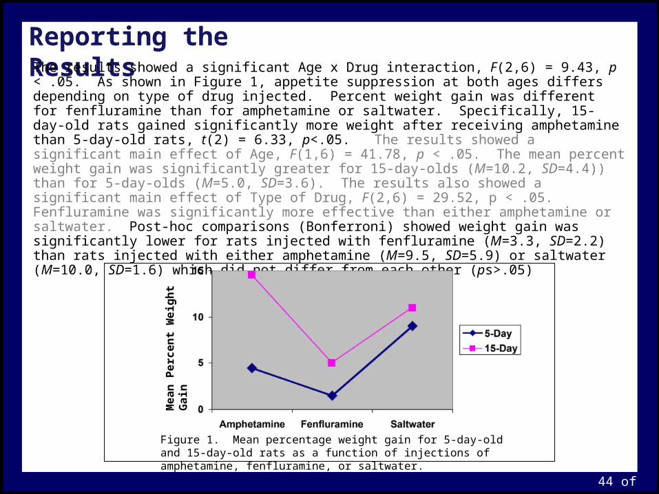
Reporting the ResultsThe results showed a significant Age x Drug interaction, F(2,6) = 9.43, p < .05. As shown in Figure 1, appetite suppression at both ages differs depending on type of drug injected. Percent weight gain was different for fenfluramine than for amphetamine or saltwater. Specifically, 15-day-old rats gained significantly more weight after receiving amphetamine than 5-day-old rats, t(2) = 6.33, p<.05. The results showed a significant main effect of Age, F(1,6) = 41.78, p < .05. The mean percent weight gain was significantly greater for 15-day-olds (M=10.2, SD=4.4)) than for 5-day-olds (M=5.0, SD=3.6). The results also showed a significant main effect of Type of Drug, F(2,6) = 29.52, p < .05. Fenfluramine was significantly more effective than either amphetamine or saltwater. Post-hoc comparisons (Bonferroni) showed weight gain was significantly lower for rats injected with fenfluramine (M=3.3, SD=2.2) than rats injected with either amphetamine (M=9.5, SD=5.9) or saltwater (M=10.0, SD=1.6) which did not differ from each other (ps>.05)

Me

an

Pe

rce

nt

We

igh

t G

ain

Figure 1. Mean percentage weight gain for 5-day-old and 15-day-old rats as a function of injections of amphetamine, fenfluramine, or saltwater.

45 of 46

2effect =

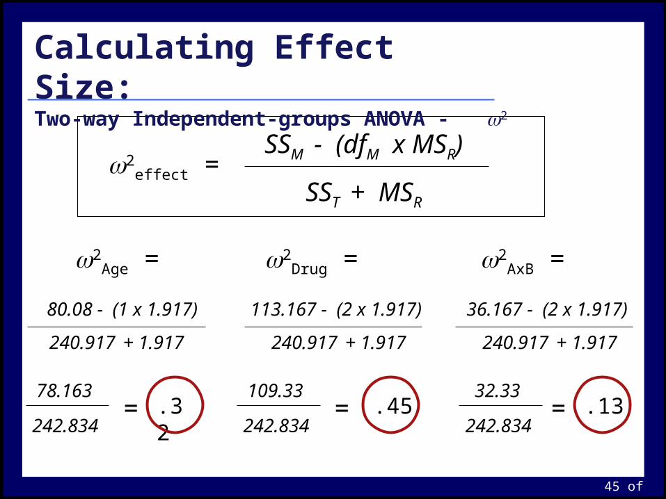
Calculating Effect Size: Two-way Independent-groups ANOVA - 2

SSM - (dfM x MSR)

SST + MSR

80.08 - (1 x 1.917)

240.917 + 1.917

2Age =

78.163

242.834

= .32

113.167 - (2 x 1.917)

2Drug =

109.33

242.834

= .45

240.917 + 1.917

36.167 - (2 x 1.917)

2AxB =

32.33

242.834

= .13

240.917 + 1.917

46 of 46

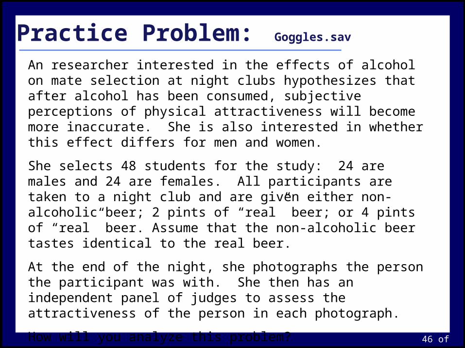
Practice Problem: Goggles.sav

An researcher interested in the effects of alcohol on mate selection at night clubs hypothesizes that after alcohol has been consumed, subjective perceptions of physical attractiveness will become more inaccurate. She is also interested in whether this effect differs for men and women.

She selects 48 students for the study: 24 are males and 24 are females. All participants are taken to a night club and are given either non-alcoholic beer; 2 pints of “real” beer; or 4 pints of “real” beer. Assume that the non-alcoholic beer tastes identical to the real beer.

At the end of the night, she photographs the person the participant was with. She then has an independent panel of judges to assess the attractiveness of the person in each photograph.

How will you analyze this problem?