1 of 19 Digital Image Processing Image Enhancement- Spatial Filtering From: Digital Image...

1of19

Digital Image Processing

Image Enhancement- Spatial Filtering

From:

Digital Image Processing, Chapter 3

Refael C. Gonzalez & Richard E. Woods

2of19

Contents

Next, we will look at spatial filtering techniques:

– What is spatial filtering?– Smoothing Spatial filters.– Sharpening Spatial Filters.– Combining Spatial Enhancement Methods

3of19

Neighbourhood Operations

Neighbourhood operations simply operate on a larger neighbourhood of pixels than point operations

Neighbourhoods are mostly a rectangle around a central pixel

Any size rectangle and any shape filter are possible

Origin x

y Image f (x, y)

(x, y)Neighbourhood

4of19

Neighbourhood Operations

For each pixel in the origin image, the outcome is written on the same location at the target image.

Origin x

y Image f (x, y)

(x, y)Neighbourhood

TargetOrigin

5of19

Simple Neighbourhood Operations

Simple neighbourhood operations example:

– Min: Set the pixel value to the minimum in the neighbourhood

– Max: Set the pixel value to the maximum in the neighbourhood

6of19

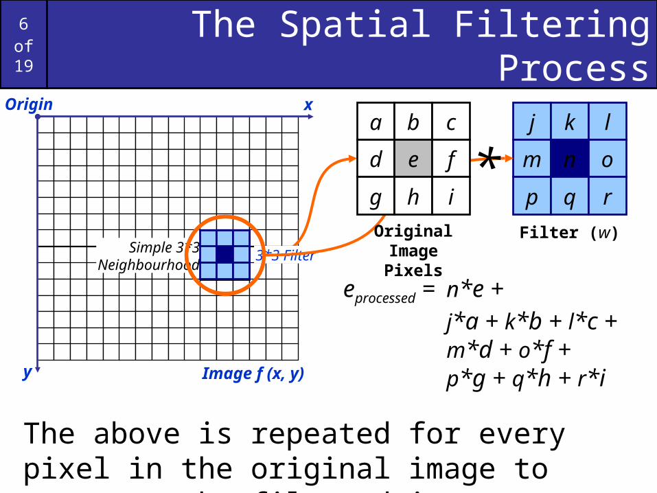
The Spatial Filtering Process

j k l

m n o

p q r

Origin x

y Image f (x, y)

eprocessed = n*e + j*a + k*b + l*c + m*d + o*f + p*g + q*h + r*i

Filter (w)Simple 3*3

Neighbourhoode 3*3 Filter

a b c

d e f

g h i

Original Image Pixels

*

The above is repeated for every pixel in the original image to generate the filtered image

7of19

Spatial Filtering: Equation Form

a

as

b

bt

tysxftswyxg ),(),(),(

Filtering can be given in equation form as shown above

Notations are based on the image shown to the left

Ima

ge

s ta

ken

fro

m G

on

zale

z &

Wo

od

s, D

igita

l Im

ag

e P

roce

ssin

g (

20

02

)

8of19

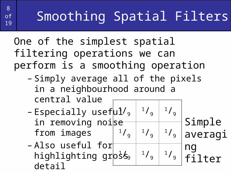
Smoothing Spatial Filters

One of the simplest spatial filtering operations we can perform is a smoothing operation

– Simply average all of the pixels in a neighbourhood around a central value

– Especially useful in removing noise from images

– Also useful for highlighting gross detail

1/91/9

1/9

1/91/9

1/9

1/91/9

1/9

Simple averaging filter

9of19

Smoothing Spatial Filtering

1/91/9

1/9

1/91/9

1/9

1/91/9

1/9

Origin x

y Image f (x, y)

e = 1/9*106 + 1/9*104 + 1/9*100 + 1/9*108 + 1/9*99 + 1/9*98 + 1/9*95 + 1/9*90 + 1/9*85

= 98.3333

FilterSimple 3*3

Neighbourhood106

104

99

95

100 108

98

90 85

1/91/9

1/9

1/91/9

1/9

1/91/9

1/9

3*3 SmoothingFilter

104 100 108

99 106 98

95 90 85


*

The above is repeated for every pixel in the original image to generate the smoothed image

10of19

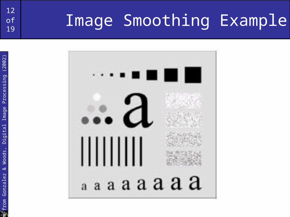
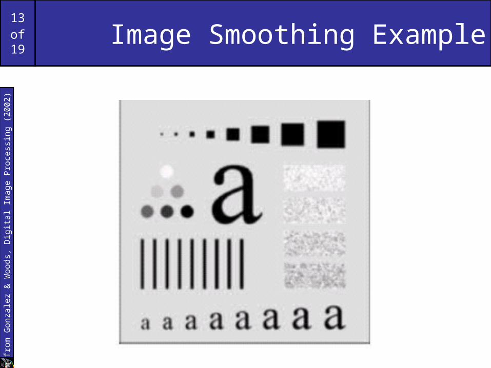
Image Smoothing Example

The image at the top left is an original image of size 500*500 pixels

The subsequent images show the image after filtering with an averaging filter of increasing sizes

– 3, 5, 9, 15 and 35

Notice how detail begins to disappear

Ima

ge

s ta

ken

fro

m G

on

zale

z &

Wo

od

s, D

igita

l Im

ag

e P

roce

ssin

g (

20

02

)

11of19

Image Smoothing ExampleIm

ag

es

take

n f

rom

Go

nza

lez

& W

oo

ds,

Dig

ital I

ma

ge

Pro

cess

ing

(2

00

2)

12of19


ag

es

take

n f

rom

Go

nza

lez

& W

oo

ds,

Dig

ital I

ma

ge

Pro

cess

ing

(2

00

2)

13of19


ag

es

take

n f

rom

Go

nza

lez

& W

oo

ds,

Dig

ital I

ma

ge

Pro

cess

ing

(2

00

2)

14of19


ag

es

take

n f

rom

Go

nza

lez

& W

oo

ds,

Dig

ital I

ma

ge

Pro

cess

ing

(2

00

2)

15of19


ag

es

take

n f

rom

Go

nza

lez

& W

oo

ds,

Dig

ital I

ma

ge

Pro

cess

ing

(2

00

2)

16of19


ag

es

take

n f

rom

Go

nza

lez

& W

oo

ds,

Dig

ital I

ma

ge

Pro

cess

ing

(2

00

2)

17of19

Weighted Smoothing Filters

More effective smoothing filters can be generated by allowing different pixels in the neighbourhood different weights in the averaging function

– Pixels closer to the central pixel are more important

– Often referred to as a weighted averaging

1/162/16

1/16

2/164/16

2/16

1/162/16

1/16

Weighted averaging filter

18of19

Another Smoothing Example

By smoothing the original image we get rid of lots of the finer detail which leaves only the gross features for thresholding

Ima

ge

s ta

ken

fro

m G

on

zale

z &

Wo

od

s, D

igita

l Im

ag

e P

roce

ssin

g (

20

02

)

Original Image Smoothed Image Thresholded Image

* Image taken from Hubble Space Telescope

19of19

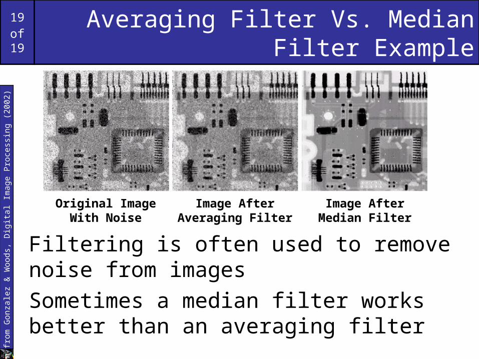
Averaging Filter Vs. Median Filter Example

Filtering is often used to remove noise from images

Sometimes a median filter works better than an averaging filter

Original ImageWith Noise

Image AfterAveraging Filter

Image AfterMedian Filter

Ima

ge

s ta

ken

fro

m G

on

zale

z &

Wo

od

s, D

igita

l Im

ag

e P

roce

ssin

g (

20

02

)

20of19


Ima

ge

s ta

ken

fro

m G

on

zale

z &

Wo

od

s, D

igita

l Im

ag

e P

roce

ssin

g (

20

02

)

Original

21of19


Ima

ge

s ta

ken

fro

m G

on

zale

z &

Wo

od

s, D

igita

l Im

ag

e P

roce

ssin

g (

20

02

)

AveragingFilter

22of19


Ima

ge

s ta

ken

fro

m G

on

zale

z &

Wo

od

s, D

igita

l Im

ag

e P

roce

ssin

g (

20

02

)

MedianFilter

23of19

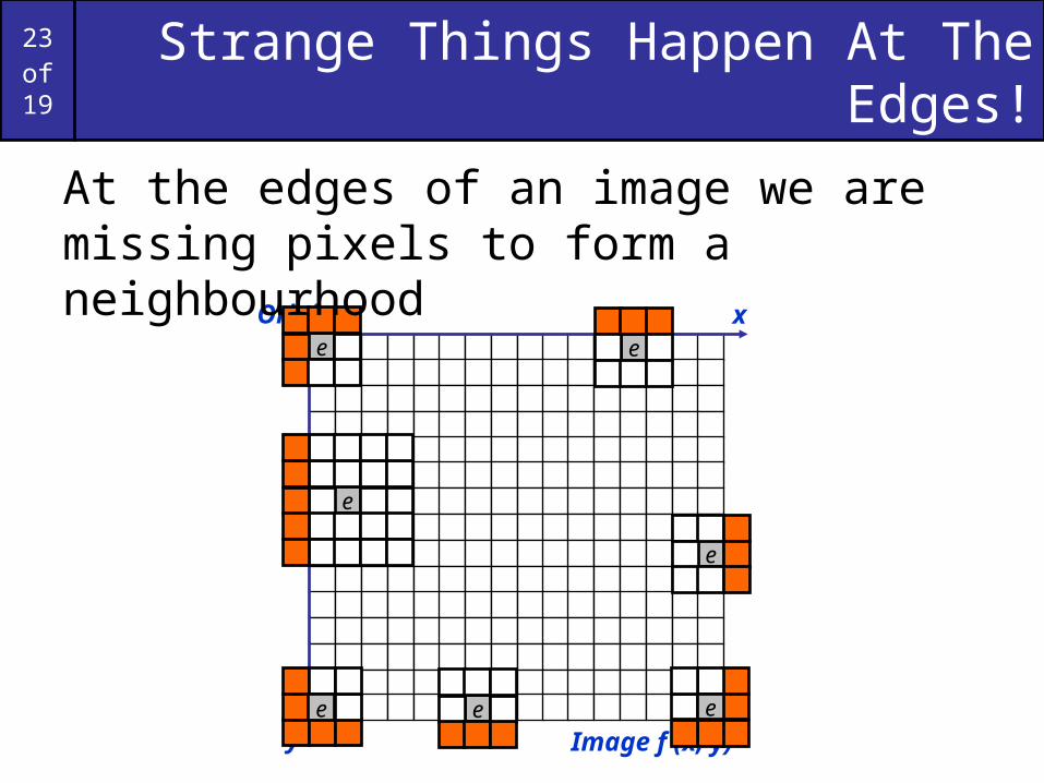
Strange Things Happen At The Edges!

Origin x

y Image f (x, y)

e

e

e

e

At the edges of an image we are missing pixels to form a neighbourhood

e e

e

24of19

Strange Things Happen At The Edges! (cont…)

There are a few approaches to dealing with missing edge pixels:

– Omit missing pixels• Only works with some filters• Can add extra code and slow down processing

– Pad the image • Typically with either all white or all black pixels

– Replicate border pixels– Truncate the image

25of19

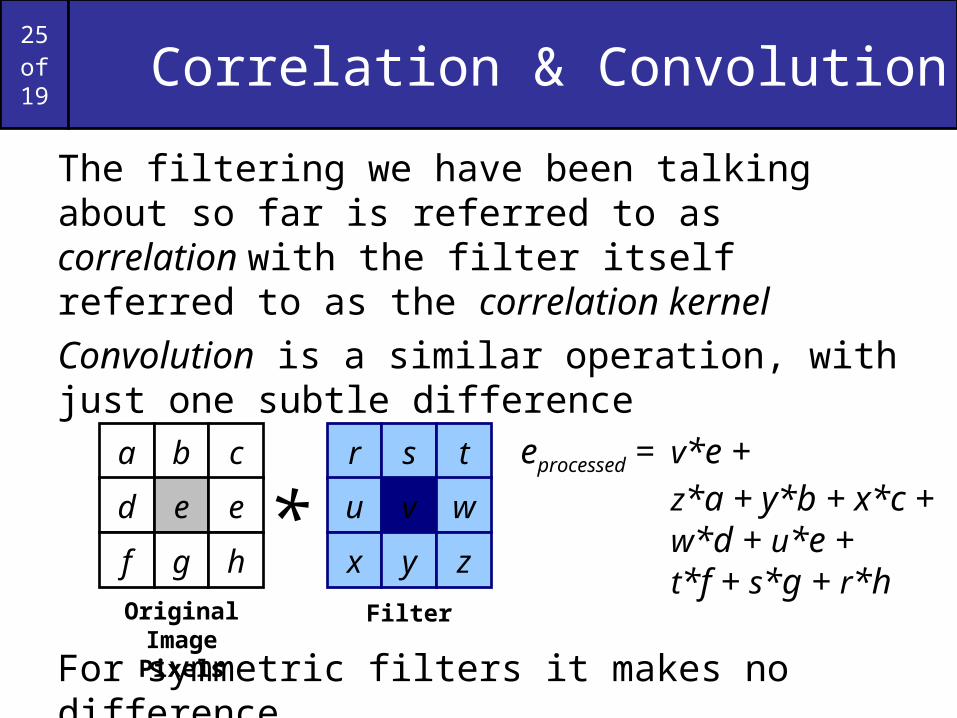
Correlation & Convolution

The filtering we have been talking about so far is referred to as correlation with the filter itself referred to as the correlation kernel

Convolution is a similar operation, with just one subtle difference

For symmetric filters it makes no difference

eprocessed = v*e + z*a + y*b + x*c + w*d + u*e + t*f + s*g + r*h

r s t

u v w

x y z

Filter

a b c

d e e

f g h


*

26of19

Sharpening Spatial Filters

Previously we have looked at smoothing filters which remove fine detail

Sharpening spatial filters seek to highlight fine detail

– Remove blurring from images– Highlight edges

Sharpening filters are based on spatial differentiation

27of19

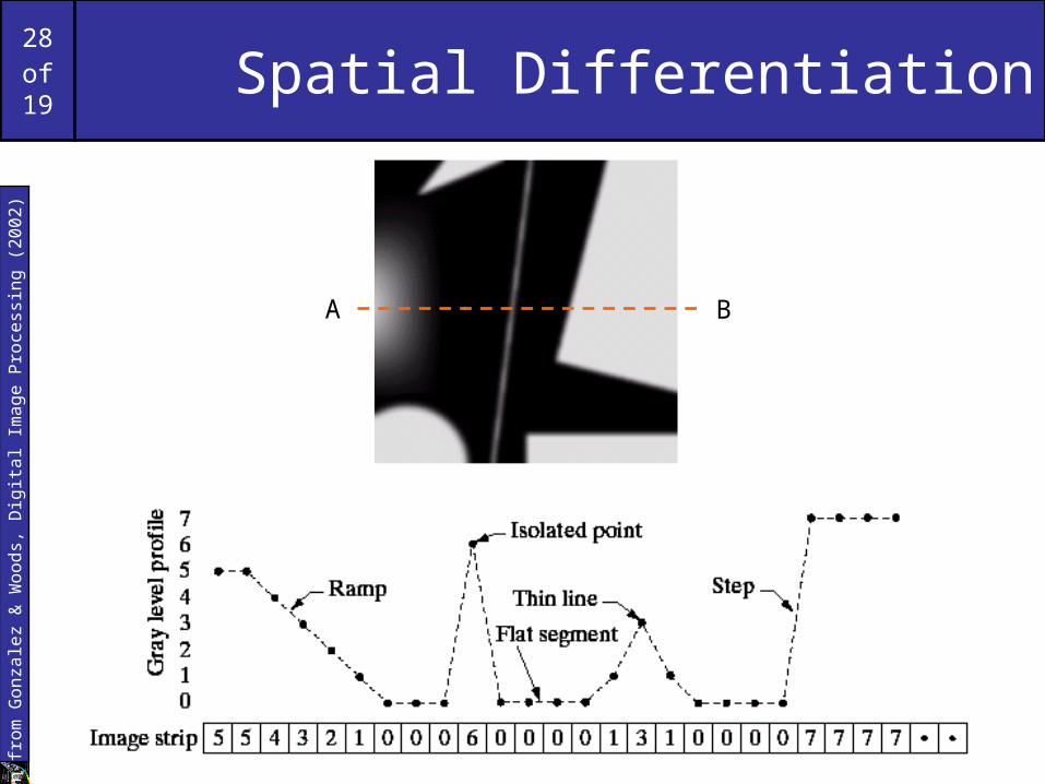
Spatial Differentiation

Differentiation measures the rate of change of a function

Let’s consider a simple 1 dimensional example

Ima

ge

s ta

ken

fro

m G

on

zale

z &

Wo

od

s, D

igita

l Im

ag

e P

roce

ssin

g (

20

02

)

28of19

Spatial DifferentiationIm

ag

es

take

n f

rom

Go

nza

lez

& W

oo

ds,

Dig

ital I

ma

ge

Pro

cess

ing

(2

00

2)

A B

29of19

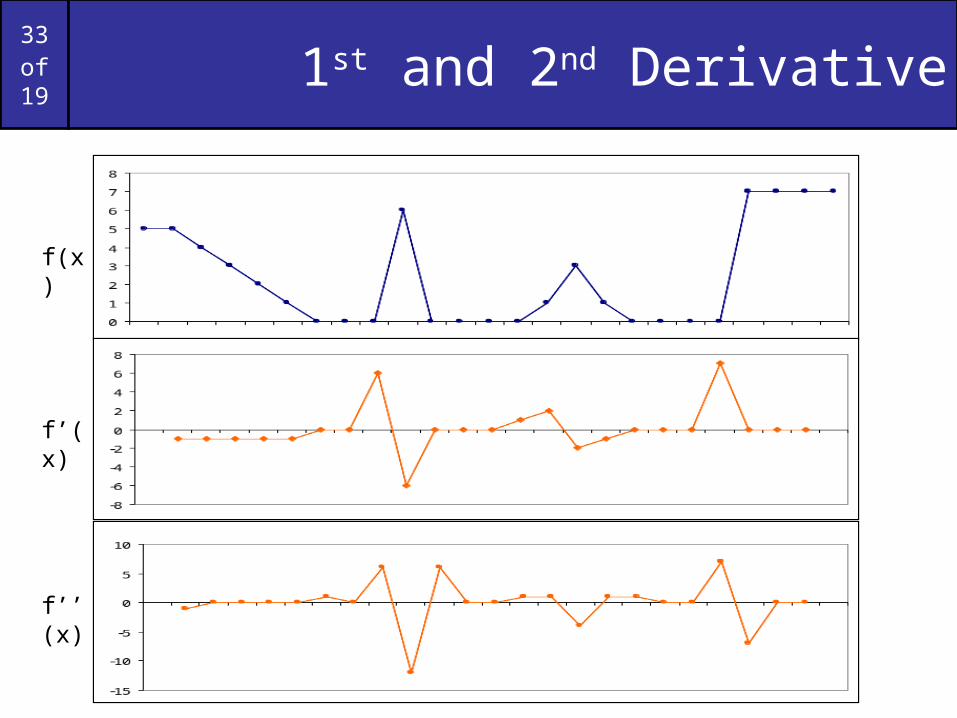
1st Derivative

The formula for the 1st derivative of a function is as follows:

It’s just the difference between subsequent values and measures the rate of change of the function

)()1( xfxfx

f

30of19

1st Derivative (cont…)

5 5 4 3 2 1 0 0 0 6 0 0 0 0 1 3 1 0 0 0 0 7 7 7 7

0 -1 -1 -1 -1 0 0 6 -6 0 0 0 1 2 -2 -1 0 0 0 7 0 0 0

f(x)

f’(x)

31of19

2nd Derivative

The formula for the 2nd derivative of a function is as follows:

Simply takes into account the values both before and after the current value

)(2)1()1(2

2

xfxfxfx

f

32of19

2nd Derivative (cont…)

5 5 4 3 2 1 0 0 0 6 0 0 0 0 1 3 1 0 0 0 0 7 7 7 7

-1 0 0 0 0 1 0 6 -12 6 0 0 1 1 -4 1 1 0 0 7 -7 0 0

f(x)

f’’(x)

33of19

1st and 2nd Derivative

f(x)

f’(x)

f’’(x)

34of19

Using Second Derivatives For Image Enhancement

The 2nd derivative is more useful for image enhancement than the 1st derivative

– Stronger response to fine detail– Simpler implementation– We will come back to the 1st order derivative

later on

The first sharpening filter we will look at is the Laplacian

– Isotropic– One of the simplest sharpening filters– We will look at a digital implementation

35of19

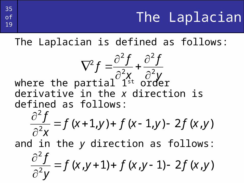
The Laplacian

The Laplacian is defined as follows:

where the partial 1st order derivative in the x direction is defined as follows:

and in the y direction as follows:

y

f

x

ff

2

2

2

22

),(2),1(),1(2

2

yxfyxfyxfx

f

),(2)1,()1,(2

2

yxfyxfyxfy

f

36of19

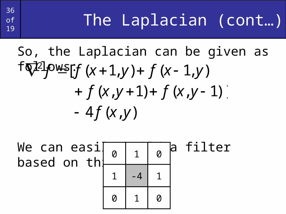
The Laplacian (cont…)

So, the Laplacian can be given as follows:

We can easily build a filter based on this

),1(),1([2 yxfyxff )]1,()1,( yxfyxf

),(4 yxf

0 1 0

1 -4 1

0 1 0

37of19

The Laplacian (cont…)

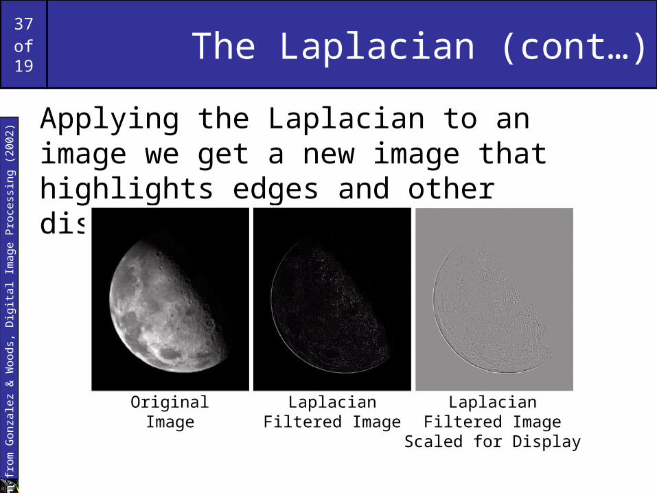
Applying the Laplacian to an image we get a new image that highlights edges and other discontinuities

Ima

ge

s ta

ken

fro

m G

on

zale

z &

Wo

od

s, D

igita

l Im

ag

e P

roce

ssin

g (

20

02

)

OriginalImage

LaplacianFiltered Image


Scaled for Display

38of19

But That Is Not Very Enhanced!

The result of a Laplacian filtering is not an enhanced image

We have to do more work in order to get our final image

Subtract the Laplacian result from the original image to generate our final sharpened enhanced image


Scaled for Display

Ima

ge

s ta

ken

fro

m G

on

zale

z &

Wo

od

s, D

igita

l Im

ag

e P

roce

ssin

g (

20

02

)

fyxfyxg 2),(),(

39of19

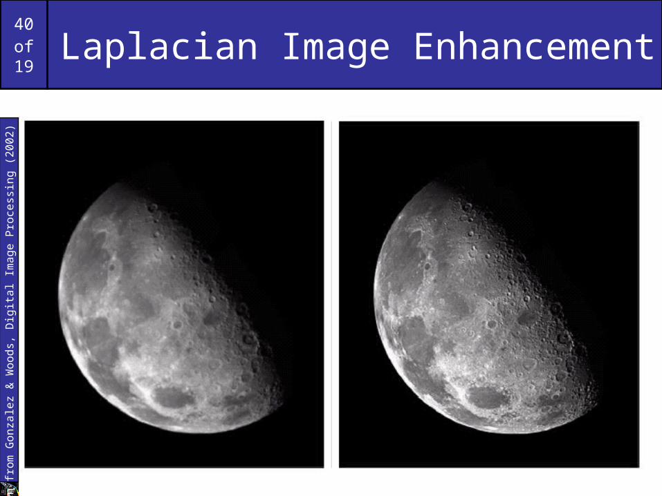
Laplacian Image Enhancement

In the final sharpened image edges and fine detail are much more obvious

Ima

ge

s ta

ken

fro

m G

on

zale

z &

Wo

od

s, D

igita

l Im

ag

e P

roce

ssin

g (

20

02

)

- =

OriginalImage


SharpenedImage

40of19

Laplacian Image EnhancementIm

ag

es

take

n f

rom

Go

nza

lez

& W

oo

ds,

Dig

ital I

ma

ge

Pro

cess

ing

(2

00

2)

41of19

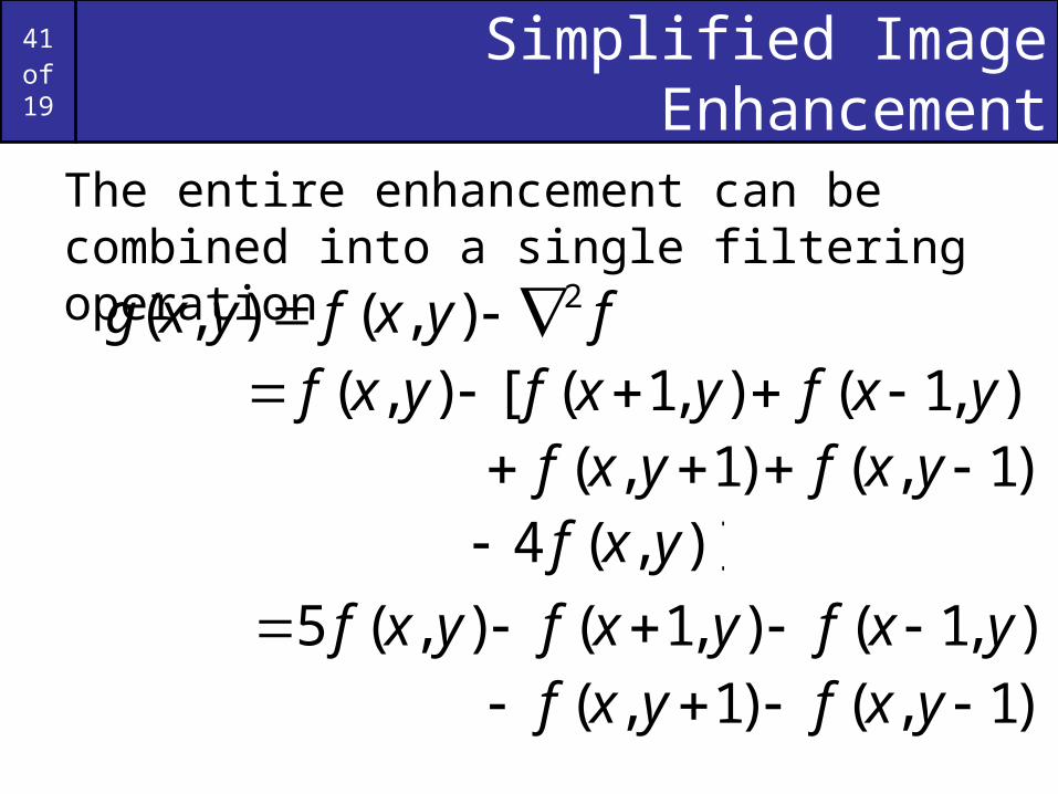
Simplified Image Enhancement

The entire enhancement can be combined into a single filtering operation

),1(),1([),( yxfyxfyxf )1,()1,( yxfyxf

)],(4 yxf

fyxfyxg 2),(),(

),1(),1(),(5 yxfyxfyxf )1,()1,( yxfyxf

42of19

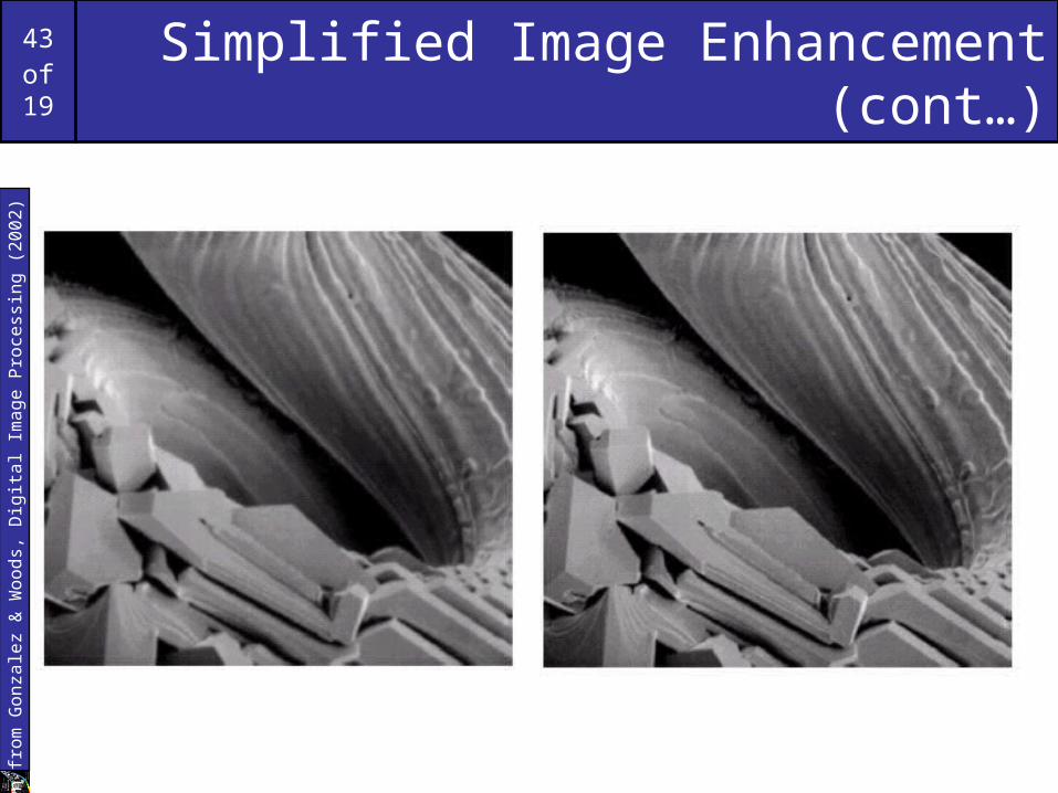
Simplified Image Enhancement (cont…)

This gives us a new filter which does the whole job for us in one step

0 -1 0

-1 5 -1

0 -1 0

Ima

ge

s ta

ken

fro

m G

on

zale

z &

Wo

od

s, D

igita

l Im

ag

e P

roce

ssin

g (

20

02

)

43of19

Simplified Image Enhancement (cont…)Im

ag

es

take

n f

rom

Go

nza

lez

& W

oo

ds,

Dig

ital I

ma

ge

Pro

cess

ing

(2

00

2)

44of19

Variants On The Simple Laplacian

There are lots of slightly different versions of the Laplacian that can be used:

0 1 0

1 -4 1

0 1 0

1 1 1

1 -8 1

1 1 1

-1 -1 -1

-1 9 -1

-1 -1 -1

SimpleLaplacian

Variant ofLaplacian

Ima

ge

s ta

ken

fro

m G

on

zale

z &

Wo

od

s, D

igita

l Im

ag

e P

roce

ssin

g (

20

02

)

45of19

Unsharp Mask & Highboost Filtering

Using sequence of linear spatial filters in order to get Sharpening effect.

-Blur

- Subtract from original image

- add resulting mask to original image

46of19

Highboost Filtering

47of19

1st Derivative Filtering

Implementing 1st derivative filters is difficult in practice

For a function f(x, y) the gradient of f at coordinates (x, y) is given as the column vector:

y

fx

f

G

G

y

xf

48of19

1st Derivative Filtering (cont…)

The magnitude of this vector is given by:

For practical reasons this can be simplified as:

)f( magf

21

22yx GG

21

22

y

f

x

f

yx GGf

49of19

1st Derivative Filtering (cont…)

There is some debate as to how best to calculate these gradients but we will use:

which is based on these coordinates

321987 22 zzzzzzf

741963 22 zzzzzz

z1 z2 z3

z4 z5 z6

z7 z8 z9

50of19

Sobel Operators

Based on the previous equations we can derive the Sobel Operators

To filter an image it is filtered using both operators the results of which are added together

-1 -2 -1

0 0 0

1 2 1

-1 0 1

-2 0 2

-1 0 1

51of19

Sobel Example

Sobel filters are typically used for edge detection

Ima

ge

s ta

ken

fro

m G

on

zale

z &

Wo

od

s, D

igita

l Im

ag

e P

roce

ssin

g (

20

02

)

An image of a contact lens which is enhanced in order to make defects (at four and five o’clock in the image) more obvious

52of19

1st & 2nd Derivatives

Comparing the 1st and 2nd derivatives we can conclude the following:

– 1st order derivatives generally produce thicker edges

– 2nd order derivatives have a stronger response to fine detail e.g. thin lines

– 1st order derivatives have stronger response to grey level step

– 2nd order derivatives produce a double response at step changes in grey level

53of19

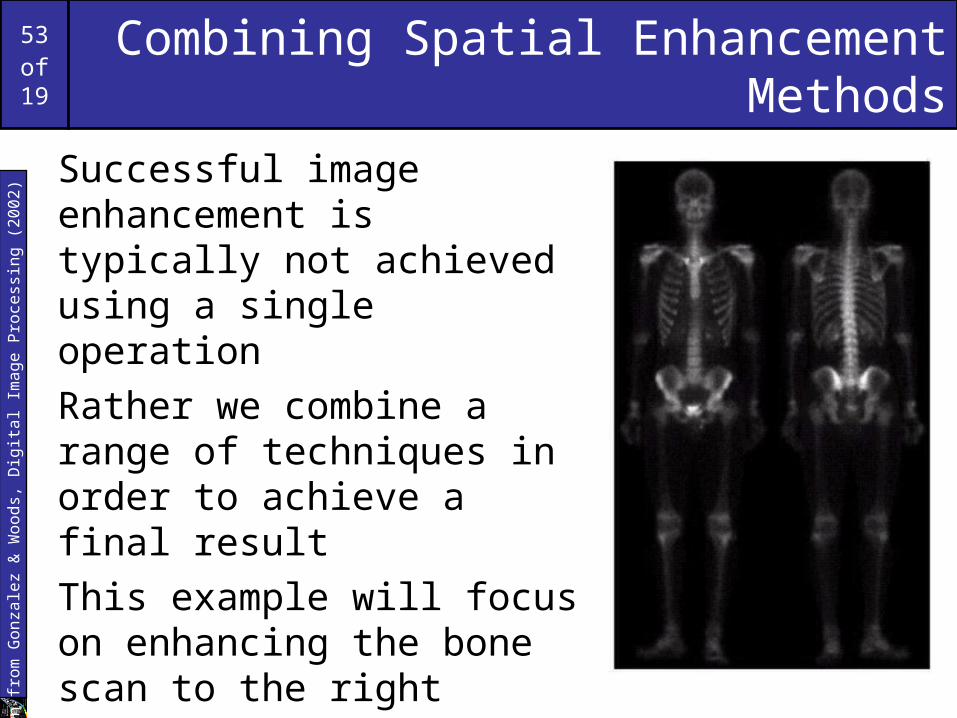
Combining Spatial Enhancement Methods

Successful image enhancement is typically not achieved using a single operation

Rather we combine a range of techniques in order to achieve a final result

This example will focus on enhancing the bone scan to the right

Ima

ge

s ta

ken

fro

m G

on

zale

z &

Wo

od

s, D

igita

l Im

ag

e P

roce

ssin

g (

20

02

)

54of19

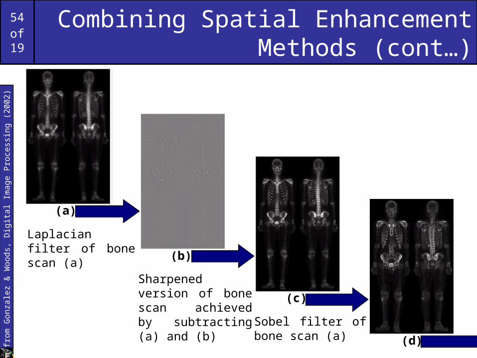
Combining Spatial Enhancement Methods (cont…)

Ima

ge

s ta

ken

fro

m G

on

zale

z &

Wo

od

s, D

igita

l Im

ag

e P

roce

ssin

g (

20

02

)

Laplacian filter of bone scan (a)

Sharpened version of bone scan achieved by subtracting (a) and (b) Sobel filter of bone

scan (a)

(a)

(b)

(c)

(d)

55of19


Ima

ge

s ta

ken

fro

m G

on

zale

z &

Wo

od

s, D

igita

l Im

ag

e P

roce

ssin

g (

20

02

)

The product of (c) and (e) which will be used as a mask

Sharpened image which is sum of (a) and (f)

Result of applying a power-law trans. to (g)

(e)

(f)

(g)

(h)

Image (d) smoothed with a 5*5 averaging filter

56of19


Compare the original and final images

Ima

ge

s ta

ken

fro

m G

on

zale

z &

Wo

od

s, D

igita

l Im

ag

e P

roce

ssin

g (

20

02

)

1 of 19 Digital Image Processing Image Enhancement- Spatial Filtering From: Digital Image...

Documents

Transcript of 1 of 19 Digital Image Processing Image Enhancement- Spatial Filtering From: Digital Image...