1 Notes for Methods IB by C. P. Caul eld - University of...

1

Notes for

Methods IB

by C. P. Caulfield

c© C.P. Caulfield (2007, 2008, 2009). All rights reserved. 27/12/09

2

These notes cover the Methods IB course as taught by me, (Dr ColmCaulfield) in Michaelmas 2009. They have grown out of the course as taughtby Professor Nigel Peake to whom heartfelt thanks are offered for access tohis notes, but have been modified substantially in both content and ordering.Naturally, I am responsible for any errors, and would be very glad to be toldabout any such errors by email to [email protected]. This copyincludes the corrections to a startlingly large number of typos that appearedduring the lecturing in previous years. I hope these notes prove a usefuladjunct to attendance at the lectures, and convey some of the extent to whichthis course is really rather groovy. They are not intended as a substitute fora good textbook. . .

Part I

Self-adjoint ODEs

3

Chapter 1

Fourier series

1.1 Periodic functions

A function f(t) is said to be periodic if f(t + T ) = f(t). T is the period.A classic example is the simple harmonic motion of a pendulum oscillatingthrough a small angle. Consider also the sine function:

y(t) = A sinωt.

The necessary jargon (i.e. Maths Your Supervisor Assumes You Know, orMYSAYK for short) is:

• A is the amplitude;

• ω is the frequency;

• T = 2πω

is the period.

Remember, a function can be periodic without being continuous, and lots ofinteresting mathematics occurs for functions which are discontinuous at T ,2T , 3T etc.

Particularly beautiful and useful (because of their orthogonality) classesof periodic functions are sines and cosines. Consider the sets of functionscos(nπxL

)and sin

(nπxL

), (where n is a non-negative integer) which are periodic

∀n on [0, 2L]. Indeed, each component is periodic with period 2L/n forN > 0. Physically, if x is as expected a spatial dimension, 2L/n is thewavelength of the particular trigonometric function. The important bits of

5

6 CHAPTER 1. FOURIER SERIES

MYSAYK here are that:

cos(A±B) = cosA cosB ∓ sinA sinB, and so

cosA cosB =1

2[cos(A−B) + cos(A+B)];

sinA sinB =1

2[cos(A−B)− cos(A+B)].

These expressions are useful when considering the integral SSmn, defined as

SSmn ≡∫ 2L

0

sin(mπx

L

)sin(nπxL

)dx,

=1

2

∫ 2L

0

cos

([m− n]πx

L

)dx− 1

2

∫ 2L

0

cos

([m+ n]πx

L

)dx.

Now if m 6= n,

SSmn =L

2π

sin[

(m−n)πxL

]m− n

−sin[

(m+n)πxL

]m+ n

2L

0

= 0,

while if m = n,

SSmm = L if m 6= 0 or = 0 if m = 0,

where there is no summation convention on m.Therefore, using the Kronecker delta (more MYSAYK, Kronecker being a

German mathematician of the early 19th Century: this course is lousy withGMOTENCs),

SSmn =

{Lδmn ∀m,n 6= 0;

0 m or n = 0.(1.1)

Similarly,

CCmn ≡∫ 2L

0

cos(mπx

L

)cos(nπxL

)dx =

{Lδmn ∀m,n 6= 0;2L n = m = 0.

(1.2)

Finally,

CSmn ≡∫ 2L

0

cos(mπx

L

)sin(nπxL

)dx,

=1

2

∫ 2L

0

sin

([m+ n]πx

L

)dx+

1

2

∫ 2L

0

sin

([n−m]πx

L

)dx,

= 0 ∀m, n. (1.3)

1.2. DEFINITION OF A FOURIER SERIES 7

By analogy with vectors (these integrals are inner products), sin(nπxL

)and

cos(nπxL

)are said to be orthogonal on the interval [0, 2L]. Although it is

not proven here, these functions actually constitute an orthogonal basis forthe space of all functions (with period 2L) and so it is possible to representan arbitrary function as an (infinite) sum of sines and cosines: such a seriesis called a Fourier series after a French mathematician of the early 19thCentury (get used to the FMOTENCs, there’s even more of them about. . . ).

1.2 Definition of a Fourier series

We can express any ‘well-behaved’ periodic function f(x) with period 2L asa Fourier series:

f(x+) + f(x−)

2=

1

2a0 +

∞∑n=1

[an cos

(nπxL

)+ bn sin

(nπxL

)], (1.4)

where an and bn are constants known as the Fourier coefficients, andf(x+) and f(x−) are the right limit approaching from above, and the leftlimit approaching from below respectively.

If f(x) is continuous at the point xc, then the left hand side is of coursejust f(x). However, if f(x) has a bounded discontinuity at the point xd(i.e. the left limit approaching from below f(xd−) 6= f(xd+), the right limitapproaching from above, but |f(xd+)−f(xd−)| is bounded) then the left handside is (precisely) equal to the average of these two limits. It takes a bit ofgetting used to, but is a perfectly reasonable way to define the value of afunction at a bounded discontinuity. Often, this subtlety will be skated over,and the left hand side will just be written as f(x), with the behaviour at abounded discontinuity being understood. Also, the fact that ‘any’ functioncan be described with a Fourier series relies on the fact that sines and cosinesare ‘complete’, a property you may encounter again . . . .

Determining the an and bn is easy by exploiting the orthogonality of thesines and cosines. Assuming (trust me I’m a doctor, but if you’d rathernot, check out Professor T. Korner’s quite brilliant book ‘Fourier Analysis’,where all of this Fourier analysis is set on sensible and defensible-to-proper-mathematical-standards foundations) that it is alright to swap the order of


integration and summation,∫ 2L

0

[(1.4)] sin(mπx

L

)dx =

a0

2

∫ 2L

0

sin(mπx

L

)dx

+∞∑n=1

an

∫ 2L

0

cos(nπxL

)sin(mπx

L

)dx

+∞∑n=1

bn

∫ 2L

0

sin(nπxL

)sin(mπx

L

)dx.

The first term is zero by the periodicity of sines, every term in the secondsum is zero by (1.3), and the third series has only one nonzero term bmL by(1.1). Therefore, there is a very simple expression for bm:

bm =1

L

∫ 2L

0

f(x) sin(mπx

L

)dx. (1.5)

Similarly,∫ 2L

0

[(1.4)] cos(mπx

L

)dx→ am =

1

L

∫ 2L

0

f(x) cos(mπx

L

)dx. (1.6)

In particular, note that a0/2 corresponds to the mean value of the functionf(x) over its period, i.e.

a0

2= 〈f(x)〉 =

1

2L

∫ 2L

0

f(x)dx.

Some other important points to note:

• The range of integration is one period, so it could just as easily be∫ L−L,∫ 3L

L, etc.

• In the time domain, if the function f(t) has period T , be careful toremember to replace 2L (the spatial period in the definition) with T ,i.e.

am =2

T

∫ T

0

f(t) cos

(2mπt

T

)dt,

bm =2

T

∫ T

0

f(t) sin

(2mπt

T

)dt.


• A particularly neat case is when L = π:

am =1

π

∫ π

−πf(x) cos(mx)dx,

bm =1

π

∫ π

−πf(x) sin(mx)dx.

• Exploiting the orthogonality of the trigonometric functions, a boundedfunction f(x) defined on a bounded interval of the real line can berepresented exactly (except at a finite number of discontinuities) bya countable set of coefficients. This can have a huge benefit compu-tationally if the function is known (or perhaps just stored) only at afinite number of points. Then the two representations (knowing thefunction in physical space at a finite number of points, or knowing afinite number of the Fourier coefficients) are exactly equivalent (an ex-ample of a ‘dual’ problem). Especially because the Fourier coefficientscan be calculated very efficiently (as originally identified by Gauss, butpopularized as the Fast Fourier Transform or FFT by two AmericansCooley and Tukey, the guy who coined the words ‘bit’ for binary digitand ‘software’) and because ‘differentiation becomes multiplication’ asdiscussed below, discrete Fourier series representations are very widelyused computationally.

• The Fourier series may be thought of as the decomposition of any signal(or function) into an infinite sum of waves with different but discretewavelengths, with the Fourier coefficients defining the amplitude ofeach of these countably different waves. Clear?

1.2.1 Dirichlet conditions

So, what is meant by ‘well-behaved’? Here this is defined by the ‘Dirichletconditions’ (a GMOTENC with a French-sounding name and many Frenchconnections . . . )

• If f(x) is a bounded, periodic function with period 2L with a finitenumber of minima, maxima, and discontinuities in [0, 2L), (and hence∫ 2L

0|f(x)|dx is well-defined) then the Fourier series defined by (1.4)

converges to f(x) for all points where f(x) is continuous, and at pointsxd where f(x) is discontinuous, the series converges to the averagevalue of the left and right limits of the function at that point, i.e. to[f(xd+) + f(xd−)]/2.


It will always be assumed that the Dirichlet conditions apply, and so thisconvergence property will be always understood to occur (and so the ‘special’behaviour at bounded discontinuities will be used).

1.2.2 Smoothness & order of Fourier coefficients

As is clear from the Dirichlet conditions, it is possible to define the Fourierseries representation of a discontinuous though bounded function, with theseries taking the average value of the left and right limits at the discontinuity.Indeed, any amount of non-smoothness is reflected by the coefficients of theFourier series. The general rule is that if the pth derivative is the lowestderivative that is discontinuous somewhere (including the endpoints) thenthe coefficients are O[n−(p+1)] (MYSAYK alert) as n→∞.

1.2.3 Examples

The Sawtooth function f(x) = x for −L ≤ x ≤ L

• Remember that the function periodically repeats outside [−L,L].

• Since the function is odd an = 0 ∀ n.

• Integration by parts shows that

bm =2L

mπ(−1)m+1,

f(x) =2L

π

[sin(πxL

)− 1

2sin

(2πx

L

)+

1

3sin

(3πx

L

)+ . . .

].(1.7)

• This series is very slowly convergent, as is shown in the figure, whichplots a sequence of the partial sums fN(x):

fN(x) ≡N∑n=1

bn sin(nπxL

).

• fN(x)→ f(x) almost everywhere.

• There is a persistent overshoot at x = L: an example of ‘Gibbs phe-nomenon’, as considered in more detail on the example sheet.

• f(L) = 0, the average of the right and left limits as required by theDirichlet conditions (and the special meaning of the equals sign).


−1 −0.8 −0.6 −0.4 −0.2 0 0.2 0.4 0.6 0.8 1−1.5

−1

−0.5

0

0.5

1

1.5

Figure 1.1: Plots (with L = 1) of the sawtooth function f(x) = x (thin solidline) and the partial sums f1(x) (dots); f5(x) (dot-dashed); f10(x) (dashed);and f20(x) (solid).

• In (1.7), since the underlying sawtooth function itself is discontinuous,p = 0 in the general rule of section 1.2.2 and the coefficients are O[1/n]as n→∞.

The integral of the sawtooth function f(x) = x2/2, −L ≤ x ≤ L

As an exercise, show that the Fourier series representation of this functionyields

x2

2= L2

[1

6+ 2

∞∑n=1

(−1)n

(nπ)2cos(nπxL

)].

• Is this Fourier series consistent with the ‘general rule’ relating thesmoothness of the function to the order of the coefficients of the Fourierseries in section 1.2.2?


• Use the Fourier series to show that

π2

12=∞∑n=1

(−1)n+1

n2.

Such whizzy formulae are commonly constructed using Fourier series.

• Finally, notice the relationship between the term-by-term derivative ofthis Fourier series and (1.7): careful . . .

1.3 Integration and differentiation

1.3.1 Don’t panic: Integration is always ok!

Fourier series can always be integrated term-by-term. Suppose f(x), periodicwith period 2L, has a Fourier series (and so satisfies the Dirichlet conditions).Then, for −L ≤ x ≤ L,

f(x) =a0

2+∞∑n=1

[an cos

(nπxL

)+ bn sin

(nπxL

)],

F (x) ≡∫ x

−Lf(u)du =

a0(x+ L)

2+∞∑n=1

anL

nπsin(nπxL

)+∞∑n=1

bnL

nπ

[(−1)n − cos

(nπxL

)],

=a0L

2+ L

∞∑n=1

(−1)nbnnπ

−L∞∑n=1

bnnπ

cos(nπxL

)+L

∞∑n=1

(an − (−1)na0

nπ

)sin(nπxL

),

using (1.7). Since f(x) is bounded, and has a Fourier series, by the definitionof bn (1.5) the coefficients bn must be bounded, and indeed at worst O(1/n)as n → ∞. Therefore, by the comparison test with

∑∞n=1M/n2 for some

constant M determined by the definition of by order parameter (MYSAYK)the infinite series (second term on the right hand side) must be convergent,and so the whole right hand side is ‘clearly’ in the form of a Fourier series ingeneral.

1.3. INTEGRATION AND DIFFERENTIATION 13

• It is to be expected that the convergence of the Fourier series for F (x)will be faster (i.e. fewer terms will give a certain level of approximation)than for f(x) due to the extra factor of 1/n making the coefficientsdecrease faster.

• This is unsurprising since integration is naturally a smoothing opera-tion.

• Notice that the proof appeals to the boundedness of the underlyingfunction, and the fact that it satisfies the Dirichlet conditions.

• Remember that the Dirichlet conditions allow for finite jump disconti-nuities in the underlying function: integration across such a jump leadsto a continuous function, which also satisfies the Dirichlet conditions.

1.3.2 Do panic: Differentiation doesn’t always work!

On the other hand, differentiation of the Fourier series of a function term-by-term is not guaranteed to yield a convergent Fourier series for the derivative.Consider this counter-example. Let f(x) be a periodic function with period2 such that f(x) = 1 for 0 < x < 1 and f(x) = −1 for −1 < x < 0, as shownin the figure.

Exercise: Calculate the Fourier series

The Fourier series, and its term-by-term derivative are

f(x) =4

π

∞∑n=1

sin([2n− 1]πx)

2n− 1,

f ′(x) = 4∞∑n=1

cos([2n− 1]πx),

which is clearly divergent, even though f ′(x) = 0 ∀x 6= 0.

• The extra factor of n is clearly screwing things up.

• The problem is also clearly related to the presence of the discontinuityat the interior of the periodic interval: what exactly is happening atzero? (Watch this space.)

• In particular, the derivative of f(x) in this example does not satisfythe Dirichlet conditions.


−1 −0.8 −0.6 −0.4 −0.2 0 0.2 0.4 0.6 0.8 1−1.5

−1

−0.5

0

0.5

1

1.5

Figure 1.2: Plots of f(x) = 1 for 0 < x < 1 and f(x) = −1 for −1 < x < 0(thin solid line) and the partial sums f1(x) (dots); f5(x) (dot-dashed); f10(x)(dashed); and f20(x) (solid).

1.3. INTEGRATION AND DIFFERENTIATION 15

Differentiation equals multiplication: some restrictions apply

Of course, it is possible to differentiate appropriately compliant Fourier series.For example, assume that f(x) is continuous, and is extended as a 2L-periodicfunction piece-wise continuously differentiable on (−L,L). Is it possible toconstruct a Fourier series for g(x) = df/dx? (Let’s hope so, since g(x)satisfies the Dirichlet conditions: g(x) at worst has finite jump discontinuitiesby the conditions on f(x).) Define

f(x) =1

2a0 +

∞∑n=1

[an cos

(nπxL

)+ bn sin

(nπxL

)],

g(x) =1

2A0 +

∞∑n=1

[An cos

(nπxL

)+Bn sin

(nπxL

)],

and then apply (1.6) to g(x):

A0 =1

L

∫ 2L

0

g(x)dx =f(2L)− f(0)

L= 0 by periodicity,

An =1

L

∫ 2L

0

df

dxcos(nπxL

)dx,

=1

L

[f(x) cos

(nπxL

)]2L0

+nπ

L2

∫ 2L

0

f(x) sin(nπxL

)dx,

= 0 (by periodicity!) +nπbnL

. (1.8)

Similarly (fill in the blanks?)

Bn = −nπanL

. (1.9)

This is an incredibly valuable property, (exploited in many computationalsituations to gain accuracy) since differentiation has been reduced to multi-plication! This property can be seen even more clearly with an alternative(and really more elegant) Fourier representation.


1.4 Alternate representation: complex form

Remember it is possible to formulate (1.4) using complex variables (hard coreMYSAYK this):

cos(nπxL

)=

1

2

(einπxL + e−

inπxL

),

sin(nπxL

)=

1

2i

(einπxL − e−

inπxL

),

f(x+) + f(x−)

2=

a0

2+∞∑n=1

[an2

(einπxL + e−

inπxL

)+bn2i

(einπxL − e−

inπxL

)],

=∞∑−∞

cneinπxL , (1.10)

cn =an − ibn

2n > 0;

c−n =an + ibn

2n > 0;

c0 =a0

2.

This is really a much neater (though completely equivalent) formulation.

• Complex exponentials are orthogonal:∫ 2L

0

einπxL e

−imπxL dx = 2Lδnm,

(note the signs).

• There is thus a simple explicit formulation for cm:∫ 2L

0

[(1.10)] e−imπxL dx→ cm =

1

2L

∫ 2L

0

f(x)e−imπxL dx. (1.11)

• Since f(x), an and bn are all real c∗m = c−m. (This shows that the twoformulations of course have the same amount of information.)

• Assuming the same conditions as in section 1.3.2, and so g(x) satisfiesthe Dirichlet conditions, the Fourier series of a derivative of a function

1.5. HALF-RANGE SERIES 17

now takes a very simple form. Assume

df

dx= g(x) =

∞∑n=−∞

CneinπxL ,

f(x) =∞∑

n=−∞

cneinπxL ,

Cn =1

2L

∫ 2L

0

df

dxe−inπxL dx,

=1

2L

[f(x)e

−inπxL

]2L0

+inπ

2L2

∫ 2L

0

f(x)e−inπxL dx,

=inπ

Lcn by periodicity and (1.11)! (1.12)

1.5 Half-range series

Consider a function f(x) defined ONLY on 0 ≤ x ≤ L. It is possible toextend this function to the full range −L ≤ x ≤ L (and then to a 2L-periodicfunction) in two natural different ways, with different symmetries.

1.5.1 Fourier sine series: odd functions

The function f(x) can be extended to be an odd function f(x) = −f(−x)on −L ≤ x ≤ L, and then extended as a 2L-periodic function. In this case,from (1.6), an = 0 ∀n. In this case, we can define the Fourier sine series(note the range of integration):

f(x+) + f(x−)

2=

∞∑n=1

bn sin(nπxL

);

bn =2

L

∫ L

0

f(x) sin(nπxL

)dx. (1.13)

Considering (1.7), it is clearly a Fourier sine series.

1.5.2 Fourier cosine series: even functions

Conversely, the function f(x) can be extended to be an even function f(x) =f(−x) on −L ≤ x ≤ L, and then extended as a 2L-periodic function. In thiscase, from (1.5), bn = 0 ∀n. In this case, we can define the Fourier cosine


series (note again the range of integration):

f(x+) + f(x−)

2=

a0

2+∞∑n=1

an cos(nπxL

);

an =2

L

∫ L

0

f(x) cos(nπxL

)dx. (1.14)

See the example sheet, and think about the properties of smoothness of theextended function, and hence convergence of the associated Fourier series.Usually, one choice of symmetry extension is more useful than the other,always a good idea to stop and think.

1.6 Parseval’s theorem for Fourier series

The ‘energy’ of a periodic signal is often of interest, i.e.

E =

∫ 2L

0

f 2(x)dx.

Consider the general case of two functions f(x) and g(x) and their associ-ated complex Fourier series (understanding the appropriate behaviour at abounded discontinuity):

f(x) =∞∑

n=−∞

cneinπxL ; g(x) =

∞∑m=−∞

dmeimπxL ;

∫ 2L

0

f(x)g(x)dx =∞∑

n=−∞

∞∑m=−∞

cndm

∫ 2L

0

exp

[iπx(n+m)

L

]dx,

=∞∑

n=−∞

∞∑m=−∞

cndm(2Lδn[−m]),

= 2L∞∑−∞

cnd−n = 2L∞∑−∞

cnd∗n, (1.15)

using the properties of the complex Fourier coefficients. In the particularspecial case of g(x) = f(x) we obtain a specific statement of Parseval’stheorem, or relation (yep, another FMOTENC, but this time a poetry-writing aristo...) for Fourier series:∫ 2L

0

[f(x)]2dx = 2L∞∑

n=−∞

|cn|2. (1.16)

1.6. PARSEVAL’S THEOREM FOR FOURIER SERIES 19

Of course, this can be re-expressed in terms of the an and bn using (1.10) as∫ 2L

0

[f(x)]2dx = L

[a2

0

2+∞∑n=1

(a2n + b2n)

], (1.17)

i.e. the energy is obtained by adding together contributions from separateharmonics. (The strict equality is intimately related to this mysterious ideaof ‘completeness’.)

1.6.1 Example: Parseval’s theorem

Consider the sawtooth function f(x) = x for −L ≤ x ≤ L. Substitute (1.7)into (1.17) to obtain ∫ L

−Lx2dx =

2L3

3= L

∞∑m=1

4L2

m2π2,

→∞∑n=1

1

n2=

π2

6,

which really is pretty cool. Parseval’s theorem is indeed commonly used toconstruct such wonderful equalities.

1.6.2 Exercise

Use the answer to section 1.2.3 to show that

∞∑m=1

1

m4=π4

90.

Chapter 2

Sturm-Liouville theory

2.1 Motivation: Second-order ODEs

We now try to identify and exploit generic properties of second-order lineardifferential operators, which turn up all over the place in applied mathemat-ics and physics. Can we develop some useful techniques to solve problemsinvolving second-order ODEs? Interestingly, the properties of Fourier seriesthat we have just identified can actually be reinterpreted as special cases ofmore general properties that apply in a wider range of situations.

2.1.1 Revision of second-order ODEs

It is necessary to recap some basic concepts (MYSAYK) of ordinary dif-ferential equations (ODEs) before learning about the wonderful world ofSturm-Liouville theory. Consider the general linear second-order differen-tial equation

Ly(x) = α(x)d2

dx2y + β(x)

d

dxy + γ(x)y = f(x), (2.1)

where α, β, γ are continuous, f(x) is bounded, and α is nonzero (exceptperhaps at a finite number of isolated points), and a ≤ x ≤ b (which maytend to −∞ or +∞).

The homogeneous equation Ly = 0 has two non-trivial linearly inde-pendent solutions y1(x) and y2(x) and the complementary function

yc(x) = Ay1(x) +By2(x),

where A and B are arbitrary constants. The inhomogeneous or forcedequation Ly = f (f(x) describes the forcing) has a particular integral

21

22 CHAPTER 2. STURM-LIOUVILLE THEORY

solution yp. Then the general solution of (2.1) is

y(x) = yc(x) + yp(x),

with the constants A and B in yc being determined by two boundary condi-tions at a and b.

To have a complete problem, we need appropriate boundary conditions.Examples include:

1. A boundary value problem has the conditions given at the twoboundaries: e.g. y(a) = c, y(b) = d is a Dirichlet BVP.

2. Homogeneous boundary conditions are zero: e.g. y(a) = y(b) = 0;

3. An initial value problem has y and y′ given at x = a;

4. y → 0 as x→∞ etc.

Typically, it is relatively straightforward to determine the complementaryfunction. Solving inhomogeneous or forced problems depends on finding theparticular integral, which can be rather tricky, and unsatisfying, as up to nowit often appears to involve approaches suspiciously close to guesswork. How-ever, there are various algorithmic ways to construct particular integrals, us-ing Green’s functions, which will keep coming up in various guises through-out the course. Green’s functions are a very useful constructive method forfinding solutions to inhomogeneous or forced differential equations, due to arather eccentric (even by Caius’ standards) Cambridge mathematician whomatriculated at 40, and spent most of his life in a windmill: you really can’tmake this stuff up . . ..

Solving inhomogeneous problems is one of the key uses of Sturm-Liouvilletheory, but it is by no means the only use. As we see in this course, the resultsof Sturm-Liouville theory are also extremely useful in the construction ofsolutions to homogeneous PDEs, particularly when using the method of‘separation of variables’, which reduces the solution of a PDE problem intothe solution of a set of inter-related Sturm-Liouville ODE problems.

2.1.2 Revision of Hermitian matrices

Sturm-Liouville theory is a classic approach to the analysis of second-orderlinear ODEs (Liouville a FMOTENC, and Sturm was Swiss who worked inParis succeeding Poisson, another FMOTENC: quite amazing) and has closeanalogy with methods (MYSAYK) encountered in linear algebra (and indeedpredates the linear algebra . . . which I find weird in the extreme). In linear

2.1. MOTIVATION: SECOND-ORDER ODES 23

algebra, hugely valuable concepts are the eigenvalue and eigenvector, i.ethe (in general complex, but see below) number λn, and the vector yn suchthat

Ayn = λnyn,

where A is a square matrix. Remember that matrices are linear transforma-tions, changing a finite vector x into another finite vector b. Equivalently,in the classic problem of Ax = b, where we need to find x given b, b maybe thought of as a forcing or input, while x is the (unknown) output. And(MYSAYK) knowledge of eigenvalues and eigenvectors are very useful forsolving problems of this form, although of course there are many situationsother than the solution of Ax = b where eigenvalues and eigenvectors are use-ful. Analogously, Sturm-Liouville theory is useful for solving inhomogeneousproblems, but it is also useful for much more else besides.

The eigenvalues and eigenvectors are fundamental building blocks for thematrix A, and there is a huge array of useful theorems and results abouteigenvalues and eigenvectors. Particularly relevant examples at the momentare the various properties of Hermitian or ‘self-adjoint’ matrices, i.e. whereA† = A (the dagger denoting complex conjugate transpose, and of courseHermite was a FMOTENC). Let us use the convention that A is N × N .Then useful properties are

H1: The λn are real;

H2: If λm 6= λn, then ym.yn = 0;

H3: Indeed, the eigenvectors form (on scaling) an orthonormal basis, and sospecifically any vector b in CN can be described as a linear combinationof the eigenvectors;

H4: Therefore if A is non-singular (and so all eigenvalues are non-zero) thesolution x to Ax = b can be written as an appropriate sum of theeigenvectors.

Reinterpretation of Gaussian elimination

It might be helpful to interpret this last point in a slightly different (thoughentirely equivalent) fashion from the way it might have been described inthe context of Vectors & Matrices. For simplicity, let us consider the casewhere all the λn are distinct and nonzero, A is real (and thus symmetric)and b is real. Then, by the fact that the yn form an orthonormal basis, we


can write the (known) vector b and the (unknown) vector x (sounds all veryRumsfeldian) as

b =N∑n=1

bnyn, x =N∑n=1

cnyn,

for some known constants bn, and unknown constants cn. Now, using (2.2),and exploiting the linearity of the problem,

Ax =N∑n=1

cnAyn =N∑n=1

cnλnyn =N∑n=1

bnyn.

Therefore, if we take the dot product with ym, and since all the eigenvaluesare non-zero, we can solve for cn (and hence x ) very easily

cn =bnλn, x =

∞∑n=1

bnλn

yn. (2.2)

It seems a longshot, but can an analogous approach work for differentialequations?

Questions connecting Fourier series, linear algebra and ODEs

Very often in situations of physical interest, we certainly encounter anal-ogous problems where we are given a known forcing function f(x), (thegeneralization of b) and a linear differential operator L, (generalization ofA) and we want to find the output function y (generalization of x) suchthat Ly = f(x). Such problems are called inhomogeneous because theforcing function f(x) is nonzero. This looks awfully like the Ax = b problemof linear algebra. So, can we draw other ‘infinite-dimensional’ analogues ofeigenvalues and eigenvectors to deal with problems of this type? Well, atleast to me, four questions immediately occur:

1. What on earth has this got to do with all that guff about Fourier series?

2. What are the analogues of eigenvalues and eigenvectors for differentialoperators?

3. What class of problems can use this formalism?

4. Is this the only approach?

For inhomogeneous, or forced problems, there are definitely alternative ap-proaches, (involving direct construction of Green’s functions) which however

2.1. MOTIVATION: SECOND-ORDER ODES 25

are at their heart intimately connected. We will revisit this issue in detailin the third part of the course. Hopefully, the other three questions will beaddressed in what follows in the context of solving inhomogeneous problems,while in the second part of the course we will show how Sturm-Liouvilletheory is really useful to solving PDEs in finite domains.

2.1.3 Motivating example using Fourier series

To point towards the answer to the first question, consider this inhomoge-neous problem. For continuous forcing functions f(x), we want to find y(x)on a finite interval:

− d2

dx2y = f(x), 0 ≤ x ≤ L, f(0) = 0 = f(L), y(0) = 0 = y(L). (2.3)

This seems quite challenging for general f(x), even though the boundaryconditions on f(x) and y(x) are homogeneous. But, as ever in Cambridge,good advice is not to panic. . . Here, f(x) clearly satisfies the Dirichlet con-ditions, and so we can write it as a Fourier sine series if we extend f to be a2L-periodic odd function on the domain [−L,L], and so

f(x) =∞∑n=1

bn sin(nπxL

),

bn =2

L

∫ L

0

f(ξ) sin

(nπξ

L

)dξ, (2.4)

i.e. as defined in (1.13). (The integration dummy variable ξ is chosen onlyfor consistency with an alternative approach we will meet later.)

Now what? Well, another good bit of advice is to stop and think. Whatmight be the connection with linear algebra? Well, we might wonder if wecall −d2/dx2 = L, whether we can find a solution to

Lyn = λnyn, yn(0) = yn(L) = 0, (2.5)

for some constants λn, as this problem certainly bears more than a passingresemblance to the matrix equation (2.2). The resemblance grows strongeras we can show that

yn = sin(nπxL

),

solves this problem, with λn = n2π2/L2. So now we have a point of com-parison with the second question: λn is a (real, and here strictly positive)eigenvalue, and yn takes the place of the eigenvector. It is called an eigen-function, and is an infinite-dimensional generalization of an eigenvector. As


an aside, it is also interesting to note that although the form of the differen-tial operator L would appear to allow arbitrary values for λn, the (homoge-neous) boundary conditions on yn quantize the allowable values of λn to theeigenvalues. This quantization is a generic property of such problems, andhas some quite stunningly beautiful, though also quite freaky, significance inquantum mechanics (funny that . . . )

Now this eigenvalue n2π2/L2 has property H1 of the self-adjoint matrixeigenvalue. From our consideration of Fourier series, we already have met theanalogue to the orthogonality property H2 of the eigenvectors, if we acceptthe integral over the interval as the appropriate inner product (analogue ofthe dot product), i.e. ∫ L

0

ynymdx =L

2δmn. (2.6)

Furthermore, the generalization of property H3 is the already mentionedproperty of the ‘completeness’ of sines and cosines. Functions satisfying theDirichlet conditions have a Fourier series representation, which we now canthink of as a representation (or expansion) in terms of an orthogonal basis,where now the basis is infinite-dimensional (since the series has infinitelymany terms in general)! Here, for simplicity of the example, we assume thatthe unknown function y(x) is sufficiently smooth so that its second derivativestill satisfies the Dirichlet conditions, and so, extending y(x) as a 2L-periodicodd function on [−L,L], both y(x) and its second derivative have well-definedFourier sine series on [0, L]:

y(x) =∞∑n=1

cn sin(nπL

),

− d2

dx2y = Ly =

∞∑n=1

n2π2

L2cn sin

(nπL

)=∞∑n=1

λncn sin(nπL

).

Therefore, using the definition of f(x) (2.4), and the orthogonality of thesines on the interval [0, L], we see that, exactly analogously to (2.2),

cnλn = bn, λn =n2π2

L2, (2.7)

y(x) = =∞∑n=1

bnλn

sin(nπxL

), (2.8)

=2

L

∫ L

0

∞∑n=1

sin(nπxL

)sin(nπξL

)λn

f(ξ)dξ, (2.9)

=

∫ L

0

G(x; ξ)f(ξ)dξ, (2.10)

2.2. DEFINITION OF S-L AND SELF-ADJOINT FORM 27

assuming that everything is sufficiently well-behaved so that the order ofintegration and summation may be swapped (once again, if that sort of loosetalk upsets you, Professor Korner is your man). The quantity G(x; ξ) is theGreen’s function for this differential operator L, and we will learn a lotmore about these chaps in the rest of the course. Here, we have constructeda general integral representation for the solution, and have shown for thisparticular problem at least, a generalization of the property H4 of (non-singular) self-adjoint matrix problems, as (2.8) is clearly related to (2.2).

2.2 Definition of S-L and self-adjoint form

Returning to the numbered questions of section 2.1.2, it now seems naturalto consider the third question, and investigate how broad a class of problemscan use this formalism. So, how can we generalize our ideas, and how manyof the critical properties seen in the examples can be proved for a moregeneric case? We are interested first in what conditions must be placed onsecond-order linear differential operators to be able to use the apparatus ofSturm-Liouville theory. Consider a really quite general second-order (linear)differential operator, for which the equivalent eigenvalue problem is to findthe eigenfunction y and associated eigenvalue λ such that

α(x)d2

dx2y + β(x)

d

dxy + γ(x)y = Ly = −λκ(x)y, a ≤ x ≤ b, (2.11)

where κ and α are real and positive on [a, b], and the sign is conventional.(Note that the sign of λ is free at this stage.) Here, α(x), β(x) and γ(x)are not in general constant, representing inhomogeneities in the domain ofinterest, and the right hand side is also not just a constant times y, butinvolves the function κ(x). (In the above simple example, κ = 1 = α,β = γ = 0, and so there was no variation in operator across the domain ofinterest. Simple.)

Nevertheless, this general differential operator can still always be writtenin Sturm-Liouville (S-L) or self-adjoint form:

Ly = − d

dx

[p(x)

d

dxy

]+ qy = λwy, (2.12)

where w is called the weight function, wlog real and positive on [a, b] exceptpossibly at isolated points where w = 0.

Multiply (2.11) by −φ(x), where

φ(x) =exp

[∫ x β(u)α(u)

du]

α(x),


to show that (2.11) is equivalent to (2.12). With this integrating factor,

p(x) = exp

[∫ x β(u)

α(u)du

],

q(x) = −γ(x)

α(x)exp

[∫ x β(u)

α(u)du

],

w =κ(x)

α(x)exp

[∫ x β(u)

α(u)du

],

where p, q, and w are all real, and the weight w is indeed positive.

2.3 Definition of self-adjointness

The real benefit of this formulation is because of the properties of self-adjoint operators which we will prove. Consider a general (linear, second-order) differential operator L defined on [a, b]. The adjoint of L, defined asL† has the property that ∀ pairs of functions y1, y2 satisfying appropriateboundary conditions (as defined below)

∫ b

a

y∗1Ly2dx =

∫ b

a

y2(L†y1)∗dx, (2.13)

where a star denotes complex conjugation. (In this course we concentrateon real functions and real operators, and so the complex conjugation doesnot play a role.) If L = L†, (with appropriate boundary conditions) then Lis said to be self-adjoint or a Hermitian operator. The connection withmatrices is ‘clear’, but it is critical to remember that the boundary conditionsare typically an essential component of the definition, as establishing (2.13)seems naturally to involve integrating by parts, thus leading to boundaryconditions rearing their ugly head.

2.3.1 The Sturm-Liouville operator is self-adjoint

The Sturm-Liouville operator (as defined in (2.12)) is self-adjoint with ap-propriate boundary conditions. This can be proved just by plugging and

2.4. PROPERTIES OF SELF-ADJOINT OPERATORS 29

chugging:∫ b

a

y1Ly2dx =

∫ b

a

y1

[− d

dx

(pd

dxy2

)+ qy2

]dx,

= −[y1p

d

dxy2

]ba

+

∫ b

a

qy1y2dx+

∫ b

a

(pd

dxy2

)(d

dxy1

)dx,

=

∫ b

a

y2

[− d

dx

(pd

dxy1

)+ qy1

]dx

−[y1p

d

dxy2

]ba

+

[y2p

d

dxy1

]ba

=

∫ b

a

y2Ly1dx+

[p

(y2d

dxy1 − y1

d

dxy2

)]ba

,

=

∫ b

a

y2Ly1dx+ T1.

Therefore, the operator is indeed self-adjoint if T1 = 0. This is themost general class of boundary conditions which are consistent with self-adjointness. Many commonly encountered boundary conditions are specialcases of T1 = 0, including:

• y = 0 at x = a, b (as in the Fourier sine series example in section 2.1.3);

• y′ = 0 at x = a, b;

• y + ky′ = 0 (k a constant) at x = a, b;

• periodic: y(a) = y(b) and y′(a) = y′(b);

• p = 0 at x = a, b, i.e. the endpoints of the domain are singular pointsof the ODE.

2.4 Properties of self-adjoint operators

There are many beautiful and useful properties of self-adjoint operators (anal-ogously to the properties H1-4 of self-adjoint matrices of course):

1. The eigenvalues are real. Assume that λn is an eigenvalue, and yn isthe associated eigenfunction. Then

Lyn = λnynw,

Ly∗n = λ∗ny∗nw,


since L and w are real by definition. Therefore∫ b

a

yn(Ly∗n)dx =

∫ b

a

yn(λ∗nwy∗n)dx = λ∗n

∫ b

a

w|yn|2dx,∫ b

a

y∗n(Lyn)dx =

∫ b

a

y∗n(λnwyn)dx = λn

∫ b

a

w|yn|2dx.

Subtracting one from the other∫ b

a

yn(Ly∗n)dx−∫ b

a

y∗n(Lyn)dx = (λ∗n − λn)

∫ b

a

w|yn|2dx.

The left hand side is zero by the self-adjointness of the operator, andsince w ≥ 0 in [a, b], the right hand side implies that λ∗n = λn, i.e. theeigenvalue is real.

2. The eigenfunctions of distinct eigenvalues are orthogonal (in a partic-ular sense). Assume that yn and ym are eigenfunctions with eigenval-ues λn 6= λm, i.e.

Lyn = λnwyn; Lym = λmwym; λn 6= λm.

Therefore∫ b

a

(ymLyn)dx−∫ b

a

(ynLym)dx = (λn − λm)

∫ b

a

wynymdx.

Once again, the left hand side is zero by self-adjointness, and so∫ b

a

wynymdx = 0 if λn 6= λm. (2.14)

Note that the eigenfunctions are orthogonal with the weight func-tion in the integral!

3. We can thus create an orthonormal set of eigenfunctions by letting

Yn(x) =yn(x)[∫ b

awy2

ndx]1/2 ,

→ δmn =

∫ b

a

w(x)Yn(x)Ym(x)dx. (2.15)


4. The set of eigenfunctions form a complete basis (not proved here).Consider a function f(x) which satisfies the same boundary conditionsas the eigenfunctions. For example, if the eigenfunctions satisfy homo-geneous boundary conditions yn(a) = yn(b) = 0, then f(a) = f(b) = 0.Completeness means that any such f(x) can be expressed as

f(x) =∞∑n=1

anyn(x) =∞∑n=1

AnYn(x), An = an

[∫ b

a

wy2ndx

]1/2

. (2.16)

5. Indeed, since the eigenfunctions form a complete basis and are orthog-onal, the coefficients An (or an) are easy to determine. Multiply (2.16)by w(x)Ym(x) (never forget the weight w!) and integrate over [a, b]:

∫ b

a

f(x)w(x)Ym(x) =∞∑n=1

An

∫ b

a

w(x)Yn(x)Ym(x)dx = Am, (2.17)

using (2.15). This is the generalization to general S-L eigenfunction ex-pansions of the properties of Fourier series, which we have seen aboveare related to the very simple operator L = −d2/dx2. (Remember thatFourier series are not normalized, since the orthogonality conditions de-fined in (1.1) and (1.2) involve the domain length, but we have alreadyasserted that they constitute a complete basis, i.e. functions satisfyingthe Dirichlet conditions can be represented by Fourier series.)

6. A corollary of the property of completeness, is that there are always acountably infinite number of eigenvalues which satisfy the underlyingself-adjoint problem.

7. A further point of connection and generalization from Fourier series isthat there is a Parseval’s theorem for eigenfunction expansions. Letus assume that the function f(x) is sufficiently well-behaved so thatsummation and integration can be interchanged. Consider the integralI defined as (note carefully the presence of the weight function w(x) inthe expression: like a boxer or a model, we always need to worry about


weight):

I =

∫ b

a

w

[f(x)−

∞∑n=1

AnYn(x)

]2

dx,

=

∫ b

a

wf 2dx− 2∞∑n=1

An

∫ b

a

wfYndx

+∞∑n=1

∞∑m=1

AnAm

∫ b

a

wYnYmdx,

=

∫ b

a

wf 2dx− 2∞∑n=1

A2n +

∞∑n=1

A2n,

=

∫ b

a

wf 2dx−∞∑n=1

A2n,

applying the definition of An (2.17) and the orthonormality condition(2.15).

• If the eigenfunctions are complete, I = 0, and so there is a Parsevalrelation ∫ b

a

wf 2dx =∞∑n=1

A2n,

generalizing (1.15), where L has been absorbed in the normaliza-tion of the eigenfunctions.

• If the eigenfunctions were not complete (for example if the oper-ator were not self-adjoint) then I > 0, and so we obtain the moregeneral result known as Bessel’s inequality (a GMOTENC):∫ b

a

wf 2dx ≥∞∑n=1

A2n.

8. Finally, it is possible to establish that the representation of a functionin an eigenfunction expansion is the ‘best’ possible representation in acertain well-defined sense. Define the partial sum

SN(x) =N∑n=1

AnYn(x),

for which completeness implies that f(x) = limN→∞ SN(x) except atpoints of discontinuity of f(x). For clarity, let’s just consider continuous


functions f(x). The mean square error involved in approximating f(x)by SN(x) is

εN =

∫ b

a

w[f − SN(x)]2dx→ 0 as N →∞.

How does this error depend on the coefficients Am?

∂

∂AmεN = −2

∫ b

a

w[f −N∑n=1

AnYn]Ymdx,

= −2

∫ b

a

wfYmdx+ 2N∑n=1

An

∫ b

a

wYmYndx,

= −2Am + 2Am = 0,

once again applying the definition of An (2.17) and the orthonormalitycondition (2.15). Therefore the coefficients extremize (minimize) theerror in a mean square sense, and so the ‘best’ partial sum representa-tion of a function is in terms of a (partial) eigenfunction expansion usingthe eigenfunctions of the underlying Sturm-Liouville operator. (Thisproperty is extremely important computationally, where of course finitesums have to be used all the time.)

2.4.1 Example with non-trivial weight

To see some of these concepts in action with a more complicated operator,let us consider the following problem. We wish to find y(x) on [0, π] suchthat

d2

dx2y +

d

dxy +

[1

4+ λ

]y = 0, y(0) = 0; y(π)− 2

d

dxy

∣∣∣∣x=π

= 0. (2.18)

This equation can be reposed into self-adjoint form by use of the integratingfactor −ex, and so

− d

dx

(exd

dxy

)− exy

4= λexy. (2.19)

Note that the weight function is hence ex.It is actually easier to find the solutions for y however when the original

form of the equation (2.18) is considered. Assuming the solution takes theform y ∝ eσx, σ satisfies the auxillary equation

σ2 + σ +1

4+ λ = 0→ σ = −1

2± i√λ,

y(x) = Ae−x/2 cos (µx) +Be−x/2 sin (µx) ,


0 1 2 3 4 5 6 7 8 9 10−10

−8

−6

−4

−2

0

2

4

6

8

10

Figure 2.1: Plots of y = x (dashed line) and y = tan(πx) (solid line). Cross-ings correspond to the values of µn =

√λn satisfying the underlying eigen-

value equation (2.20).

where A and B are of course constants, and µ2 = λ. Applying the boundaryconditions, y(0) = 0 implies that A = 0.

The other boundary condition is more subtle, and implies

Be−π/2[sin(µπ)− 2

(−1

2

)sin(µπ)− 2µ cos(µπ)

]= 0,

tan[µπ] = µ. (2.20)

This eigenvalue equation has an infinite number of solutions, µn (and hencethere are an infinite number of positive eigenvalues λn = µ2

n) as is demon-strated graphically in the figure. The line y = x is plotted with a dashedline, while the curve tan[πx] is plotted with a solid line. The crossing pointsof these two curves correspond to the µn for n = 1, 2, . . .. As n → ∞,µn ' (2n+ 1)/2, and hence λn ' (2n+ 1)2/4.

The associated eigenvectors are thus proportional to e−x/2 sin(µnx). Eigen-vectors associated with distinct eigenvalues are indeed orthogonal on the in-terval, if the weight function (here w(x) = ex from the equation when posed

2.5. APPLICATION TO INHOMOGENEOUS BVPS 35

in standard Sturm-Liouville form) is correctly included in the inner productintegral Imn, (m 6= n) defined as

Imn =

∫ π

0

w(x)Yn(x)Ym(x)dx,

where Yn and Ym are (as is conventional) normalized eigenfunctions withdistinct eigenvalues λn = µ2

n and λm = µ2m. Here,

Imn =2

(π − cos2[µnπ])1/2(π − cos2[µmπ])1/2

×∫ π

0

ex[e−x/2 sin(µmx)

] [e−x/2 sin(µnx)

]dx,

=1

(π − cos2[µnπ])1/2(π − cos2[µmπ])1/2

×∫ π

0

(cos[(µn − µm)x]− cos[(µn + µm)x]) dx,

=2µm tan(µnπ)− 2µn tan(µmπ)

(π − cos2[µnπ])1/2(π − cos2[µmπ])1/2(µ2n − µ2

m) cos(µnπ) cos(µmπ)= 0,

by the eigenvalue equation (2.20), using liberally the addition formulae forsines and cosines, and also the normalization requirement that Inn = 1.

2.5 Application to inhomogeneous BVPs

Finally, let us generalize the simple motivating problem considered in section2.1.3, and thus demonstrate how useful Sturm-Liouville theory is to inhomo-geneous, or forced problems. Consider the general inhomogeneous equation(

L − λw)y = f(x) = wF (x), (2.21)

where L is defined on [a, b] with appropriate boundary conditions, and λ isa given constant which critically is not an eigenvalue of the operator, i.e.λ 6= λn.

Expand (and as ever be careful with the weight) f(x) in terms of the(normalized) eigenfunctions:

f(x) = wF (x) = w(x)∞∑n=1

AnYn(x), (2.22)


and seek a solution y, which because of completeness can also be expressedas an infinite sum over the eigenfunctions, i.e.

y =∞∑n=1

BnYn(x). (2.23)

Substitute these expresssions into (2.21) and so

w

∞∑n=1

AnYn =∞∑n=1

Bn

(LYn − λwYn

)=∞∑n=1

Bn

(λn − λ

)wYn.

Multiply across by Ym, and integrate across the domain, using orthogonalityyields

Bm =Am

λm − λ=

∫ baw(ξ)Ym(ξ)F (ξ)dξ

λm − λ=

∫ baYm(ξ)f(ξ)dξ

λm − λ, (2.24)

thus expressing the Bm required for the solution in terms of known propertiesof the operator (the eigenvalues and eigenfunctions) and the forcing (essen-tially in integral form). It should now be clear why λ 6= λn, but also thesolution form is clearly a natural generalization of (2.9) since substituting(2.24) into (2.23), we obtain

y(x) =

∫ b

a

(∞∑n=1

Yn(ξ)Yn(x)

λn − λ

)f(ξ)dξ =

∫ b

a

G(x; ξ)f(ξ)dξ, (2.25)

once again defining a ‘Green’s function’.We will return to the properties of these mysterious beasts in the third

and fourth parts of this course. Before that however, we now investigate thewonderful usefulness of Sturm-Liouville theory to the finding of solutions topartial differential equations.

Part II

Separation of variables

37

Chapter 3

The wave equation

3.1 Physical derivation

The first example of a physically significant partial differential equation whichwe will consider is the (linear) wave equation. ‘Waves’ are extremely commonin the physical world. Obvious examples include the surface disturbances ofa body of fluid, and the vibrations of strings in instruments, and indeedthe pressure perturbations in the air which convey sound from a source toour ears (and if it is sufficiently loud, to our chests)! If the amplitude ofthe disturbance is sufficiently small and smooth, the perturbation variableφ(x, t) associated with the wave satisfies the (linear) wave equation

∂2

∂t2φ = c2∇2φ, (3.1)

where c is the (phase) speed, essentially the speed of propagation of themaxima (and minima) of the wave form.

To understand where this equation comes from, it is simplest to considerthe one-dimensional form, and consider an amplitude y(x, t) depending ononly one space variable. Consider a heavy (i.e. massive as they say inChrist’s) elastic string suspended between x = 0 and x = L. For simplicityassume both points are at y = 0. Assume that all deflections of the stringare sufficiently small (y � L) that we can assume that all displacements arevertical. Resolve the forces vertically and horizontally, defining T (x) as thetension, and µ(x) the mass per unit length of the string.

Consider two points x and x+δx. The angle of the string to the horizontalat x is θ1, and the angle at x+δx is θ2. Horizontally, since there is no motion,the forces balance and so

T (x) cos θ1 = T (x+ δx) cos θ2.

39

40 CHAPTER 3. THE WAVE EQUATION

Since both θ1 � 1 and θ2 � 1, T (x) ' T (x + δx), and the tension isapproximately constant along the string.

Resolving the forces vertically, remembering once again that the anglesare small, and (eventually dividing across by δx):

T sin θ2 − T sin θ1 − µgδx = µδx∂2

∂t2y,

sin θ2 ' tan θ2 '∂y

∂x

∣∣∣∣x+δx

' ∂y

∂x

∣∣∣∣x

+ δx∂2y

∂x2

∣∣∣∣x

,

sin θ1 ' tan θ1 '∂y

∂x

∣∣∣∣x

,

→ T∂2

∂x2y − µg = µ

∂2

∂t2y,

i.e. the forced wave equation.If we now further assume that the weight is insignificant (either by setting

g → 0 or supposing that µ is sufficiently small so that the weight plays no rolein determining the perturbations of the string, we obtain the one-dimensionalversion of (3.1)

∂2

∂t2y(x, t) = c2

∂2

∂x2y(x, t); c2 =

T

µ, (3.2)

where c is the (phase) speed. In general, the particular form of the solutiondepends naturally on the geometry of the domain (and hence the structureof the Laplacian operator ∇2). Also, solutions to the wave equation are(naturally) inherently time-dependent.

To solve this equation on finite domains, the technique known as separa-tion of variables is extremely useful. We learn how to apply this techniquebelow by considering two examples (in different geometries). The techniquerelies on (and exploits the properties of) Sturm-Liouville systems, and inparticular the eigenvalues and eigenvectors of self-adjoint operators.

3.2 Example 1: Waves on a finite string

Consider the problem of waves on an unforced, finite length, massless stringwith prescribed initial data and fixed ends. Therefore, we want to find thedisplacement y(x, t), such that

∂2

∂t2y = c2

∂2

∂x2y, y(0, t) = y(L, t) = 0, y(x, 0) = φ(x),

∂

∂ty(x, 0) = ψ(x),

where φ and ψ are finite. Note that y(x, t) is a function of both independentvariables x and t. To find a solution, we need not only boundary conditions,

3.2. EXAMPLE 1: WAVES ON A FINITE STRING 41

but also initial conditions on both the displacement y and its derivative withrespect to time (i.e. the initial velocity) due to the fact that the wave equationis second order in time.

Some of the Sturm-Liouville concepts discussed in chapter 2 are actuallyhighly relevant to this example, which also introduces another really im-portant method known as separation of variables. This method exploitsa uniqueness theorem (not proved here) in that there is a unique solution tothe problem of interest, so that however we find the solution we have foundthe only solution.

The critical concept is to separate the variables, i.e. assume thaty(x, t) = X(x)T (t), a product of two univariate functions.

Therefore, denoting x derivatives with a prime, and t derivatives with adot:

c2X ′′T = XT ,

→ 1

c2T

T= −λ =

X ′′

X.

The right hand side is purely a function of x, while the left hand side ispurely a function of t. The only possible way for this to occur is if both sidesare constant (and the separation constant is an eigenvalue: it should now be‘clear’ why Sturm-Liouville theory is relevant here). Defining this constantas −λ (the sign will become clear in a moment: intuitively at least imaginethat λ > 0) the two sides become

X ′′ + λX = 0,

T + λc2T = 0.

Solve the space equation first, and just for fun assume that λ < 0. There-fore,

X = α cosh[(−λ)1/2x] + β sinh[(−λ)1/2x].

Apply the boundary conditions.

• X(0) = 0→ α = 0.

• X(L) = 0→ β = 0.

Therefore, λ can’t be negative (thus explaining the sign choice).So,

X = α cos[(λ)1/2x] + β sin[(λ)1/2x], λ > 0.

Now applying the boundary conditions to this function:


• X(0) = 0→ α = 0.

• X(L) = 0→ β sin[(λ)1/2L] = 0→ λ = n2π2/L2, for integer n.

Note that these are eigenvalues (and real of course) of the Sturm-Liouvillesystem,

d

dx

[− d

dxX

]= +λ(1)X,

i.e. p = 1, q = 0, and w = 1 in the standard formulation.The associated eigenfunctions of these eigenvalues are the normal

modes

Xn(x) = βn sin(nπxL

).

• The lowest mode is the fundamental with the longest wavelengthn = 1. Half the wavelength fits in the domain.

• n = 2 is the second harmonic (overtone), with an entire wavelengthwithin the domain.

• Note how the eigenvalues (due to the requirement of satisfying theboundary conditions) act to quantize (sounds familiar?) the admissi-ble solutions of the equation.

Knowing the eigenfunctions Xn and eigenvalues λn = n2π2/L2, we thencan determine the associated time-dependent function Tn:

0 = Tn +n2π2c2

L2Tn,

→ Tn(t) = γn cos

[nπct

L

]+ δn sin

[nπct

L

],

so a specific solution is

yn = Xn(x)Tn(t) = sin[nπxL

](An cos

[nπct

L

]+Bn sin

[nπct

L

]).

In particular, note that the fundamental frequency (i.e. for n = 1) isπc/L.

Of course, the wave equation is linear, so we can add all these solutionstogether:

y(x, t) =∞∑n=1

sin[nπxL

](An cos

[nπct

L

]+Bn sin

[nπct

L

])=

∞∑n=1

bn sin[nπxL

].

3.2. EXAMPLE 1: WAVES ON A FINITE STRING 43

0 0.1 0.2 0.3 0.4 0.5 0.6 0.7 0.8 0.9 1−1

−0.8

−0.6

−0.4

−0.2

0

0.2

0.4

0.6

0.8

1

Figure 3.1: Fundamental (thick solid line); second harmonic (dashed); n = 3(dotted); n = 4 (dot-dashed); n = 5 (thin solid line).


So the Dirichlet conditions for Fourier series are clearly equivalent to com-pleteness and this is clearly a half-range sine series for y(x, t).

The coefficients An and Bn are determined from the initial conditions

y(x, 0) = φ(x) =∞∑n=1

An sin[nπxL

],

An =2

L

∫ L

0

φ(x) sin[nπxL

]dx,

∂

∂ty(x, 0) = ψ(x) =

∞∑n=1

nπcBn

Lsin[nπxL

],

Bn =2

nπc

∫ L

0

ψ(x) sin[nπxL

]dx.

3.2.1 Algorithmic approach

This shows the general algorithmic approach very clearly.

1. Separate the variables.

2. Determine the admissible form for eigenvalues and associated eigenvec-tors from boundary conditions (i.e. the conditions on x).

3. Determine the form of the other separated function using the eigenval-ues, and hence find a particular solution.

4. Sum across all possible particular solutions to form a general seriesrepresentation.

5. Determine the coefficients in the series representation from the initialconditions (i.e. the conditions on t).

3.2.2 Exercise: The plucked string

Determine the full solution for an initially plucked string, i.e. ψ(x) = 0,

φ(x) =

{φ0

xd

0 ≤ x ≤ d;φ0

L−xL−d d ≤ x ≤ L.

3.3. EXAMPLE 2: WAVES ON A DRUM 45

3.3 Example 2: Waves on a drum

The problem solved above using separation of variables involves very simpleSturm-Liouville problems, with a constant weight function, and constantcoefficients in the differential operator. To solidify ideas, it is a very goodidea to consider another such problem with non-trivial weight functions andcoefficients in the differential operator. A particularly important exampleis ‘Bessel’s equation’ (of course originally due to one of the Bernoullis, aSwiss family of amazing mathematical strength in depth) which has solutionsamazingly known as ‘Bessel functions’. (Who knew?) This equation arisesnaturally in problems with circular or cylindrical geometry. A classic exampleis the perturbation of a drum, or indeed waves in a teacup. (Another case isdiffusion in cylindrical geometries, which of course occurs a lot, as we shallsee below.)

3.3.1 Derivation of Bessel’s equation

With these particular important wave applications in mind, consider the2+1D generalization of the wave equation on the unit disc, i.e.

∂2

∂t2u = c2

(∂2

∂x2u+

∂2

∂y2u

)= c2∇2u, x2 + y2 ≤ 1. (3.3)

Separate variables by assuming that u(x, y, t) = V (x, y)T (t), which implies

T = −λc2T ;

∇2V = −λV,

where we write the eigenvalue as λ which must be non-negative to enforce therequired sign. Since the spatial geometry is circular, the natural descriptionis of course polar coordinates, so separate V again as V (x, y) = R(r)Θ(θ).The laplacian ∇2 in polar coordinates implies that

∂2

∂r2V +

1

r2

∂2

∂θ2V +

1

r

∂

∂rV + λV = 0,

→ Θ′′ + µΘ = 0,

r2R′′ + rR′ + (λr2 − µ)R = 0.

Due to the circular geometry, Θ must be periodic with period 2π, whichimplies that µ = m2, m an integer, and so the eigenvalue problem reduces to

r2R′′ + rR′ + (λr2 −m2)R = 0. (3.4)


Dividing across by −r, this can be reposed into the canonical Sturm-Liouvilleform, (using r as the independent variable):

− d

dr

[rd

drR

]+m2

rR = λry, r ≤ 1,

where w(r) = r, p(r) = r and q(r) = m2/r. (Note that all these termsdepend on the independent variable r.)

Now, with the substitution z =√λr, this can be reposed as

z2 d2

dz2R + z

d

dzR + (z2 −m2)R = 0, (3.5)

which is known as Bessel’s equation.

3.3.2 Properties of Bessel functions

For the simplest case when m is a real integer (as in the eigenvalue prob-lem, due to the periodicity condition on Θ) this equation has two linearlyindependent solutions conventionally called

1. Jm(z), the Bessel function of the first kind of order m, which is regularat the origin (and is zero there for all m > 0);

2. Ym(z), the Bessel function of the second kind of order m, which issingular at the origin. (Sorry about the confusing notation: here Ymis NOT a normalized eigenfunction, but the conventional notation forthis function of the second kind. It is also sometimes called a Weberfunction or Neumann function Nm, though Ym is quite standard. Inparticular that is the convention used by Matlab.)

There is a huge body of work on the properties of Bessel functions (whichare defined as the solutions to the equation, an interesting idea). Particularlyuseful properties are as follows:

• Jν(z) has a series expansion (ν not in general being an integer):

Jν(z) =(z

2

)ν ∞∑k=0

(−z24

)kk!Γ(ν + k + 1)

,

where Γ(z) is the Gamma function of course.

• Jν(z) and J−ν(z) are linearly independent for non-integer ν.


0 2 4 6 8 10 12 14 16 18 20−0.5

0

0.5

1

1.5

0 2 4 6 8 10 12 14 16 18 20−0.5

0

0.5

1

1.5

Figure 3.2: Upper panel: Plots of the Bessel functions of the first kind J0(x)(solid); J1(x) (dashed); J2(x) (dotted); and J3(x) (dot-dashed). Lower panel:Plots of the Bessel functions of the second kind Y0(x) (solid); Y1(x) (dashed);Y2(x) (dotted); and Y3(x) (dot-dashed).


• Yν(z) is defined by

Yν(z) =Jν(z) cos(νπ)− J−ν

sin(νπ),

and is linearly independent of Jν(z) for all ν.

• For integer ν = m,

J−m(z) = (−1)mJm(z), Y−m(z) = (−1)mYm(z),

Ym(z) = limν→m

Jν(z) cos(νπ)− J−νsin(νπ)

.

• In general (can you prove these from the series representation?):

d

dz

(Jν(z)

zν

)= −Jν+1(z)

zν,

d

dz

(Yν(z)

zν

)= −Yν+1(z)

zν,

d

dz

(zν+1Jν+1(z)

)= zν+1Jν(z),

d

dz

(zν+1Yν+1(z)

)= zν+1Yν(z),

so, in particular

J ′0(z) = −J1(z), Y ′0(z) = −Y1(z),

d

dz[zJ1(z)] = zJ0(z),

d

dz[zY1(z)] = zY0(z).

• Y0(z) ∼ (2/π)(log z), J0 ∼ 1 as z → 0.

• Ym(z) ∼ −(1/π)(z/2)−m(m−1)!, Jm ∼ (z/2)m/m! as z → 0 for m > 0.

• As z →∞,

Jν(z) =

(2

πz

)1/2

cos[z − νπ

2− π

4

]+O(z−3/2),

Yν(z) =

(2

πz

)1/2

sin[z − νπ

2− π

4

]+O(z−3/2).

• As is clear from the figure (and hopefully this formula), Jm and Ymhave an infinite number of zeroes (and turning points, so in turn J ′mand Y ′m have an infinite number of zeroes). These of course pop upregularly in eigenvalue problems.


3.3.3 Application to a simple drum problem

Due to the above transformations, and returning to the original wave equa-tion problem in polar coordinates on the unit disc (3.3), it is now ‘clear’ thatJm(√λmnr) and Ym(

√λmnr) are appropriate eigenfunctions for R(r) in (3.5),

with λmn an eigenvalue yet to be determined from the boundary conditions.Now let us assume that the boundary conditions on our original problem

of interest (3.3) are that u is finite when r = 0 and u = 0 when r = 1, and sothe edge of the drum is clamped. We immediately see that the solution cannotinvolve the Bessel functions of the second kind Ym, and the eigenvalues arejust the zeroes of the Bessel function of the first kind, i.e. where Jm(λmn) = 0.(There is clearly a countably infinite number of these, and we can order themsuch that 0 < λm1 < λm2 . . .). For ease of notation, let us write λmn = j2

mn.Therefore, the general form for the spatially varying part of the solutionV (r, θ) has terms of the form

Vmn(r, θ) = Jn(jmnr)(An cos[nθ] +Bn sin[nθ]),

and so, inputting the consistent form for T (t) associated with each eigenvalue,and being careful when m = 0, the general solution is

u(r, θ, t) =∞∑n=1

J0(j0nr) (A0n cos[j0nct] + C0n sin[j0nct])

+∞∑m=1

∞∑n=1

Jm(jmnr) (Amn cos[mθ] +Bmn sin[mθ]) cos[jmnct]

+∞∑m=1

∞∑n=1

Jm(jmnr) (Cmn cos[mθ] +Dmn sin[mθ]) sin[jmnct].

For a well-posed (Dirichlet) problem we then need to know

u(r, θ, 0) = φ(r, θ), ψ(r, θ) =∂

∂tu(r, θ, 0).

It looks really rather awful, but the orthogonality of the Bessel functions on[0, 1] with respect to the weight function r:∫ 1

0

Jk(jknr)Jk(jkmr)rdr =1

2[J ′k(jkn)]2δmn =

1

2[Jk+1(jkn)]2δmn,

(note that this is for the same integer k!) and the sines and cosines on [0, 2π]with respect to the weight function 1 means that we are able to determinethe coefficients straightforwardly (though laboriously, goodness knows).


3.3.4 Exercises in orthogonality

Can you write down integral form expressions for the Amn and Bmn in termsof φ, and the Cmn and Dmn in terms of ψ, and can you derive the orthog-onality condition from the governing equations and the recursion relations?(The two different expressions for the normalization when m = n comes fromapplying one of the recursion relations specifically at the zero of the Besselfunction.)

3.3.5 The response of a drum

Let us however consider a simple case where the drum is at rest initially (andso φ = 0) and is hit by a drumstick at the centre r = 0 such that

∂

∂tu(r, θ, 0) = Ψ(r).

Therefore (can you show this?) all coefficients are zero except C0n, and thesolution reduces to the much more tractable form

u(r, θ, t) =∞∑n=1

J0(j0nr)C0n sin[j0nct],

C0m =2

cj0m

∫ 1

0Ψ(r)rJ0(j0mr)dr

[J ′0(j0m)]2,

using the result proved on the example sheet. Interestingly, the fundamentalfrequency for a drum of general diameter d is 2j01c/d ∼ 4.8c/d which is higherthan that of a string of length d (which is πc/d as noted above). Also, theresponse of the drum is just a Bessel function, showing that we experiencethese functions really rather frequently. Indeed, related oscillations are alsoobserved when a sugar cube is dropped into a cup of coffee, though theboundary conditions are somewhat different.

3.4 Energetics for the wave equation

Now, let us reanalyze the simpler cartesian problem considered in section3.2, focussing on a couple of physically important properties. We consider a

3.4. ENERGETICS FOR THE WAVE EQUATION 51

light string of length L tethered at x = 0 and x = L:

∂2

∂t2y = c2

∂2

∂x2y, y(0, t) = y(L, t) = 0, y(x, 0) = φ(x),

∂

∂ty(x, 0) = ψ(x),

y(x, t) =∞∑n=1

[an cos

(nπct

L

)+ bn sin

(nπct

L

)]sin(nπxL

), (3.6)

an =2

L

∫ L

0

φ(x) sin(nπxL

)dx,

bn =2

nπc

∫ L

0

ψ(x) sin(nπxL

)dx.

Now, we can consider the total kinetic energy K of the string, defined as

K =

∫ L

0

1

2µ

(∂y

∂t

)2

dx, (3.7)

where µ is the mass per unit length of the string, and the wave speedc2 = T/µ, where T is the tension. The potential energy is not quite sostraightforward. Considering the potential energy of a small element

PE = T × extension = T (δs− δx),

= T

√1 +

(∂y

∂x

)2

− 1

δx.Integrating along the whole string, the potential energy is

V = T

∫ L

0

(1 +

[∂y

∂x

]2)1/2

− 1

dx,' T

2

∫ L

0

(∂y

∂x

)2

dx, (3.8)

using a Taylor series expansion, since ∂y/∂x is small.Therefore, the total energy is

E = K + V =µ

2

∫ L

0

[(∂y

∂t

)2

+ c2(∂y

∂x

)2]dx.

Substituting the form of the solution (3.6) into the expression for K yields


(using orthogonality of course):

∂y

∂t=

∞∑n=1

nπc

L

[bn cos

(nπct

L

)− an sin

(nπct

L

)]sin(nπxL

),

K =µ

2

∫ L

0

∞∑n=1

∞∑m=1

sin(nπxL

)sin(mπx

L

)×(nπc

L

[bn cos

(nπct

L

)− an sin

(nπct

L

)])×(mπc

L

[bm cos

(mπct

L

)− am sin

(mπct

L

)])dx,

=µL

4

∞∑n=1

n2π2c2

L2

[a2n sin2

(nπct

L

)+ b2n cos2

(nπct

L

)−2anbn cos

(nπct

L

)sin

(nπct

L

)].

Similarly, the expression for the potential energy can be easily calculated:

∂y

∂x=

∞∑n=1

nπ

L

[an cos

(nπct

L

)+ bn sin

(nπct

L

)]cos(nπxL

),

V =TL

4

∞∑n=1

n2π2

L2

[a2n cos2

(nπct

L

)+ b2n sin2

(nπct

L

)+2anbn cos

(nπct

L

)sin

(nπct

L

)].

Since T = µc2, these two expressions combine to yield

E =µc2π2

4L

∞∑n=1

n2(a2n + b2n),

and so (unsurprisingly) the total energy is independent of time. Finally,remember that the period of oscillation is

T =2π

ω=

2πL

πc=

2L

c.

Averaging over a period

K =c

2L

∫ 2Lc

0

Kdt = V =c

2L

∫ 2Lc

0

V dt =E

2,

3.5. WAVE REFLECTION AND TRANSMISSION 53

i.e. there is an equipartition of energy between potential energy and kineticenergy. This follows straightforwardly from the complicated time-dependentexpressions for K and V since

c

2L

∫ 2Lc

0

sin2

(nπct

L

)dt =

c

2L

∫ 2Lc

0

cos2

(nπct

L

)dt =

1

2,

c

2L

∫ 2Lc

0

sin

(nπct

L

)cos

(nπct

L

)dt = 0.

3.5 Wave reflection and transmission

If the medium through which the waves are propagating has different prop-erties, then the properties of the wave will change (with the possibility forexample of partial reflection) at the interface. Consider as an example astring with density µ = µ− for x < 0, and µ = µ+ 6= µ− for x > 0. Throughresolving the forces horizontally, for small deflections the tension τ is constantand so the wave speed is different either side of x = 0, since

c± =

√τ

µ±.

Consider an incident wave propagating from left to right from −∞. Themost elegant way to describe the wave is in terms of a complex exponential,

WI = <(I exp

[iω

(t− x

c−

)]),

= Ir cos

[ω

(t− x

c−

)]− Ii sin

[ω

(t− x

c−

)],

= AI cos

[ω

(t− x

c−

)+ φI

],

AI =√I2r + I2

i = |I|,

φI = arccos

(Ir√I2r + I2

i

)= arcsin

(Ii√

I2r + I2

i

),

where I = Ir + iIi is in general complex, ω is the frequency of the oscillation,AI is the amplitude and φI is the phase. It is of course possible to deal withthe real forms of the expressions, the derivations are just a little more fiddly!

On arriving at the point x = 0, some of this wave will in general betransmitted, and so continue propagating from left to right into x > 0,


while some will be reflected and so propagate back from right to left inx < 0. In general, both the reflected and transmitted wave are expected tohave different amplitude and phase from the incident wave, and so we expectthe transmitted wave to take the form

WT = <(T exp

[iω

(t− x

c+

)]),

= Tr cos

[ω

(t− x

c+

)]− Ti sin

[ω

(t− x

c+

)],

= AT cos

[ω

(t− x

c+

)+ φT

],

AT =√T 2r + T 2

i = |T |,

φT = arccos

(Tr√

T 2r + T 2

i

)= arcsin

(Ti√

T 2r + T 2

i

),

and the reflected wave to take the form

WR = <(R exp

[iω

(t+

x

c−

)]),

= Rr cos

[ω

(t+

x

c−

)]−Ri sin

[ω

(t+

x

c−

)],

= AR cos

[ω

(t+

x

c−

)+ φR

],

AR =√R2r +R2

i = |R|,

φR = arccos

(Rr√

R2r +R2

i

)= arcsin

(Ri√

R2r +R2

i

).

The various coefficients are unsurprisingly determined by matching con-ditions at x = 0. The string doesn’t break, and so the displacement at x = 0must be continuous, for all time i.e.

WI |x=0− + WR|x=0− = WT |x=0+ ,

I +R = T,

Ir +Rr = Tr,

Ii +Ri = Ti.

This shows (thankfully!) that the requirement that both the real and imagi-nary parts match is equivalent to the requirement that both the coefficients

3.5. WAVE REFLECTION AND TRANSMISSION 55

of cosωt (at x = 0 there is no dependence on c±) and the coefficients of sinωtmatch independently.

The second matching condition arises naturally from resolving forces ver-tically. Because the connection point x = 0 has no inertia (which is not thesituation for the question on the example sheet. . . beware . . . )

τ∂y

∂x

∣∣∣∣x=0−

= τ∂y

∂x

∣∣∣∣x=0+

,

R

c−− I

c−= − T

c+,

Rr

c−− Irc−

= −Trc+,

Ri

c−− Iic−

= − Tic+.

We now have four equations in the four unknowns Tr, Ti, Rr and Ri (orequivalently the amplitudes and the phases of the transmitted and reflectedwaves) in terms of the known incident wave properties. Manipulating theexpressions, we see that

R =

(c+ − c−c+ + c−

)I,

T =

(2c+

c+ + c−

)I.

This has several interesting properties.

1. Since Ri/Rr = Ti/Tr = Ii/Ir, there is a simple relationship betweenthe phases of the waves. (Is this the situation on the example sheet?If not, why not?)

2. It is apparent that

I2

c−− R2

c−=

T 2

c+.

This is a statement that the flux of kinetic energy (i.e. ∂/∂x[(∂y/∂t)2])through the system is balanced either side of x = 0. (This is alsorelated to the very important concept of impedance: unfortunatelybeyond the scope of this course, but check out ‘Waves’ in Part II.)

3. The limiting cases are instructive.


• If µ+ = µ−, c+ = c− and so R = 0 and T = I, unsurprisinglyperfect transmission with no reflection.

• If the string to the right x > 0 is very much heavier than the stringto the left x < 0, µ+ � µ−, i.e. c+ � c−. Therefore, T ∼ 0, andR ∼ −I. This is like the reflection at a fixed end, and the reflectedwave has felt a phase shift of π, and is exactly out of phase withthe incident wave.

• Conversely, if the string to the right x > 0 is very much lighterthan the string to the left x < 0, µ+ � µ−, i.e. c+ � c−.Therefore, T ∼ 2I, and R ∼ I. There is no phase shift, and avery large amplitude of disturbance to the right. However, mostof the energy is reflected, since the mass is relatively so low.

Indeed, in both the asymmetrical limiting cases, most of the energy isreflected.

Chapter 4

The diffusion equation


The wave equation is not (by any means!) the only time-dependent partialdifferential equation of physical significance. Another qualitatively different,and yet generic partial differential equation is the diffusion equation, whichdescribes the transport of quantities that diffuse in the presence of spatialgradients. The classical example is heat, which diffuses from hot regions tocooler regions, and hence changes the local temperature. (The jargon of mo-tor racing of ‘getting temperature into the tyres’ describes this process withwanton disregard for scientific definitions: it is heat that is ‘got into’ thetyres, which leads to their temperature rising, and hence their grip improv-ing.) Chemical species also diffuse of course in the presence of concentrationgradients. For example, more sugary tea in the bottom of a cup will eventu-ally lead to a uniform distribution of sugar in the cup (though it will take astartlingly long time if left to its own devices: that’s why you stir).

The correct derivation of the diffusion equation is effectively due to Ein-stein, (GPOTETC par excellence). In one of the stunning sequence of papershe wrote in 1905, (in amongst light quanta and special relativity, a prettygood year) Einstein drew clear evidence of the existence of atoms from thewell-known phenomenon of ‘Brownian’ motion, the apparently random mo-tion of small particles in a fluid. Einstein had two key insights. One was thatthe various particles could be modelled as executing random walks, wherethe motion is both random (in direction and magnitude) and memoryless(so previous history is insignificant). The other key insight was that thefundamental quantity of interest is the mean square displacement of the var-ious particles. Then, by considering this quantity in the light of the kinetictheory, he developed a self-consistent model for the diffusion coefficient

57

58 CHAPTER 4. THE DIFFUSION EQUATION

which had been postulated empirically by Adolf Fick (a German biologist,and also the inventor of the contact lens apparently: where would I be with-out Wikipedia?).

This postulate (Fick’s first law) is that the transport per unit area (i.e.the flux) of a quantity may be related to the (negative) of the spatial gradientof that quantity by a coefficient (which may or may not be constant) knownas the diffusion coefficient. This of course seems eminently plausible. Tofix ideas, consider chemical species A diffusing through chemical species B.Therefore, we expect the flux JA to have units (in SI) of mol m−2s−1, andFick’s first law states that

JA = −DAB∇cA,

where cA is the concentration of species A (which naturally has dimensions ofmol m−3) and DAB is the diffusion coefficent (with dimensions thus of m2s−1,or acres per fortnight if we want to remember its dimensions forever). In avery, very arm-wavy argument, (which of course can be completely rigorizedwith some hard-core statistics) in regions where there is lots of species A,the random jostling on a microscopic scale will tend to smear out the speciesinto regions where there is less of it, and so there will be transport downgradient (from high to low concentrations).

In general, the diffusion coefficient may depend on the local concentration,but life is a lot easier when it is actually a constant. That is seen most clearlywhen we consider the diffusion of heat (and so we derive Fick’s secondlaw). Consider a volume V of some substance. For simplicity, assume thatthe pressure is constant, and then the total amount of heat Q within thevolume V is simply

Q =

∫V

cpρθdV,

where θ is the temperature in Kelvin, cp is the specific heat capacity at con-stant pressure (with units Jkg−1K−1), and ρ is the (mass) density. Therefore,if there are no sources and sinks, by conservation of energy, the rate of changeof the total amount of heat is

dQ

dt=

∫V

cpρ∂θ

∂tdV,

where both sides clearly (and thankfully!) have the dimensions of watts inSI.

If the substance has thermal conductivity k, (which has units Wm−1K−1)Fick’s first law is actually Fourier’s Law of thermal conduction (and this

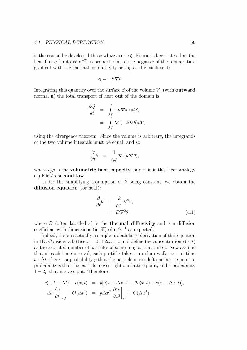
4.1. PHYSICAL DERIVATION 59

is the reason he developed those whizzy series). Fourier’s law states that theheat flux q (units Wm−2) is proportional to the negative of the temperaturegradient with the thermal conductivity acting as the coefficient:

q = −k∇θ.

Integrating this quantity over the surface S of the volume V , (with outwardnormal n) the total transport of heat out of the domain is

−dQdt

=

∫S

−k∇θ.ndS,

=

∫V

∇.(−k∇θ)dV,

using the divergence theorem. Since the volume is arbitrary, the integrandsof the two volume integrals must be equal, and so

∂

∂tθ =

1

cpρ∇.(k∇θ),

where cpρ is the volumetric heat capacity, and this is the (heat analogyof) Fick’s second law.

Under the simplifying assumption of k being constant, we obtain thediffusion equation (for heat):

∂

∂tθ =

k

ρcp∇2θ,

= D∇2θ, (4.1)

where D (often labelled κ) is the thermal diffusivity and is a diffusioncoefficient with dimensions (in SI) of m2s−1 as expected.

Indeed, there is actually a simple probabilistic derivation of this equationin 1D. Consider a lattice x = 0,±∆x, . . ., and define the concentration c(x, t)as the expected number of particles of something at x at time t. Now assumethat at each time interval, each particle takes a random walk: i.e. at timet+∆t, there is a probability p that the particle moves left one lattice point, aprobability p that the particle moves right one lattice point, and a probability1− 2p that it stays put. Therefore

c(x, t+ ∆t)− c(x, t) = p[c(x+ ∆x, t)− 2c(x, t) + c(x−∆x, t)],

∆t∂c

∂t

∣∣∣∣x,t

+O(∆t2) = p∆x2 ∂2c

∂x2

∣∣∣∣x,t

+O(∆x3),


upon taking appropriate Taylor expansions on each side. Now, if we identifyD = p∆x2/∆t, and take the limits of ∆x → 0 and ∆t → 0 such that Dremains finite, we recover the diffusion equation. Cool!

There are many, many fascinating properties of this equation, some ofwhich we will touch on in the later parts of this course. For the momenthowever, we will just note that to find a solution of this equation, we will needboundary conditions, and also initial conditions on the spatial distributionof θ(x, 0) = θ0(x) alone, since the equation is only first order in time. Thetechnique of separation of variables is still eminently useful for solving thisequation on finite domains, but there is another form of solution which canbe very useful, particularly at ‘early’ times, where the meaning of ‘early’ canbe quantified.

4.2 Similarity solutions & error functions

Let’s consider the simplest version of the diffusion equation with θ dependingon a single space variable x and t. Therefore, θ must satisfy

∂

∂tθ = D

∂2

∂x2θ, (4.2)

We can find a solution to this equation without applying boundary condi-tions by considering a a similarity variable η, defined as

η =x

2√Dt

.

Notice how this grouping is very suggestive of the grouping we found whenconstructing the diffusion equation from a random walk. This is no coinci-dence. Therefore,

∂

∂t=

∂η

∂t

∂

∂η=−x

4√Dt3

∂

∂η=−η2t

∂

∂η,

∂

∂x=

∂η

∂x

∂

∂η=

1

2√Dt

∂

∂η,

∂2

∂x2=

1

4Dt

∂2

∂η2.

Therefore, the heat equation can be reposed as a differential equationonly in η:

−η2t

(∂θ

∂η

)=

D

4Dt

∂

∂η

(∂θ

∂η

).

4.3. CARTESIAN GEOMETRY 61

With the substitution,

X =∂θ

∂η,

∂X

∂η= −2ηX,

logX = −η2 + C1,

X = C2e−η2

,

θ = C32√π

∫ x

2√Dt

0

e−u2

du,

= C3erf

[x

2√Dt

], (4.3)

where C1, C2 and C3 are related constants determined by the initial condi-tions and erf(y) is the error function. The error function erf(x/2

√Dt) is

plotted in the figure (for D = 1) for times t = 10−3, t = 10−2, t = 10−1, andt = 100.

• The error function is scaled so that erf(0) = 0 and erf(y) → ±1 asy → ±∞.

• The solution does not change along lines where x = A√Dt for A a

constant. This scaling is characteristic of diffusive processes.

• This derivation has no information from the boundary conditions. In-terestingly, it can be used as an early-time approximation to problemson finite domains with boundary conditions, until the solution ‘feels’the influence of the boundaries.

4.3 Cartesian geometry

To show this, consider the transient problem of diffusion on a finite bar oflength 2L. Assume that the initial conditions are that

θ(x, 0) =

{Θ0 0 < x ≤ L0 −L ≤ x < 0

,

while the boundary condition is that

θ(L, t) = Θ0,

θ(−L, t) = 0,

for all time.


−2 −1.5 −1 −0.5 0 0.5 1 1.5 2

−1

−0.8

−0.6

−0.4

−0.2

0

0.2

0.4

0.6

0.8

1

Figure 4.1: Plots (with D = 1) of the error function erf(x/2√Dt) for times

t = 10−3 (solid); t = 10−2 (dashed); t = 10−1 (dotted); and t = 100 (dot-dashed).


• This problem has inhomogeneous boundary conditions, which makeapplication of separation of variables problematic.

• The way to deal with this issue is to identify a steady solution whichsatisfies the boundary conditions.

• The steady solution must correspond to the late-time behaviour, whentransients have decayed, and must naturally satisfy the inhomogeneousboundary conditions,

∂

∂tθs = 0 =

∂2

∂x2θs,

θs(x) = Θ0(x+ L)

2L.

• Therefore, we can define a new variable θ (the transient component)with homogeneous boundary conditions and modified initial conditions,if we subtract this steady-state solution θs from θ:

θ(x, t) = θ(x, t)− θs(x),

θ(±L, t) = 0,

θ(x, 0) = Θ0

[H(x)− (x+ L)

2L

],

where H(x) is the Heaviside step function. ‘Clearly’, θ(x, 0) is odd.

Now applying the five-step algorithm as in section 3.2.1 for separation ofvariables to θ is straightforward:

1. Separate the variables:

θ(x, t) = X(x)T (t).

2. Therefore,

T = −DλT,X ′′ = −λX,

for some (positive) constant λ. Notice that the Sturm-Liouville oper-ator for the (spatial) function X is the same for the heat equation asfor the wave equation. This is unsurprising since they both involve the


Laplacian operator of course. As before, the solutions for X can beexpressed as

X(x) = A cos(√

λx)

+B sin(√

λx).

Applying the boundary conditions

X(−L) = 0→ A cos(√λL)−B sin(

√λL) = 0,

X(L) = 0→ A cos(√λL) +B sin(

√λL) = 0,

which implies that

λ =n2π2

L2,

A = 0,

for positive integer n, and so we have eigenvectors

Xn(x) = Bn sin[nπxL

].

3. Therefore,

Tn = −Dn2π2

L2Tn,

Tn = Cn exp

[−Dn

2π2

L2t

].

4. The general solution for θ is

θ(x, t) =∞∑n=1

bn sin[nπxL

]exp

[−Dn

2π2

L2t

],

which is fortunately also odd in x.


5. The initial condition is that∞∑n=1

bn sin[nπxL

]= Θ0

[H(x)− (x+ L)

2L

],

Lbm = Θ0

∫ L

0

sin(mπx

L

)dx

−Θ0

2

∫ L

−Lsin(mπx

L

)dx

−Θ0

2L

∫ L

−Lx sin

(mπxL

)dx,

= −LΘ0

mπcos(mπ) +

LΘ0

mπ

+LΘ0

mπcos(mπ)−

[Θ0L

2m2π2sin(mπx

L

)]L−L,

=LΘ0

mπ,

after a bit of good old-fashioned integration by parts. Therefore, thetransient solution and full solution are

θ = Θ0

∞∑n=1

1

nπsin(nπxL

)exp

(−n

2π2Dt

L2

),

θ =Θ0(x+ L)

2L+ Θ0

∞∑n=1

1

nπsin(nπxL

)exp

(−n

2π2Dt

L2

). (4.4)

Clearly, the transient solution decays to zero over time, but has a non-trivialcontribution initially. The full solution is plotted in the figure with thicklines for different times.

Fascinatingly, the error function is a valuable approximation for earlytimes (with t� L2/D). For an infinite domain with θ → Θ0 as x→∞, andθ → 0 as x→ −∞, the solution in terms of error functions (see the examplesheet) is

θi =Θ0

2

(1 + erf

[x

2√Dt

]). (4.5)

This is also plotted on the figure with thin lines (honestly). For the earlytimes, θi is indistinguishable from the full solution θ. Only for times whereθi is substantially different from 0 and Θ0 at the boundaries is it possible totell the difference. This occurs for times of the order of L2/D. Therefore,error function solutions can be very useful for early-time approximations.


−1 −0.8 −0.6 −0.4 −0.2 0 0.2 0.4 0.6 0.8 1

0

0.2

0.4

0.6

0.8

1

Figure 4.2: Plots (with L = 1 and D = 1 for simplicity) of θ/Θ0 as defined in(4.4) for: t = 0 (very thick line); t = 10−3 (thick solid line); t = 10−2 (thickdashed); t = 10−1 (thick dotted); t = 100 (thick dot-dashed). Also plottedis the error function approximation, as defined in (4.5) for: t = 10−3 (thinsolid line); t = 10−2 (thin dashed); t = 10−1 (thin dotted); t = 100 (thindot-dashed). Only the last line is visible.

4.4. ANNULAR GEOMETRY 67

4.4 Annular geometry

Of course, just as with the wave equation, separation of variables can beapplied to solve diffusion problems in more complicated geometry. A niceexample, which once again leads to Bessel’s equation (but now utilizes bothlinearly independent solutions) is to consider the problem of the transientwarming of the insulation material around a pipeline of finite cross-section.This is an (extremely simplified) model for a ground source heat pump, oneof the many ways that will allow society to reduce carbon emissions, andthus save what is left of the planet.

Consider an infinitely long pipeline of inner radius Ri and outer radiusRo > Ri, and thermal diffusivity D. This pipe is exposed to the ground at(constant) temperature Θg. At time t = 0+, a fluid is pumped through thepipeline which instantaneously heats up the inner wall of the pipe from Θg toa constant temperature Θf > Θg. We wish to calculate the time-dependentcross-sectional temperature distribution in the pipe. (In reality of course, theidea is to exchange heat between the fluid and the ground, and so the fixedinner boundary condition is not really what usually happens. This problemis quite complicated enough for the moment though!)

The problem is clearly axisymmetric, and so defining the scaled temper-ature distribution in the pipe as θ(r, t) such that

ψ(r, t) =Θ(r, t)−Θg

Θf −Θg

,

the problem reduces to

∂

∂tψ =

D

r

∂

∂r

(r∂

∂rψ

), ψ(Ri, t) = 1, ψ(Ro, t) = 0, ψ(r, 0) = 0, Ri < r < Ro.

As in the cartesian example in section 4.3, it is convenient to subdivide ψfurther into a steady state part ψs and a transient part ψ with homogeneousboundary conditions:

ψ(r, t) = ψs(r) + ψ(r, t), ψs(Ri) = 1, ψs(Ro) = 0,

d

drψs =

A

r,

ψs =log(r/Ro)

log(Ri/Ro).

Now, it is straightforward to follow our algorithm.


1. If we separate the variables, and hence assume that ψ(r, t) = R(r)T (t),we obtain

T = −λDT,r2R′′ + rR′ + λr2R = 0,

where the separation constant λ is of course the eigenvalue.

2. We now know that the R equation is just Bessel’s equation of zerothorder with appropriate rescaling of r (as shown in (3.5)) and so thegeneral eigenfunction is

Rm(r) = AmJ0(smr) +BmY0(smr), s2m = λm,

where the eigenvalues λm (and the relationship between Am and Bm,leaving an overall scaling free) are to be determined from the homo-geneous boundary conditions. Because the problem is defined in anannular region Ri < r < Ro, the Bm 6= 0, and the eigenfunction mustinvolve both J0 and Y0. Imposing the homogeneous boundary conditionψ(Ri, t) = 0 at r = Ri, we obtain

Rm(r) = am

[J0(smr)

J0(smRi)− Y0(smr)

Y0(smRi)

],

and thus the eigenvalue is quantized by the condition at r = Ro:

Y0(smRi)J0(smRo)− Y0(smRo)J0(smRi) = 0.

As is shown in the figure, this has an infinite number of solutions,(thank goodness, since this is an appropriate Sturm-Liouville system)and so am may be chosen (if we wish) to normalize the eigenfunctions.Notice that we know by construction (without needing to verify it, for-tunately) that the eigenfunctions are orthogonal on the interval [Ri, Ro]with respect to the weight function r:

am =

(∫ Ro

Ri

r

[J0(smr)

J0(smRi)− Y0(smr)

Y0(smRi)

]2

dr

)−1/2

.

3. The other separated solution can be straightforwardly constructed foreach eigenvalue, and so

Tm(t) = e−Ds2mt, ψm(r, t) = Tm(t)Rm(r).

4.4. ANNULAR GEOMETRY 69

0 10 20 30 40 50 60 70 80 90 100−0.05

0

0.05

Figure 4.3: Plot of Y0(smRi)J0(smRo) − Y0(smRo)J0(smRi) against sm forRi = 1 and Ro = 2. Clearly there are infinitely many solutions (intersectionswith the dashed line at 0).

4. Therefore, the general solution is

ψ(r, t) = ψs +∞∑m=1

Cme−Ds2mtRm(r),

clearly showing that ψ → ψs as t→∞.

5. All that remains is to determine the Cm. As before, the subdivision ofψ has made the initial condition on ψ

ψ(r, 0) = −ψs(r), ψ(r, 0) = ψ(r, 0) + ψs(r),

and so

Cn = −∫ Ro

Ri

rψsRn(r)dr,

and the problem is completely solved. Simples!

Exercise: Determination of flux

Determine the time-dependent heat flux into the ground. Can you expressit completely in terms of J1 and Y1 using the recursion relations listed insection 3.3.2?

Chapter 5

Laplace’s equation


Of course, not all problems are time-dependent, and sometimes we are partic-ularly interested in steady-state solutions. Indeed, we have already encoun-tered the fact that steady-state heat conduction problems require findingthe solution of one of the most important PDEs of all, Laplace’s equation,which in general form is

∇2ψ = 0,

in some domain D. This equation is obviously subject to given boundaryconditions on the boundary δD of D:

• If ψ is given on the boundary, (Dirichlet conditions) ψ has a uniquesolution;

• If n.∇ψ is given on the boundary, (Neumann conditions) ψ is uniqueup to an additive constant, since only normal gradients are given (n isthe outward normal of the boundary).

As we shall see, the form of the solution naturally varies with choice ofcoordinate system.

It is important to appreciate that Laplace’s equation does not just applyto steady state heat conduction! There are a huge number of situations whereit arises.

1. In incompressible fluid flow in a region in the absence of sources, sinks,and vortices (i.e. the flow is irrotational) the fluid velocity u can beexpressed as a velocity potential φ such that u = ∇φ, and so byincompressibility ∇2φ = 0.

71

72 CHAPTER 5. LAPLACE’S EQUATION

2. Indeed, the study of solutions to Laplace’s equation is often referredto as potential theory because there are many physical situationswhere a vector quantity (often a so-called conservative force) can beexpressed as the gradient of a potential, i.e.

F = −∇ψ,

the sign being conventional as it is reasonable that the force will actfrom regions of high potential to low potential. Such a force is calledconservative as the work done going round any closed path in a domainis zero: ∮

C

F.dr = 0.

Important examples include Newton’s (classical) gravitational force andthe electrostatic force (obeying Coulomb’s law). In such situations itis possible to define a force field (all sounds very Star Trek) suchas the gravitational field G or the electric field E. By consideringintegrals of these fields over the surface of arbitrary closed domains inthe absence of masses (for gravity) or charges (for electrostatics) andapplying the divergence theorem, it is straightforward to show that therelevant potentials in turn satisfy Laplace’s equation.

3. Harmonic functions (another name for solutions to Laplace’s equa-tions) are also extremely important in mathematics with no (obvious)requirement to think about physics. A truly beautiful example whichyou will discover in either Complex Methods or Complex Analysis (andhopefully both!) arises when a complex function f(z) is considered. Letus suppose f(z) is defined in some region R of the complex plane, wherez = x+ iy and

f(z) = u(x, y) + iv(x, y).

Therefore, the requirement that f is analytic in R (i.e. single-valuedand differentiable, loosely a generalization of the concept of continuityto complex functions) can be shown to require that u and v both satisfythe two-dimensional version of Laplace’s equation. Quite amazing.

So, Laplace’s equation is all over the place. How can we solve it? Separateand conquer!

5.2. 3D CARTESIAN COORDINATES 73

5.2 3D cartesian coordinates

In 3D cartesian space,

ψxx + ψyy + ψzz = 0,

and we assume that ψ(x, y, z) = X(x)Y (y)Z(z), and so Laplace’s equationbecomes

X ′′

X+Y ′′

Y+Z ′′

Z= 0.

As before, each ratio must be a constant, and so

X ′′ = −λlX,Y ′′ = −µmY,Z ′′ = (λl + µm)Z,

and we are expecting the eigenvalues λl and µm to be positive. (Also similarlyto before, it can be shown that the other sign choice is not consistent withthe boundary conditions.)

So, for a solution, we need to continue following the algorithm for sepa-ration of variables listed in section 3.2.1, adapted for the extra dimensions:

1. We have already separated the variables.

2. Find the eigenvalues λl and µm, and the associated eigenfunctionsXl(x), Ym(y) by applying boundary conditions on x and y.

3. Hence solve for the form of Zl,m(z), thus constructing a particular so-lution Plm = Xl(x)Ym(y)Zl,m(z).

4. Sum across all possible particular solutions to define a general solution

ψ(x, y, z) =∑l,m

almXl(x)Ym(y)Zl,m(z).

Note that there is no separate sum across the subscripts of Z: thisfunction is determined through the other two eigenvalues and associatedeigenvectors.

5. Determine the alm coefficients using the boundary conditions on z.

Of course, this approach becomes a lot clearer by considering an example.


5.2.1 Example: Steady heat conduction

Consider the problem of steady heat conduction in a semi-infinite rod withrectangular cross-section, heated at one end with fixed temperature (i.e.isothermal boundary conditions) on its other surfaces. So, without loss ofgenerality, we want to find the steady temperature field ψ(x, y, z)

∂

∂tψ = κ∇2ψ = 0,

ψ(x, y, 0) = Θ(x, y), ψ → 0 as z →∞,ψ(0, y, z) = ψ(a, y, z) = ψ(x, 0, z) = ψ(x, b, z) = 0.

1. Assume ψ = XlYmZl,m.

2. Solving X ′′ = −λlX, such that X(0) = X(a) = 0 implies that

λl =l2π2

a2, Xl =

√2

asin

(lπx

a

), l = 1, 2, 3 . . .

where the eigenfunction has been normalized by the square-root factor.(Can you see a connection with a Fourier sine series? This normaliza-tion is not necessary, as can be seen by comparison with the transientsolution considered in section 4.3.)

3. Similarly, solving Y ′′ = −µmY , such that Y (0) = Y (b) = 0 implies that

µm =m2π2

b2, Ym =

√2

bsin(mπx

b

), m = 1, 2, 3 . . .

4. Now solve for Z using the eigenvalues:

Z ′′ =

(l2π2

a2+m2π2

b2

)Z,

Z = α exp

[(l2

a2+m2

b2

)1/2

πz

]+ β exp

[−(l2

a2+m2

b2

)1/2

πz

].

Since ψ remains bounded as z →∞, α = 0 immediately.

5. Therefore, the general solution is

ψ(x, y, z) = (5.1)

2√ab

∞∑l=1

∞∑m=1

alm sin

(lπ

ax

)sin(mπby)

exp

[−(l2

a2+m2

b2

)1/2

πz

].

5.2. 3D CARTESIAN COORDINATES 75

6. The boundary condition at z = 0 now determines the coefficients alm,if we exploit the orthogonality of sine functions we discussed right atthe beginning of the course.

Θ(x, y) =2√ab

∞∑l=1

∞∑m=1

alm sin

(lπ

ax

)sin(mπby),

2√ab

∫ b

0

∫ a

0

Θ sin(pπax)

sin(qπby)dxdy

=∞∑l=1

∞∑m=1

alm

[2

b

∫ b

0

sin(mπby)

sin(qπby)dy

]×[

2

a

∫ a

0

sin

(lπ

ax

)sin(pπax)dx

],

=∞∑l=1

∞∑m=1

almδmqδlp,

= apq.

We thus have a simple form for the coefficients alm given a boundarycondition Θ(x, y).

• This solution is clearly closely related to a Fourier series.

• Indeed, discontinuities in the boundary conditions (for example on theline x = 0, z = 0, 0 < y < b) lead to solutions which take the meanvalue of the two boundary conditions there.

• There is no need to normalize the sine eigenfunctions (i.e. multiplythem by

√2/a or

√2/b) if you don’t want to. The rescaling naturally

passes through leading to the same values of the coefficients alm.

• The sine functions arise because of the homogeneous Dirichlet condi-tions. If we had insulating Neumann conditions, (e.g. ∂ψ/∂x = 0 atx = 0, a) we would expect cosine eigenfunctions in the x and y direc-tions.

• Furthermore, if the bar were finite, we would expect sinh and coshfunctions for Z upon applying the boundary conditions.

Solution for Θ = 1

An ‘easy-to-understand’ specific example is when Θ(x, y) = 1, and so the endis being kept at a constant temperature. Using (5.1) with the normalized


eigenfunctions, the coefficients are

apq =2√ab

∫ b

0

∫ a

0

sin(pπax)

sin(qπby)dxdy,

=2√ab

ab

π2pq[1− (−1)p] [1− (−1)q] ,

=

{8√ab

π2pqp, q both odd;

0 otherwise.

Therefore

ψ(x, y, z) = 16∞∑l=1

∞∑m=1

sin[

(2m−1)πyb

]sin[

(2l−1)πxa

]π2(2l − 1)(2m− 1)

exp[−kl,mπz],

k2l,m =

(2l − 1)2

a2+

(2m− 1)2

b2.

• The solution is unsurprisingly hotter in the middle.

• As z → ∞, the solution is dominated by the lower harmonics (i.e.where kl,m is small, and hence where l and m are small). Indeed, it isdominated by l = m = 1 for sufficiently large z.

• When a = b (i.e. in a square bar) km,l = kl,m, and the eigenvalues aredegenerate. But everything is still alright, as the eigenvectors are stillorthogonal. This is analogous to the situation with matrices of course.

5.3 Plane polar coordinates

In plane polar coordinates, ψ(r, θ), and Laplace’s equation becomes

∇2ψ = 0 =1

r

∂

∂r

(r∂

∂rψ

)+

1

r2

∂2

∂θ2ψ.

Follow the algorithm.

1. ψ = R(r)Θ(θ), such that

Θ′′ = −λΘ,r

R(rR′)

′= λ.

The separation constant λ is clearly an eigenvalue.

5.3. PLANE POLAR COORDINATES 77

2. Considering the equation for Θ, remember that Θ(θ + 2π) = Θ(θ).

• Therefore, for n a positive integer, λ = n2 is an eigenvalue withassociated eigenvector

Θn(θ) = an cosnθ + bn sinnθ.

• For n2 = 0 = λ,

Θ0(0) =a0

2+ b0θ =

a0

2,

by periodicity. (The particular scaling is just to show the similar-ity to Fourier series representations.)

3. We also need to treat λ = n2 > 0 and λ = 0 differently when deter-mining the associated function Rn(r).

• For n 6= 0,

r(rR′n)′ − n2Rn = 0.

Let us search for power law solutions, i.e. assume that Rn ∝ rβ.Therefore

β2 − n2 = 0 → β = ±n,Rn(r) = cnr

n + dnr−n, n = 1, 2, 3 . . .

and so the particular solution is

ψn(r, θ) = (an cosnθ + bn sinnθ)(cnrn + dnr

−n),

(One of the constants can be absorbed into a general scaling, butwe retain them all at this stage.)

• For n = 0,

(rR′0)′ = 0→ R0 = d0 log r + c0 = ψ0(r, θ),

since Θ0 is merely a constant.

4. Therefore, the general solution for Laplace’s equation in polar coordi-nates is

ψ(r, θ) = c0 + d0 log r +∞∑n=1

(an cosnθ + bn sinnθ)(cnrn + dnr

−n). (5.2)


It is important to remember that strictly speaking only three of an, bn,cn and dn are needed for a complete description, as one of the constantscan always be scaled into the others, or equivalently set to one. I haveretained all four so that we can deal easily with the different situations,(for example where cn = 0, or dn = 0).

5. Though there seem to be a terrifying number of different constants inthis expression, boundary conditions often simplify the problem sub-stantially.

• If the problem is defined on the interior of a disc (wlog the unitdisc), d0 = 0 = dn for the solution to be regular at the origin.

• Similarly, if the problem is defined on an infinite domain thatexcludes the origin (for example outside the unit disc) then thetypical requirement that ψ → ψ∞ (bounded) as r → ∞ impliesthat d0 = 0 = cn, (n > 0) and c0 = ψ∞.

• Life is much more fiddly in annular regions r1 < r < r2, (as wesaw when discussing the diffusion equation) where all the indepen-dent constants need to be determined by applying the boundarycondition on both the inner and outer limits. Remember however,that on these boundaries, the r-dependent components are justconstants.

• The constants of course are determined in the conventional wayby exploiting the orthogonality properties of sines and cosines. Itis easiest to understand by considering a specific example.

5.3.1 Example: Laplace’s equation in the unit disc

Solve Laplace’s equation for 0 < r < 1, such that ψ(1, θ) = f(θ), a givenfunction. By requiring regularity at the origin, (5.2) has d0 = 0, dn = 0,(n > 0) c0 = a0/2, and so

ψ(r, θ) =a0

2+∞∑n=1

(an cosnθ + bn sinnθ)rn.

When written in this form this should look awfully familiar, since at r = 1,

f(θ) = ψ(1, θ) =a0

2+∞∑n=1

(an cosnθ + bn sinnθ),

5.4. CYLINDRICAL POLAR COORDINATES 79

and we are just trying to find the coefficients of a Fourier series periodic on[0, 2π]. Therefore

an =1

π

∫ 2π

0

f(θ) cosnθdθ, bn =1

π

∫ 2π

0

f(θ) sinnθdθ.

Note that the influence of the higher harmonics (i.e. larger n) is localizednear r = 1 due to the rn factor.

5.4 Cylindrical polar coordinates

In this case, Laplace’s equation is

∇2ψ = 0 =1

r

∂

∂r

(r∂

∂rψ

)+

1

r2

∂2

∂θ2ψ +

∂2

∂z2ψ.

Follow the algorithm, paying particular attention to what we have just learntabout the closely related problem in plane polar coordinates.

1. ψ = R(r)Θ(θ)Z(z) such that

Θ′′ = −n2Θ,

Z ′′ = k2Z

rd

dr

(rd

drR

)+ (k2r2 − n2)R = 0,

using already the knowledge we have learnt that

Θn(θ) = an cosnθ + bn sinnθ,

which of course deals also with the case of n = 0, where due to period-icity we know that the term that is linear in θ should be zero.

2. We also see that Zk = cke−kz + dke

kz.

3. Finally, letting kr = z, the equation for R becomes Bessel’s equationof order n (can you show this?) and so

Rn = αnJn(kr) + βnYn(kr).

4. All these can be combined to form a general solution. We know that theeigenvalues k will be quantized by the boundary conditions into an in-finite set kj, and so the general solution in cylindrical polar coordinatesis

ψ(r, θ, z) =∞∑n=0

∞∑j=1

[αjnJn(kjr) + βjnYn(kjr)]

×[an cosnθ + bn sinnθ][cje−kjz + dje

kjz]. (5.3)


Pretty nasty eh?

5.4.1 Example: Heat conduction in an infinite wire

Consider the cylindrical generalization of the problem discussed in section5.2.1, and so consider the problem of steady heat conduction in a semi-infinite rod with circular cross-section of radius a, heated at one end (forsimplicity to a uniform and constant temperature) with fixed (i.e. isothermalboundary conditions) on its other surfaces. So, without loss of generality, wewant to find the steady temperature field ψ(r, θ, z)

∂

∂tψ = κ∇2ψ = 0,

ψ(r, θ, 0) = Θ0, ψ → 0 as z →∞,ψ(a, θ, z) = 0.

Because of the symmetry of the boundary conditions, the solution cannotdepend on θ, so bn = 0 = an for all n > 0 in (5.3). Similarly, all the djmust be zero because of the far field condition, and all the βjn must be zerobecause of the regularity of the solution at r = 0, and so

ψ(r, θ, z) =∞∑j=1

AjJ0

(kjr

a

)e−kjz/a,

Θ0 =∞∑j=1

AjJ0

(kjr

a

),

where the kj can now be identified as the zeroes of J0. The coefficients canbe simply calculated by using orthogonality relations.

Exercise: Calculation of Aj

By using orthogonality, and the recursion relations between J0 and J1 definedin section 3.3.2, show that the solution to this problem is

ψ(r, θ, z) =∞∑j=1

2Θ0

kjJ1(kj)J0

(kjr

a

)e−kjz/a.

5.5 Laplace’s equation in spherical polars

A classic piece of MYSAYK is the correct definition of spherical polar co-ordinates r, θ, φ. The spherical polar description of a point with cartesiandescription (x, y, z);

5.5. LAPLACE’S EQUATION IN SPHERICAL POLARS 81

• r is the distance from the origin, (equivalently the length of the positionvector r from [0, 0, 0] to [x, y, z]) and r ≥ 0;

• θ is the angle the position vector r makes with the positive z axis (i.e.θ = π/2− latitude in radians) and 0 ≤ θ ≤ π;

• φ is the angle the projection of the position vector onto the x−y planemakes with the positive x axis (i.e. φ is the longitude) and 0 ≤ φ < 2π.

• Therefore

x = r sin θ cosφ;

y = r sin θ sinφ;

z = r cos θ;

dV = r2 sin θdrdθdφ,

where dV is a volume element.

In spherical polar coordinates,

∇2ψ = 0,

1

r2

∂

∂r

(r2 ∂

∂rψ

)+

1

r2 sin θ

∂

∂θ

(sin θ

∂

∂θψ

)+

1

r2 sin2 θ

∂2

∂φ2ψ = 0.

In this course, we restrict attention to axisymmetric disturbances, and soψ = ψ(r, θ), independent of φ. So, just follow the algorithm.

1. Separating variables, under this assumption

ψ(r, θ) = R(r)Θ(θ).

2. Substituting this form into the governing equation, and multiplyingacross by r2/RΘ, we obtain

1

R

d

dr

(r2 d

drR

)+

1

Θ sin θ

d

dθ

(sin θ

d

dθΘ

)= 0,

([sin θ]Θ′)′+ λ[sin θ]Θ = 0, (5.4)(r2R′

)′ − λR = 0, (5.5)

where λ is of course a separation constant (the eigenvalue). we needto solve for the eigenvalues λ and the associated eigenfunctions Θ.The equation looks pretty tricky, but a cunning substitution yields aneat (and very important) solution, the Legendre polynomials (moreFMOTENC stuff again) as we now investigate.


5.5.1 Legendre’s equation

To solve (5.4), make the substitution x = cos θ. Since the problem is definedin general for 0 ≤ θ ≤ π, −1 ≤ x ≤ 1, and

d

dθ= − sin θ

d

dx.

Therefore, (5.4) becomes

− sin θd

dx

[sin θ

(− sin θ

d

dxΘ

)]+ λ sin θΘ = 0,

− d

dx

[(1− x2)

d

dxΘ

]= λΘ. (5.6)

This equation is in classic Sturm-Liouville form, and comparing with (2.12),p = 1− x2, q = 0, and w = 1. It is known as Legendre’s equation.

5.5.2 Legendre polynomials

We require a bounded solution of (5.6) on [−1, 1]. Let us seek a series solution

Θ =∞∑n=0

anxn.

Substituting this form into (5.6), we obtain

(1− x2)d2

dx2Θ− 2x

d

dxΘ + λΘ = 0,

(1− x2)∞∑n=2

ann(n− 1)xn−2 − 2∞∑n=1

annxn + λ

∞∑n=0

anxn = 0.

Considering the coefficient of xn,

0 = an+2(n+ 2)(n+ 1)− n(n− 1)an − 2nan + λan,

an+2 =

[n(n+ 1)− λ

(n+ 1)(n+ 2)

]an. (5.7)

Since this is a recursion relation relating an+2 to an, we can generate twolinearly independent solutions Le and Lo:

1. Le has a0 6= 0, a1 = 0;

2. Lo has a0 = 0, a1 6= 0


and so

Le = a0

[1 +

(−λ)x2

2!+

(−λ)(6− λ)x4

4!+

(−λ)(6− λ)(20− λ)x6

6!+ . . .

],

Lo = a1

[x+

(2− λ)x3

3!+

(12− λ)(2− λ)x5

5!+ . . .

].

But (5.7) implies that an+2/an → 1 as n → ∞ and so the (infinite) seriesconverges for |x| < 1, but not necessarily at |x| = 1. Indeed, the seriesdiverges at x = ±1. Therefore, the only way for the solution to remainbounded is for the series to terminate and so λ = m(m + 1) for someinteger m, thus defining the appropriate eigenvalue: cool eh?

Then for a given λ = m(m + 1), the series solution found is a (finite)polynomial (the Legendre polynomial of degree m, Pm(x)) associatedwith the eigenvalue λ = m(m + 1), defined by the terminating recursionrelation (5.7).

5.5.3 Properties of Legendre polynomials

The Legendre polynomials have many groovy properties.

• By convention, they are not normalized so∫ 1

−1

P 2m(x)dx 6= 1.

• Rather, the polynomials are scaled so that Pm(1) = 1.

• As is apparent in the figure, each Pn(x) has n zeroes in [−1, 1].

• When n is odd, Pn(x) is odd about x = 0.

• When n is even, Pn(x) is even about x = 0.

• The first five Legendre polynomials are plotted in the figure, and are

m = 0 λ = 0 P0(x) = 1;m = 1 λ = 2 P1(x) = x;

m = 2 λ = 6 P2(x) = 3x2−12

;

m = 3 λ = 12 P3(x) = 5x3−3x2

;

m = 4 λ = 20 P4(x) = 35x4−30x2+38

.

(5.8)


−1 −0.8 −0.6 −0.4 −0.2 0 0.2 0.4 0.6 0.8 1

−1

−0.8

−0.6

−0.4

−0.2

0

0.2

0.4

0.6

0.8

1

Figure 5.1: Legendre polynomials P0(x) (thin solid line); P1(x) (thick solid);P2(x) (dashed); P3(x) (dotted); P4(x) (dot-dashed).


• The Legendre polynomials are orthogonal since they are eigenfunctionsof a Sturm-Liouville system, i.e.∫ 1

−1

Pn(x)Pm(x)dx = 0, m 6= n.

• (Indeed, they are a great archetype of a class of orthogonal polynomial:other examples commonly arise in physics and engineering.)

• Due to the convention that Pn(1) = 1, (as shown on the example sheet,and also derived below in section 5.5.5):∫ 1

−1

P 2ndx =

2

2n+ 1.

• Bounded functions defined on [−1, 1] can be represented using the Leg-endre polynomials as a basis, i.e.

f(x) =∞∑n=0

anPn(x),

an =(2n+ 1)

2

∫ 1

−1

f(x)Pn(x)dx.

5.5.4 General axisymmetric solution

Now revisiting our algorithm:

1. ψ(r, θ) = R(r)Θ(θ).

2. Θn(θ) = Pn(x) = Pn(cos θ), with λ = n(n+ 1).

3. Therefore (5.5) becomes

(r2R′n)′ − n(n+ 1)Rn = 0.

Assuming that Rn ∝ rβ,

β(β + 1) = n(n+ 1),

β = n, or β = −(n+ 1).

Therefore, a particular solution is

ψn(r, θ) =(anr

n + bnr−(n+1)

)Pn(cos θ).


4. And so, the general axisymmetric solution is

ψ(r, θ) =∞∑n=0

(anr

n + bnr−(n+1)

)Pn(cos θ). (5.9)

5. As before, the constants an are determined by applying boundary con-ditions exploiting orthogonality of the Legendre polynomials. It is crit-ical to remember the 2/(2n + 1) factor, and also to be careful withthe actual argument of the functions, (i.e. remembering the differencebetween x = cos θ, and θ: obvious yes, but it can happen, trust me. . . ).

• If the problem is defined on the interior of a sphere (wlog the unitsphere), bn = 0 for the solution to be regular at the origin.

• Similarly, if the problem is defined on an infinite domain thatexcludes the origin (for example outside a sphere) then the typicalrequirement that ψ → ψ∞ (bounded) as r → ∞ implies thatan = 0, for n > 0 and a0 = ψ∞.

• Complications in this geometry correspond to solving problemsbetween shells r1 < r < r2, where both an and bn are in generalnon-zero, and the coefficients need to be determined by applyingthe boundary condition on both the inner and outer sphericalshell.

As before it is easiest to understand by considering specific examples.

Example: Laplace’s equation inside the unit sphere

Find the solution to Laplace’s equation inside the unit sphere, subject to anaxisymmetric boundary condition on r = 1, i.e. ψ(1, θ) = f(θ). Of course,we immediately have from the general solution (5.9) that bn = 0 to imposeregularity at the origin. Therefore, at r = 1, we have

f(θ) =∞∑n=0

anPn(cos θ), 0 ≤ θ ≤ π,

F (x) =∞∑n=0

anPn(x), x = cos θ, −1 ≤ x ≤ 1,

an =(2n+ 1)

2

∫ 1

−1

F (x)Pn(x)dx,

where f(θ) has been reposed as a F (cos θ) = F (x), i.e. as a function of cos θ.(See the example sheet for a more detailed calculation.)


5.5.5 Generating function

There are many, many beautiful properties of these polynomials (and indeedof other classes of orthogonal polynomials) several of which are discussedon the example sheet. Many of these properties are derived by exploitingthe uniqueness of solutions to Laplace’s equation. A particularly groovy ex-ample is the generating function for the Legendre polynomials (definitelyattractive, because it reduces the need for memorization)!

Consider the following problem. There is a unit point charge one unitaway from the origin along the positive z-axis. The potential ψ(r, θ) at anarbitrary point r, θ with r < 1 (PYSAYK now I’d say) is

ψ(r, θ) =1

ρ,

=1√

1− 2r cos θ + r2,

since

ρ = r− z,

ρ2 = |ρ|2 = r · r− 2r · z + z · z,= r2 − 2r cos θ + 1.

But

• ψ satisfies Laplace’s equation;

• It must be regular near the origin;

• And so, from uniqueness and (5.9) with bn = 0

1√1− 2r cos θ + r2

=∑n=0

anPn(cos θ)rn,

1√1− 2rx+ r2

=∑n=0

anPn(x)rn.

Note how easy it is here to transfer from functional dependence on cos θto functional dependence on x. Now make the assumption that Pn(1) = 1is our scaling requirement on the Legendre polynomials. Since they are theeigenfunctions of a self-adjoint operator, we know they are orthogonal, butwe do not yet know the scaling (consistent with Pn(x) = 1) of

In =

∫ 1

−1

P 2n(x)dx.


However, when x = 1 we obtain

1

1− r=

∑n=0

anrn → an = 1,

and so, amazingly∞∑n=0

Pn(x)rn =1√

1− 2rx+ r2, (5.10)

defining the generating function for the Legendre polynomials. Note thatthis function is a very elegant way to calculate the Legendre polynomials, as

1

n!

dn

drn

[1√

1− 2rx+ r2

]r=0

= Pn(x).

We can also obtain the scaling of the Legendre polynomials if we squareboth sides and integrate from −1 to 1.∫ 1

−1

dx

1− 2rx+ r2=

∞∑m=0

rm∞∑n=0

rn∫ 1

−1

Pn(x)Pm(x)dx,

=∞∑n=0

Inr2n,

=1

2r

∫ 2r

−2r

dy

1 + r2 − y, y = 2rx;

=−1

2rlog(1 + r2 − y)

∣∣∣∣2r−2r

,

=1

2r

[log(1 + r2 + 2r)− log(1 + r2 − 2r)

],

=1

rlog

(1 + r

1− r

),

=∞∑n=0

2

2n+ 1r2n,

using the series expansion for log(1 ± r) for r < 1 (MYSAYK if ever I sawit). Comparing both expressions, we obtain

In =

∫ 1

−1

P 2n(x)dx =

2

2n+ 1,

establishing (in a different way from the example sheet) the orthogonalityscaling condition for the Legendre polynomials subject to the requirementthat Pm(1) = 1.


• As an exercise, you should convince yourself that this works . . .

• Considering the potential response to a unit point charge is very remi-niscent of the approach used to construct Green’s functions, and indeedit is possible to generalize the concept of Green’s functions to PDEs: aproblem we will return to in the last part of the course.

5.5.6 An example with an unbounded far field

Consider a neutral conducting sphere (with radius r0) placed in a previouslyuniform electric field. Find the new perturbed electrostatic potential V . Re-member PYSAYK: the electric field E is minus the gradient of the potentialV , and V satisfies Poisson’s equation (FMOTENC again: essentially theforced generalization of Laplace’s equation);

E = −∇V, ∇2V = − ρ

ρ0

= 0,

where the charge density is ρ. In this particular problem, since the externalcharge density is zero, the equation thankfully reduces to Laplace’s equationagain.

Since V satisfies Laplace’s equation, and the problem is axisymmetric,(5.9) applies, and so

V (r, θ) =∞∑n=0

(anr

n +bnrn+1

)Pn(cos θ).

We need to be very careful with matching the conditions. In the far field (asr →∞) V must tend to its far field value, and so, wlog

V → −E0z = −E0r cos θ = −E0rP1(cos θ),

since P1(x) = x. Therefore, we have that

a1 = −E0, an = 0 for n = 0, n > 1,

showing that it is perfectly possible to deal with an unbounded far fieldsolution. Without loss of generality, we have chosen the origin so that θ = π/2is the level of zero potential.

‘Obviously’, the surface of the sphere r = r0 has zero potential, since itis neutral and conducting. Therefore,

V (r0) =b0r0

+

(b1r20

− E0r0

)P1(cos θ) +

∞∑n=2

bnPn(cos θ)

rn+10

= 0.


This must hold over the whole surface of the sphere, and so for all θ. There-fore, b0 = 0 = bn for n ≥ 2, while b1 = E0r

30, and so remembering P1(cos θ) =

cos θ,

V = −E0r cos θ

(1− r3

0

r3

).

5.5.7 Connection with Electrostatic multipoles

The Legendre polynomials are the natural mathematical description of ax-isymmetric electrostatic potentials. Consider charges placed nonuniformlybut axisymmetrically inside a sphere. Far away, the electrostatic potential(which in the absence of a far field should drop to zero, and so an = 0)satisfies

V (r, θ) =∞∑n=0

bnr−(n+1)Pn(cos θ).

• The term with n = 0 leads to

V ∝ b0r,

i.e. the potential for an (isotropic) monopole field from a point charge,or equivalently the field due to the total net charge concentrated atr = 0. (Yet again, doesn’t this really sound like a Green’s function?)

• The term with n = 1 leads to

V ∝ b1 cos θ

r2,

i.e. the potential for a dipole field induced by +q and −q charges closetogether.

• For n = 2,

V ∝ b2(3 cos2 θ − 1)

2r3,

i.e. the potential for a quadropole field equivalent to the field from fouralternating symmetrically placed charges.

Indeed, higher and higher values of n are associated with higher order mul-tipoles with increasingly complicated θ-dependent charge distributions.

Part III

Inhomogeneous ODEs& Fourier Transforms

91

Chapter 6

Generalized functions

6.1 Definition of the δ-function

This part of the course principally considers solution methods for second-order ODEs on both finite and infinite domains, though many of the funda-mental ideas can be generalized to PDEs, as we see in the last part of thecourse. To develop new techniques, new tools are unsurprisingly needed, andone of the most useful is the concept of a generalized function. Thesebeasts can be put on a rigorous footing, but here only their vital character-istics will be postulated, and accepted on faith. You don’t want to do toomuch worrying about epsilons and deltas and neighbourhoods and such-likeat the moment . . . .

Define the Dirac δ-function by its properties:

δ(x− ξ) = 0, ∀x 6= ξ,

∫ ∞−∞

δ(x− ξ)dx = 1. (6.1)

The δ-function may be thought of as a spike in the vicinity of x = ξ. Inparticular, if f(x) is continuous in the neighbourhood of x = ξ, then∫ ∞

−∞f(x)δ(x− ξ)dx = f(ξ). (6.2)

This is known as the sampling property.The δ-function can be put on a more rigorous footing by using ‘distribu-

tions’. One can think of the δ-function as a limit of a sequence of continuousfunctions Pn(x) such that, as n→∞, Pn(x)→ 0 ∀x 6= 0, and∫ ∞

−∞Pn(x) = 1.

93

94 CHAPTER 6. GENERALIZED FUNCTIONS

−1 0 1−5

0

5

10

15

20

−1 0 1−5

0

5

10

15

20

−1 0 1−5

0

5

10

15

20

Figure 6.1: Pn(x) for the top-hat, the Gaussian, and sin(nx)/(πx), showingconvergence towards the δ-function, for n = 2, 4, 8, 16, 32 (thin solid, dashed,dotted, dot-dashed, thick solid).

6.2. PROPERTIES OF THE δ-FUNCTION 95

The particular choice of Pn(x) is non-unique, and some examples are as shownin the figure:

Pn(x) =

{n2|x| < 1

n;

0 otherwise,

=n√πe−n

2x2

,

=sin(nx)

πx.

6.2 Properties of the δ-function

The δ-function has many useful properties, some of which you are asked toprove on the example sheet.

1. If f(x) is continuous in the neighbourhood of x = ξ, then∫ b

a

f(x)δ(x− ξ)dx =

{f(ξ) a < ξ < b;

0 otherwise.(6.3)

This is known as the sampling property. (This property shows thatthe δ-function is actually a functional: a function of a function. Ef-fectively, δ(x) takes as input a function f(x), and gives as output anumber f(0).)

2. If a 6= 0,

δ(at) =1

|a|δ(t), (6.4)

the scaling property.

3. Indeed, if the function f(x) has simple zeroes at n isolated points xi,i = 1, . . . n,

δ(f(x)) =n∑i=1

δ(x− xi)|f ′(xi)|

.

4. Provided g(x) is a function continuous in the vicinity of x = 0,

g(x)δ(x) = g(0)δ(x)


are equivalent generalized functions (e.g. they behave the same withrespect to the scaling and sampling properties). A specific importantexample of this is xδ(x) = 0, and so

yx = 1→ y =1

x+ cδ(x), (6.5)

for c an undetermined constant. This strange property is very usefulfor analysis of the ‘Heaviside step-function’, which naturally arises asthe integral of the δ-function.

5. The integral of the δ-function:∫ x

−∞δ(ξ)dξ =

{0 x < 01 x > 0

,

H(x) =

{0 x < 0;1 x > 0

, (6.6)

defining the Heaviside step-function as the integral of the δ-function,and so H ′(x) = δ(x). Often (because of the properties of Fourier rep-resentations for example) H(0) = 1/2 by definition.

6. The δ-function clearly has a ‘worse’ or ‘stronger’ discontinuity than theHeaviside step-function. If you’re a natural pessimist, even worse dis-continuities can be represented by derivatives of the δ-function, whichcan be defined by integrating the sampling property by parts:∫ ∞−∞

δ′(x− ξ)f(x)dx = [δ(x− ξ)f(x)]∞−∞ −∫ ∞−∞

δ(x− ξ)f ′(x)dx,

= 0− f ′(ξ),provided f has a continuous derivative at x = ξ.

7. Indeed, provided f(x) is sufficiently smooth at x = ξ:∫ ∞−∞

f(x)δ(n)(x)dx = (−1)nf (n)(0).

6.2.1 Example using properties of δ-function

Compute

I =

∫ ∞0

δ′(x2 − 1)x2dx.

To use properties, make the substitution u = x2. Therefore

I =1

2

∫ ∞0

δ′(u− 1)u1/2du =−1

2

[1

2u1/2

]u=1

=−1

4.

6.3. FOURIER SERIES OF δ-FUNCTION 97

6.3 Fourier series of δ-function

Consider the periodic function (known as the Dirac comb, very important insignal processing):

f(x) = δ(x), −L < x < L.

Formally, it is possible to write down a Fourier series representation

f(x) =∞∑

n=−∞

cneinπxL ,

cn =1

2L

∫ L

−Lf(x)e

−inπxL dx,

=1

2L

∫ L

−Lδ(x)e

−inπxL dx =

1

2L,

→ f(x) =1

2L

∞∑n=−∞

einπxL .

But since the δ-functions don’t overlap,

f(x) =∞∑

m=−∞

δ(x− 2mL),

and so finally, what is rather confusingly (as we shall see) called Poisson’sintegral formula is obtained

∞∑m=−∞

δ(x− 2mL) =1

2L

∞∑n=−∞

einπxL . (6.7)

6.3.1 Resolution of Fourier series problem

Now, the problem with the function shown in figure 1.3.2 can be understood.Here, f(x) is a periodic function with period 2 such that f(x) = 1 for 0 <x < 1 and f(x) = −1 for −1 < x < 0. Therefore, its derivative f ′(x) can be


expressed as

f ′(x) = 2∞∑

m=−∞

[δ(x− 2m)− δ(x− 1− 2m)] ,

=∞∑

n=−∞

einπx[1− e−inπ

],

=∞∑

n=−∞

einπx[1 + (−1)n+1

],

= 2∞∑m=0

[eiπx(2m+1) + e−iπx(2m+1)

],

= 4∞∑m=0

cos([2m+ 1]πx),

exactly as observed before. Which strikes me as pretty cool.

6.3.2 Eigenfunction expansion of δ-function

Now with the definition (and properties) of a δ-function, we can revisit themysteries of Sturm-Liouville theory as discussed in section 2.4, and in par-ticular express a δ-function as an eigenfunction expansion. Clearly, on aninterval [a, b] δ(x − ξ) satisfies homogeneous boundary conditions providedξ is not at the boundary. Therefore, from property 4, the δ-function has aneigenfunction expansion

δ(x− ξ) =∞∑n=1

CnYn(x),

Cm =

∫ b

a

w(x)Ym(x)δ(x− ξ)dx,

= w(ξ)Ym(ξ).

Since

w(x)

w(ξ)δ(x− ξ) = δ(x− ξ),

there are two equivalent eigenfunction expansions for δ(x− ξ):

δ(x− ξ) =∞∑n=1

w(ξ)Yn(x)Yn(ξ) =w(x)

w(ξ)

∞∑n=1

w(ξ)Yn(x)Yn(ξ),

=∞∑n=1

w(x)Yn(x)Yn(ξ). (6.8)

6.3. FOURIER SERIES OF δ-FUNCTION 99

This definition is also consistent with the sampling property, since, for afunction g(x) continuous in the vicinity of x = ξ:

g(x) =∞∑m=1

DmYm(x)(by completeness);∫ b

a

g(x)δ(x− ξ)dx =∞∑m=1

∞∑n=1

DmYn(ξ)

∫ b

a

w(x)Yn(x)Ym(x)dx,

=∞∑m=1

DmYm(ξ) = g(ξ),

by orthonormality. As we see below, this eigenfunction expansion for the δ-function can be related in a very natural way to the eigenfunction expansionfor the ‘Green’s function’ constructed in (2.25). As a particularly simpleexample, if L = −d2/dx2, w(x) = 1 and y(0) = y(L) = 0, it is straightforwardto establish (can you do it?) that

δ(x− ξ) =2

L

∞∑n=1

sin[nπxL

]sin

[nπξ

L

].

Chapter 7

Green’s functions

7.1 Green’s functions for BVPs

Now that we have defined the concept of a δ-function, we have a very naturalway to deifine the concept of a ‘Green’s function’ which we have encounteredseveral times before, in particular as we defined in terms of eigenfunctionsin section 2.5. Consider a linear second-order differential operator L, (of theform defined in (2.1)) on [a, b], i.e.

Ly(x) = α(x)d2

dx2y + β(x)

d

dxy + γ(x)y = f(x), (7.1)

where α, β, γ are continuous, f(x) is bounded, and α is nonzero (exceptperhaps at a finite number of isolated points), and a ≤ x ≤ b (which maytend to −∞ or +∞). For this operator L, the Green’s function G(x; ξ) isdefined as the solution to the problem

LG = δ(x− ξ), (7.2)

satisfying homogeneous boundary conditions G(a; ξ) = G(b; ξ) = 0.Therefore, the solution to the inhomogeneous problem Ly = f(x) with

homogeneous boundary conditions y(a) = y(b) = 0 is

y(x) =

∫ b

a

G(x; ξ)f(ξ)dξ. (7.3)

G is a kernel, and acts as an inverse to the differential operator L. Indeed Gdepends on L, but not the forcing function f , and once G is determined, weare able to work out particular integral solutions for any f(x), directly fromthe integral formulation (7.3).

101

102 CHAPTER 7. GREEN’S FUNCTIONS

We can easily establish that (7.3) is a simple consequence of (7.2) andthe sampling property (6.3):

L∫ b

a

G(x; ξ)f(ξ)dξ =

∫ b

a

LGf(ξ)dξ,

=

∫ b

a

δ(x− ξ)f(ξ)dξ = f(x),

y(a) =

∫ b

a

G(a; ξ)f(ξ)dξ = 0 =

∫ b

a

G(b; ξ)f(ξ)dξ = y(b).

7.2 Construction of the Green’s function

The direct construction (i.e. without recourse to eigenfunctions, though ofcourse the two approaches are completely equivalent) of the Green’s functionis highly algorithmic, and relies on the fact that away from x = ξ, LG = 0,and so G must depend on solutions to the homogeneous equation. A sensibleway to proceed is:

1. Construct a general solution for x < ξ from two linearly independentsolutions y1(x) and y2(x) to the homogeneous problem Ly = 0, and so

G(x; ξ) = A(ξ)y1(x) +B(ξ)y2(x), a ≤ x < ξ.

A and B are independent of x, but typically dependent on ξ.

2. Construct a general solution for x > ξ from two linearly independentsolutions Y1(x) and Y2(x) to the homogeneous problem Ly = 0, (whichmay not be exactly the same as y1 and y2 as we shall see, becauseother choices may be more convenient) so

G(x; ξ) = C(ξ)Y1(x) +D(ξ)Y2(x), ξ < x ≤ b.

Similarly, C and D are independent of x, but typically are dependenton ξ. There are thus four constants, (A, B, C, and D) which need fourconditions to determine G uniquely.

3. Apply the homogeneous boundary condition at x = a to eliminateeither A or B, since

G(a; ξ) = 0 = Ay1(a) +By2(a).

7.2. CONSTRUCTION OF THE GREEN’S FUNCTION 103

4. Similarly, apply the homogeneous boundary condition at x = b to elim-inate either C or D, since

G(b; ξ) = 0 = CY1(b) +DY2(b).

5. The two remaining conditions are unsurprisingly associated with theproperties at the point x = ξ. G(x, ξ) must be continuous there,(proved below) and so

Ay1(ξ) +By2(ξ) = CY1(ξ) +DY2(ξ).

6. The final, fourth condition is the jump condition, which is the require-ment that [

dG

dx

]x=ξ+x=ξ−

=1

α(ξ),

limx→ξ+

dG

dx− lim

x→ξ−

dG

dx=

1

α(ξ),

→ CY ′1(ξ) +DY ′2(ξ)− Ay′1(ξ)−By′2(ξ) =1

α(ξ),

where α(x) is the coefficient of the second derivative in the operatorL as defined in (2.1). Often, (but not always, particularly in ex-aminations) the operator is posed so that α(x) = 1. You need to bevery careful also about the right hand side of (7.2): everything here as-sumes that the right hand side is +1×δ(x−ξ). If the equation is scaleddifferently, you need to make sure the rescaling is applied appropriately.

7. With these conditions the Green’s function is constructed, and then fora given forcing function f(x), the solution to the forced problem withhomogeneous boundary conditions y(a) = 0 = y(b) is

y(x) = Y1(x)

∫ x

a

C(ξ)f(ξ)dξ + Y2(x)

∫ x

a

D(ξ)f(ξ)dξ

+ y1(x)

∫ b

x

A(ξ)f(ξ)dξ + y2(x)

∫ b

x

B(ξ)f(ξ)dξ.

This last step is perhaps a little counter-intuitive, as the solution (involvingC and D) constructed by imposing the boundary condition at b is in theintegral with limits [a, x]. But remember for ξ in this range, x > ξ, whichwas the range where we constructed the solution involving C and D. Also,the integral allows x to run all the way up to b. Nevertheless, this is astraightforward, step-by-step algorithm for building a Green’s function.


7.2.1 Conditions at x = ξ

Understanding the condition of continuity at x = ξ is easiest by proceedingby contradiction.

• Assume that G is discontinuous there.

• The weakest possible discontinuity is a finite jump.

• Therefore,

d

dxG ∝ δ(x− ξ), d2

dx2G ∝ δ′(x− ξ).

• However, there is no discontinuity of that strength in (7.2).

• The initial assumption of at least a finite jump must be wrong.

• So G is continuous at x = ξ.

The jump condition (which shows that the Green’s function is not smoothat x = ξ) follows from integrating (7.2) over an arbitrarily small interval.Therefore∫ ξ+ε

ξ−εδ(x− ξ)dx, =

∫ ξ+ε

ξ−εα(x)

[d2

dx2G

]dx+

∫ ξ+ε

ξ−εβ(x)

[d

dxG

]dx

+

∫ ξ+ε

ξ−εγ(x)Gdx,

T4 = T1 + T2 + T3.

• By the properties of the δ-function, T4 = 1 whatever the positive valueof ε.

• Since G is continuous, and γ is bounded, T3 → 0 as ε→ 0.

• Since dG/dx is bounded, and β is bounded, T2 → 0 as ε→ 0.

• As α is continuous, α(x)→ α(ξ) as ε→ 0. Therefore, as ε→ 0,

T1 → α(ξ) limε→0

∫ ξ+ε

ξ−ε

[d2

dx2G

]dx = α(ξ)

[d

dxG

]x=ξ+x=ξ−

,

and the jump condition is established.


7.2.2 Example of construction of a Green’s function

It is of course instructive to consider an example. Consider the problem

−y′′ − y = f(x), y(0) = y(1) = 0.


1. For 0 ≤ x < ξ, G′′ +G = 0, which suggests G = A cosx+B sinx.

2. For ξ < x ≤ 1, G′′ +G = 0, which suggests (to me at least)

G = C cos(1− x) +D sin(1− x).

Why choose these? Remember this can be reposed in terms of the‘obvious’ choice as

G = (C cos 1 +D sin 1) cosx+ (C sin 1−D cos 1) sinx,

= C cosx+ D sinx.

The reason for the original choice involving (1−x) is convenience, anda likelihood to avoid error, for which your supervisor, your examiner,(and probably your DoS) will thank you.

3. Applying the boundary condition G(0, ξ) = 0 implies A = 0.

4. Applying the boundary condition G(1, ξ) = 0 implies C = 0 (nice andneat eh?) or, if you insist C = −D tan 1 (quite fiddly: and it will onlyget worse with the next two conditions . . . you have been warned . . . )

5. Therefore,

G(x; ξ) =

{B sinx 0 < x < ξ;

D sin(1− x) ξ < x < 1.

Applying the continuity condition,

B = Dsin(1− ξ)

sin ξ.

6. Therefore,

G(x; ξ) =

{D sin(1−ξ) sinx

sin ξ0 < x < ξ;

D sin(1− x) ξ < x < 1.


In the operator α(x) = −1 (careful!) for all x, and so the jump condi-tion is that

D [− cos(1− x)]ξ+ −D[

sin(1− ξ) cosx

sin ξ

]ξ−

= −1,

→ D =sin ξ

sin 1,

which then means the Green’s function is specified as

G(x; ξ) =

{sin(1−ξ) sinx

sin 10 < x < ξ;

sin(1−x) sin ξsin 1

ξ < x < 1.

7. And so we are able to construct the complete solution to −y′′−y = f(x)as

y(x) =sin(1− x)

sin 1

∫ x

0

f(ξ) sin ξdξ +sinx

sin 1

∫ 1

x

f(ξ) sin(1− ξ)dξ.

There are some useful points to bear in mind.

• Note the symmetry of G with respect to x and ξ.

• Indeed, for the two linearly independent solutions y1 = sin(x) andy2 = sin(1− x) of the homogeneous equation Ly = 0 which satisfy theboundary conditions at a and b respectively, note that the solution is

G(x; ξ) =y1(x)y2(ξ)H(ξ − x) + y2(x)y1(ξ)H(x− ξ)

J(y1, y2),

J(y1, y2) = α(x)W (y1, y2) = α(x)[y1(x)y′2(x)− y2(x)y′1(x)],

where J(y1, y2) is the conjunct (and W is the Wronskian of course,MYSAYK) which can be shown (can you?) to be a (nonzero) constantprovided the two solutions are linearly independent, and the differentialoperator is self-adjoint. Indeed, for homogeneous boundary conditions,this expression is an entirely equivalent (and potentially very quick)formula to construct the Green’s function.

• Be careful with the ξ < x region and ξ > x region when substitutinginto the integral.

• The homogeneous boundary conditions are essential to the constructionof the Green’s function, but problems with inhomogeneous boundary


conditions can be easily dealt with. This is essentially a method toconstruct a particular integral with homogeneous boundary conditions.It is easy to build a complementary function (i.e. a solution of thehomogeneous equation) with inhomogeneous boundary conditions andthen add this to the Green’s function, since the operator is linear.

• As an example of this consider the problem with inhomogeneous bound-ary conditions

−y′′ − y = f(x), y(0) = 0, y(1) = 1.

The complementary function is C1 cosx + C2 sinx, and the boundaryconditions imply C1 = 0, C2 = 1/ sin 1. This solution can be combinedwith the calculated Green’s function solution to yield the solution tothe full, forced problem

y(x) =sinx

sin 1

+sin(1− x)

sin 1

∫ x

0

f(ξ) sin ξdξ +sinx

sin 1

∫ 1

x

f(ξ) sin(1− ξ)dξ.

7.2.3 Equivalence of eigenfunction expansion

Of course, this constructed Green’s function must be equivalent to the eigen-function expansion form derived in section 2.5, although it is by no meansalways immediately apparent that the two representations are equivalent. Inthe nomenclature of section 2.5, the general equation (2.21) is compatiblewith the problem described above when a = 0, b = 1, L = −d2/dx2, w = 1and λ = 1. This is consistent with the underlying assumptions requiredfor the eigenfunction expansion, since the eigenvalues of this operator areclearly λn = n2π2, (and so definitely never equal to λ = 1) with associated(orthonormal) eigenfunctions Yn(x) =

√2 sin(nπx).

Therefore, the Green’s function according to (2.25) for this problem is

Ge(x; ξ) = 2∞∑n=1

sin(nπx) sin(nπξ)

n2π2 − 1.

It is not at all obvious that this is the same Green’s function (the subscripte just labels this eigenfunction form for the Green’s function) as the one


described above. Indeed, for the two representations to be equivalent,

Ge(x; ξ) =sin(1− x) sin(ξ)H(x− ξ) + sin(x) sin(1− ξ)H(ξ − x)

sin(1)

= cos(x) sin(ξ)H(x− ξ) + sin(x) cos(ξ)H(ξ − x)

− cot(1) sin(x) sin(ξ),

= Gc(x; ξ),

where the subscript c denotes the constructed Green’s function, H(x) is ofcourse the Heaviside step function, and the trigonometric addition formulaehave been used.

Expressed in these ways, for equivalence Ge must be the Fourier sineseries representation of Gc, and so let us assume that

Gc(x; ξ) =∞∑n=1

bn(ξ) sin(nπx).

Therefore,

bn(ξ) = 2

∫ 1

0

Gc(x; ξ) sin(nπx)dx,

= 2 cos(ξ)

∫ ξ

0

sin(x) sin(nπx)dx

+2 sin(ξ)

∫ 1

ξ

cos(x) sin(nπx)dx

−2 cot(1) sin(ξ)

∫ 1

0

sin(nπx) sin(x)dx,

and so

bn(ξ) = cos(ξ)

∫ ξ

0

[cos([nπ − 1]x)− cos([nπ + 1]x)]dx

+ sin(ξ)

∫ 1

ξ

[sin([nπ + 1]x) + sin([nπ − 1]x)]dx

− cot(1) sin(ξ)

∫ 1

0

[cos([nπ − 1]x)− ([nπ − 1]x)]dx

+2 sin(ξ)

∫ 1

ξ

cos(x) sin(nπx)dx

−2 cot(1) sin(ξ)

∫ 1

0

sin(nπx) sin(x)dx,

7.3. PHYSICAL INTERPRETATION 109

which, upon using the addition formulae liberally becomes

bn(ξ) =sin(ξ)

(nπ + 1) sin(1)[sin(nπ + 1) cos(1)− cos(nπ + 1) sin(1)]

− sin(ξ)

(nπ − 1) sin(1)[sin(nπ − 1) cos(1) + cos(nπ − 1) sin(1)]

+1

(nπ − 1)[cos[(nπ − 1)ξ] sin(ξ) + sin[(nπ − 1)ξ] cos(ξ)]

− 1

(nπ + 1)[sin[(nπ + 1)ξ] cos(ξ)− cos[(nπ + 1)ξ] sin(ξ)],

= sin(nπξ)

[1

nπ − 1− 1

nπ + 1

],

using the fact that sin(mπ) = 0 for integer m. Therefore, from the derivedexpression for the Fourier coefficients bn, the eigenfunction expansion repre-sentationGe is indeed the Fourier sine series representation of the constructedform Gc. This calculation suggests that the different representations of theGreen’s function, although equivalent, may be more (or most certainly less)easy to derive in particular situations.

7.3 Physical interpretation

Notice how the Green’s function ‘adds up’ the contribution of the forcingf(x) along the length of the domain, modulated by an expression associatedwith the particular form of the linear operator. This ‘adding up’ is easiestto understand physically in terms of a steady, static solution to the forcedwave equation (3.2):

→ T∂2

∂x2y − µg = µ

∂2

∂t2y.

If there is no acceleration, the equation becomes a second-order ODE

d2

dx2y =

µ(x)

Tg = f(x), (7.4)

where µ(x) can be in general non-uniform.If we assume the µ is constant, (7.4) can be integrated straightforwardly,

y =µg

2Tx2 + k1x+ k2,

where k1 and k2 are constants determined by the boundary conditions. Sincey = 0 at x = 0 and x = L, we obtain the expected parabolic shape

y =µg

2Tx(x− L). (7.5)


7.3.1 Point source method

Now consider a point mass m concentrated at x = ξ. As before, T can beshown to be constant along the string by resolving the forces horizontallyfor a small angle. Resolving vertically, we can find the location of the pointmass:

mg = T (sin θ1 + sin θ2),

' −T(y(ξ)

ξ+

y(ξ)

L− ξ

),

→ y(ξ) =mg

T

ξ(ξ − L)

L= f(ξ)

ξ(ξ − L)

L,

using the small angle approximation of sin θ ' tan θ. Since the string isstraight either side of this point mass, the solution along the entire stringeither side is

y =

{f(ξ)x(ξ−L)

L0 ≤ x ≤ ξ;

f(ξ) ξ(x−L)L

ξ ≤ x ≤ L;

= f(ξ)G(x; ξ).

7.3.2 Calculation of Green’s function

That this is indeed a Green’s function needs to be shown by applying thealgorithm (remembering here LG = d2G/dx2 = δ(x− ξ):

1. For 0 < x < ξ, G = Ax+B.

2. For ξ < x < L, G = C(x− L) +D.

3. BC at zero implies B = 0.

4. BC at L implies D = 0.

5. Continuity implies C = Aξ/(ξ − L).

6. Therefore:

G =

{Ax 0 ≤ x ≤ ξ;

A ξ(x−L)ξ−L ξ ≤ x ≤ L.

Applying the jump condition

Aξ

ξ − L− A = 1→ A =

ξ − LL

,

and so we have the expected agreement.

7.4. APPLICATION OF GREEN’S FUNCTIONS TO IVPS 111

Continuum generalization

Of course, it is possible to have N different point masses mi located at ξi, inwhich case

y(x) =N∑i=1

mig

TG(x; ξi) =

N∑i=1

f(ξi)G(x; ξi),

and it is at least plausible that we can then take a continuum limit

y(x) =

∫ L

0

f(ξ)G(x; ξ)dξ.

Exercise of equivalence

Show that you can recover the constant µ result from the Green’s functionformulation. Be careful with the limits of integration!

Higher order differential operators

There is a natural generalization of Green’s functions to higher order differ-ential operators (and indeed PDEs, as we shall see in the last part of thecourse). If Ly = f(x) is a nth-order ODE (with the coefficient of the high-est derivative one for simplicity, and n > 2) with homogeneous boundaryconditions on [a, b], then

y(x) =

∫ b

a

f(ξ)G(x; ξ)dξ,

where

• G satisfies the homogeneous boundary conditions;

• LG = δ(x− ξ);

• G and its first n− 2 derivatives continuous at x = ξ;

• d(n−1)G/dx(n−1)(ξ+)− d(n−1)G/dx(n−1)(ξ−) = 1.

7.4 Application of Green’s functions to IVPs

Green’s functions can also be used to solve initial value problems. Considerthe problem

Ly = f(t), t ≥ a, y(a) = y′(a) = 0. (7.6)


The algorithm for construction of the Green’s function is very similar tobefore. As before, we want to find G such that LG = δ(t− τ).

1. Construct G for a ≤ t < τ : G = Ay1(t) +By2(t).

2. But now, apply both boundary conditions to this solution:

Ay1(a) +By2(a) = 0,

Ay′1(a) +By′2(a) = 0,

and since y1 and y2 are linearly independent, this implies that A = B =0, and so G(t; τ) = 0 for a ≤ t < τ !

3. Construct G for τ ≤ t: G = Cy1(t) +Dy2(t).

4. But now, apply both conditions at τ to this solution (since the solutionfor t < τ is zero, it plays no role). Therefore, continuity and the jumpcondition imply that

Cy1(τ) +Dy2(τ) = 0,

Cy′1(τ) +Dy′2(τ) =1

α(τ),

where α(t) is as usual the coefficient of the second derivative in thedifferential operator L. We have now constructed the Green’s functionas required.

5. And so for a given forcing function f(t), the solution is

y(t) =

∫ t

a

f(τ)G(t; τ)dτ, (7.7)

where causality is clear: the solution at t depends only on the (input)forcing for a ≤ τ ≤ t.

7.4.1 Example of an IVP Green’s function

Consider the problem

d2

dt2y + y = f(t), y(0) = y′(0) = 0. (7.8)

Now, how can we solve this problem using a Green’s function? It is straight-forward to show (isn’t it?) that

G(t; τ) =

{0 0 ≤ t ≤ τ ;

C cos(t− τ) +D sin(t− τ) t ≥ τ.

7.4. APPLICATION OF GREEN’S FUNCTIONS TO IVPS 113

Continuity at t = τ implies that C = 0, while the jump condition (α(τ) = 1)implies that D = 1, and so

G(t; τ) =

{0 0 ≤ t ≤ τ ;

sin(t− τ) t ≥ τ,

which implies that

y(t) =

∫ t

0

f(τ) sin(t− τ)dτ. (7.9)

That this solution is not ‘stable’ can be seen by forcing at the resonantfrequency of the operator, e.g. by assuming that f(t) = sin t. This particularGreen’s function interestingly proves to be useful when we come to considerthe forced wave equation: everything’s connected!

Chapter 8

Fourier transforms

8.1 Connection to Fourier series

Throughout this course, we have found that Fourier series are really usefuland elegant and beautiful, yada yada yada for 2L-periodic functions, or func-tions defined on finite domains. Also, in their role as an eigenfunction basis,we have also found them very useful for forced problems, as an alternative ex-pression for a Green’s function. Can these concepts be generalized to infinitedomains? Can we generalize the concept of a Fourier series representation tonon-periodic functions defined on infinite domains (and in particular can thereally useful concept of differentiation, becoming multiplication be retained)and can such a generalization also be related to the Green’s functions de-fined on infinite domains for initial value problems discussed in the previouschapter? Of course, I wouldn’t be asking those questions if the answers wereno, now would I?

Consider the fundamental complex form of the Fourier series of a 2L-periodic function,

f(x) =∞∑

n=−∞

c(L)n e

inπxL ; c(L)

n =1

2L

∫ L

−Lf(x)e

−inπxL dx,

where the superscript makes the period explicit. So, what happens as L →∞, or equivalently can we generalize the concept to L→∞?

A clear requirement is that the integral is convergent, and so let us requirethat f(x) is both absolutely integrable and square integrable i.e.∫ ∞

−∞|f(x)|dx = M1 <∞, M1 ∈ R;∫ ∞

−∞|f(x)|2dx = M2 <∞, M2 ∈ R;

115

116 CHAPTER 8. FOURIER TRANSFORMS

L=Π

L=2Π

L=4Π

L=8Π

Figure 8.1: Schematic showing the increasing density of the distribution ofinteger points through keeping n/L fixed as L increases.

i.e. f(x) ∈ L1 ∩L2 where L1 and L2 are Lebesgue spaces and L2 is a Hilbertspace (Maths Your Supervisor Hopes You Know, Lebesgue and Hilbert area bit modern French and German for this course. . . Loosely, Lebesgue spacesare very important in functional analysis, and Hilbert spaces are infinite-dimensional generalizations of vector spaces, with appropriately defined in-tegrals fulfilling the role of an inner product: clear?)

Now consider a fixed n in the first instance, but let L→∞:

limL→∞

2Lc(L)n = lim

L→∞

∫ L

−Lf(x)e

−inπxL dx =

∫ ∞−∞

f(x)dx,

≤∫ ∞−∞|f(x)|dx = M1,

by the requirement of absolute integrability. Since limL→∞ 2Lc(L)n is finite,

for fixed n limL→∞ c(L)n = 0.

But now let n vary too, and think about the real line, as shown in thefigure. So, keep n/L fixed as L increases: for example consider the sequenceof situations with L = π, 2π, 4π etc. As shown in the figure, as L increases,keeping n/L fixed leads to a denser and denser distribution of points onthe real line, and hence a denser and denser distribution of componentsof the Fourier series (with wavelengths for the various components 2L/n

8.2. THE FOURIER TRANSFORM & ITS INVERSE 117

of course). Although such a discrete representation is very important inreality (as discussed in more detail below) we can imagine (a thought whichcan be made thoroughly rigorous) replacing the discrete variable nπ/L by acontinuous variable k, and then we can define a function f(k) as

limL→∞

2Lc(L)kLπ

= f(k) =

∫ ∞−∞

f(x)e−ikxdx. (8.1)

The function f(k) is the Fourier transform of f(x). For time-like variables,the natural form for the Fourier transform is

f(ω) =

∫ ∞−∞

f(t)e−iωtdt.

• The Fourier transform (or FT) may be thought of as the amplitude ofthe component of the function f(x) with continuous wavenumber k,the natural continuous generalization of the Fourier coefficients withdiscrete wavenumber nπ/L.

• The Fourier transform is a linear operator that maps from physical x-space to k-wavenumber space (sometimes also called spectral space,which sounds much more exciting).

• e−ikx is the kernel. There are other transforms with other kernels. Forexample, in Complex Methods you can encounter the laplace transform,with kernel e−st with s real.

8.2 The Fourier transform & its inverse

It is very important to remember that there is no unique definition ofthe Fourier transform: a guiding principle is that you need to be carefulwith your πs. In fact, there is an inverse Fourier transform, and certainrelationships are required between the transform and its inverse that do notuniquely determine either! In general the Fourier transform can take theform

f(k) = A

∫ ∞−∞

f(x)e∓ikxdx, (8.2)

where A is a constant. Now combine the definitions of the complex form ofthe Fourier series (1.10) and (1.11):

f(x+) + f(x−)

2=

∞∑n=−∞

[1

2L

∫ L

−Lf(y)e

−inπyL dy

]einπxL .


Now, let h = π/L, and let n = ±m, with the plus sign chosen if the minussign is chosen in (8.2), and vice versa. Therefore (cutting the corner withthe discontinuity again):

f(x+) + f(x−)

2=

1

2π

∞∑m=−∞

he±imhx∫ L

−Lf(y)e∓imhydy.

Now, let L→∞, h→ 0, mh→ k to obtain

f(x+) + f(x−)

2=

1

2πA

∫ ∞−∞

e±ikxf(k)dk, (8.3)

using the Riemann sum definition of an improper integral (MYSAYK) and(8.2), with the plus sign corresponding to a minus sign in (8.2) and vice versa.This constructs an inverse of the FT defined by (8.2). Usually, the minussign is on the (forward) FT, but often A is defined as 1/

√2π, so that the

scaling factor is the same before both the FT and its inverse.In this course, the following sign and scaling conventions will be always

used:

f(k) =

∫ ∞−∞

f(x)e−ikxdx, (8.4)

f(x) =1

2π

∫ ∞−∞

f(k)eikxdk, (8.5)

i.e. the minus sign on the (forward) transform, and A = 1.It is clear that there is a dual relationship between the Fourier transform

and its inverse, and so it is sometimes possible to invert a transform withoutactually having to do the integral (see the example sheet).

8.3 Properties of the Fourier transform

There are many beautiful properties of the Fourier transform, many of whichof course demonstrate the dual relationship between the transform and itsinverse. As an exercise, verify all the following properties using the standarddefinition for the FT (8.5). Always assume that the integrals involved arewell-defined.

1. The FT is linear: ˜(λf + µg)(k) = λf(k) + µg(k), where λ and µ areconstants, and f(x) and g(x) are functions of course.

2. Translation: g(x) = f(x− λ)↔ g(k) = e−ikλf(k).

8.3. PROPERTIES OF THE FOURIER TRANSFORM 119

3. Dual to translation is frequency shift: g(x) = eiλxf(x) ↔ g(k) =f(k − λ).

4. Scaling: g(x) = f(λx)↔ g(k) = 1|λ| f(k/λ).

5. Multiplication by x: g(x) = xf(x) ↔ g(k) = if ′(k), where the primedenotes differentiation with respect to k.

8.3.1 FT of a derivative

Indeed, this last property is dual to an extremely important property of theFourier transform, namely the Fourier transform of a derivative. Let f(x)be a continuous function, piecewise continuously differentiable, with a well-defined FT, and lim|x|→∞ f(x) = 0. Consider the Fourier transform of thederivative of f , i.e.

g(x) =df

dx.

Consider ∫ L

−L

df

dxe−ikxdx =

[f(x)e−ikx

]L−L + ik

∫ L

−Lf(x)e−ikxdx.

Letting L→∞,

g(k) = f ′(k) = ikf(k). (8.6)

Again, differentiation in physical space becomes multiplication in wavenum-ber space!

So we have a conceptual framework for the usefulness of FTs.

1. Face a hard differential problem in physical space.

2. Take Fourier transforms.

3. Face a simpler (perhaps even algebraic, or an ODE instead of a PDEetc) problem in spectral space.

4. Solve that simpler problem.

5. Invert the solution back to physical space.

Of course, there’s no such thing as a free calculation: the devil is oftenin the details of the inversion, which can get a bit heroic. Note that theintegrals involved have complex arguments . . ..


• Many useful techniques (some of which are quite startling in their ele-gance) will be encountered in Complex Methods/Analysis.

• The dual property sometimes means that an integral is already known,particularly for canonical problems (e.g. heat equation, wave equation,Laplace’s equation (FMOTENC again) of physics.

• Of course, sometimes it’s possible just to do the integration!

8.3.2 Example: Dirichlet’s discontinuous formula

Consider a really important example with discontinuity that illustrates theforward and inverse transform: the top-hat (English) or box-car (American)function:

f(x) =

{1 |x| ≤ a,0 otherwise.

(8.7)

Calculating the transform

f(k) =

∫ a

−ae−ikxdx =

∫ a

−acos(kx)dx =

2 sin(ka)

k.

So, using the inversion formula

f(x) =1

π

∫ ∞−∞

sin(ka)eikx

kdk,

=2

π

∫ ∞0

sin(ka) cos(kx)

kdk,

=1

π

∫ ∞0

sin(k[a+ x])

kdk +

1

π

∫ ∞0

sin(k[a− x])

kdk,

= I1 + I2.

Calculating I1 and I2 is extremely easy with complex methods. How-ever, (as shown in DE) it is possible to calculate integrals of this form using‘elementary methods’. Consider the two-parameter integral I(λ, α), (withα > 0, and λ real)

I(λ, α) =

∫ ∞0

sin(λx)

xe−αxdx.

8.4. CONVOLUTION/PARSEVAL’S THEOREM FOR FTS 121

Therefore

∂I

∂λ=

∫ ∞0

cos(λx)e−αxdx,

= <(∫ ∞

0

e−(α+λi)xdx

),

= <[−e−(α+λi)x

α + λi

]∞0

,

= <(

1

α + λi

)=

α

α2 + λ2,∫

dI =

∫dy

1 + y2, y =

λ

α,

I = arctan

(λ

α

)+ C(α).

The quantity C(α) can actually be shown to be a constant C, which in turncan be determined from the limit α→∞, for which I is zero, and so C = 0.The interesting limit is thus when α→ 0, where

I(λ, 0) = limα→0

arctan

(λ

α

),

∫ ∞0

sin(λx)

xdx =

π2

λ > 0,0 λ = 0,−π

2λ < 0,

(8.8)

=π

2sgn(λ), (8.9)

defining the sign function sgn(x), such that sgn(0) = 0 (as is convenient whenusing Fourier methods).

Substituting this formula (Dirichlet’s discontinuous formula) into I1and I2, f(x) = 0 for x > a or x < −a, (when the two integrals have oppositesigns) f(x) = 1 for |x| < a (integrals have the same signs) and f(x) = 1/2 atx = ±a (one integral is positive, the other is zero). Therefore, the inversionworks as expected (of course!) with the inverse yielding the average valuesof the right and left hand limits at the two discontinuities. Cool.

8.4 Convolution/Parseval’s theorem for FTs

There are clear connections between FTs and Fourier series, and so a naturalquestion is whether it is possible to define a Parseval’s theorem or relation


for Fourier transforms, sometimes called Rayleigh’s theorem (finally a CM,or Cambridge Mathematician, though Physics might reasonably claim himtoo) when applied to transforms. Fortunately, Parseval’s theorem arises as asimple corollary to a stronger result, which is very useful in solving problems(and indeed is actually encountered every time you listen to amplified ordigitally encoded music, legally downloaded of course).

Very often, problems arise involving products of Fourier transforms, i.e.it is required to determine the function h(x) such that

h(k) = [f(k)][g(k)].

Assume f(x) and g(x) have piecewise continuous first derivatives, and one ofthe transforms is absolutely integrable. Then applying the definitions of theFourier transform and its inverse,

h(x) =1

2π

∫ ∞−∞

f(k)g(k)eikxdk,

=1

2π

∫ ∞−∞

g(k)eikx[∫ ∞−∞

f(u)e−ikudu

]dk.

If f and g are absolutely integrable, the order of integration can be changed,and so

h(x) =

∫ ∞−∞

f(u)

[1

2π

∫ ∞−∞

g(k)eik(x−u)dk

]du,

h(x) =

∫ ∞−∞

f(u)g(x− u)du = f ∗ g, (8.10)

i.e. h(x) is the convolution of f and g. Convolution is called faltungor ‘folding’ in German, and that describes the particular way that the twofunctions are combined quite nicely, as shown in the figure. Interpretation ofconvolutions is returned to later.

8.4.1 Exercise: dual nature of convolution

Exploiting the dual nature of the FT and its inverse, prove the converse forproducts of functions in physical space:

h(x) = f(x)g(x)→ h(k) =1

2π

∫ ∞−∞

f(u)g(k − u)du. (8.11)

8.4. CONVOLUTION/PARSEVAL’S THEOREM FOR FTS 123

0 0.2 0.4 0.6 0.8 1 1.2 1.4 1.6 1.8 20.1

0.2

0.3

0.4

0.5

0.6

0.7

0.8

0.9

1

Figure 8.2: Plot of e−x (solid) and e−(2−x) (dashed) showing the ‘folding’ ideabehind convolution.


8.4.2 Parseval’s theorem for FTs

A simple corollary of (8.10) gives Parseval’s theorem for FTs. Let g(x) =f ∗(−x). Therefore

g(k) =

∫ ∞−∞

f ∗(−x)e−ikxdx,

g∗(k) =

∫ ∞−∞

f(−x)eikxdx, let y = −x

=

∫ ∞−∞

f(y)e−ikydy = f(k).

Susbtituting this into (8.10), applying the inverse to the product of Fouriertransforms, and considering x = 0 specifically:∫ ∞

−∞f(u)f ∗(u− x)du =

1

2π

∫ ∞−∞|f(k)|2eikxdk,∫ ∞

−∞|f(u)|2du =

1

2π

∫ ∞−∞|f(k)|2dk. (8.12)

Compare this to (1.16). This expression has profound physical significance.For example, the left hand side can be interpreted as an integral of ‘energy’in infinitesimal intervals u to u+δu, while the right hand side is the energy inwavenumbers k to k+δk. Another example is when investigating the dualitybetween wavefunction ψ(x) and the momentum function g(p) in quantummechanics. It will turn up a lot in applied courses, trust me.

8.5 FT representation of δ-function

There is a natural generalization of FTs to generalized functions, and indeedthere is an intimate relationship with the inversion formula. Assume f(x) iscontinuous, square and absolutely integrable. Transforming f(x) and theninverting,

f(x) =1

2π

∫ ∞−∞

eikx[∫ ∞−∞

f(u)e−ikudu

]dk,

=

∫ ∞−∞

f(u)

[1

2π

∫ ∞−∞

eik(x−u)dk

]du.

Comparing this with the sampling property (6.2), the term in the squarebrackets must be an alternate definition for the δ-function. Therefore

δ(u− x) = δ(x− u) =1

2π

∫ ∞−∞

eik(x−u)dk. (8.13)

8.5. FT REPRESENTATION OF δ-FUNCTION 125

Now it is possible to define a range of useful FT transform pairs:

• The Fourier transform of the δ-function:

f(x) = δ(x) ↔ f(k) =

∫ ∞−∞

δ(x)e−ikxdx = 1. (8.14)

Hence the Fourier transform of a constant is easy to define in terms ofδ-functions:

f(x) = 1 ↔ f(k) =

∫ ∞−∞

e−ikxdx = 2πδ(k), (8.15)

by (8.13). Note that, within my notation δ(k) is a δ-function, NOTthe transform of a δ-function.

• By the translation property of FTs,

f(x) = δ(x− a) ↔ f(k) =

∫ ∞−∞

δ(x− a)e−ikxdx = e−ika.

• Similarly, we can define the FTs of trigonometric functions

f(x) = cos(ωx)↔ f(k) = π [δ(k + ω) + δ(k − ω)] ,

f(x) =1

2[δ(x+ a) + δ(x− a)]↔ f(k) = cos(ka), (8.16)

f(x) = sin(ωx)↔ f(k) = πi [δ(k + ω)− δ(k − ω)] ,

f(x) =1

2i[δ(x+ a)− δ(x− a)]↔ f(k) = sin(ka). (8.17)

• So, a highly localized signal in physical space (i.e. the δ-function) hasa very spread-out signal in spectral space. Conversely, a highly spreadout (yet periodic) signal in physical space is highly localized in spectralspace. Also, we can now see how both cosine and sine signals map ontoboth positive and negative frequency components.

• Determination of the Fourier transform of H(x) requires a bit of sub-tlety. Assume that H(0) = 1/2. Therefore, defining g(x) = H(x),g(x) + g(−x) = 1 for all x, and in particular the sum is continuous atx = 0. Therefore, from (8.15),

g(k) + g(−k) = 2πδ(k).

But H ′(x) = δ(x), and so, from (8.6) and (8.14)

ikg(k) = 1.


These two expressions can be made consistent by remembering (6.5),and in particular kδ(k) = 0, and so

H(x) = g(x)↔ g(k) = πδ(k) +1

ik. (8.18)

• Reposing Dirichlet’s discontinuous formula (8.8),

1

2sgn(x) =

1

2π

∫ ∞−∞

eikx

ikdk,

→ f(x) =1

2sgn(x) ↔ f(k) =

1

ik, (8.19)

→ f(x) =1

2sgn(x− a) ↔ f(k) =

e−ika

ik. (8.20)

• As an exercise, show the following transform pairs for derivatives of theδ-function and polynomials:

f(x) = δ(n)(x) ↔ f(k) = (ik)n,

g(x) = xn ↔ g(k) = 2πinδ(n)(k).

Indeed, although integrals are not convergent, (e.g. for these polynomialsof positive degree) it can be possible to identify FTs in terms of generalizedfunctions, which can be marvellously useful.

8.6 Applications of FTS: ODEs

Of course, FTs are highly useful to ODE problems on infinite (or semi-infinite) domains, as in this case, in transform or spectral space the ODEreduces to a simple algebraic equation. As an example to fix ideas, considerthe inhomogeneous 2nd order ODE problem

d2

dx2y(x)− A2y(x) = −f(x), −∞ < x <∞

such that y → 0, y′ → 0 as |x| → ∞, and A is a positive real constant. Theinhomogeneity on the right hand side ‘forces’ the system of course, and sowe would expect the solution to be expressible as a Green’s function. TakingFTs, it is clear that

y =f

A2 + k2,

8.6. APPLICATIONS OF FTS: ODES 127

which is a convolution if the function g can be identified such that

g =1

A2 + k2.

Consider

h(x) =e−µ|x|

2µ, µ > 0.

Since h(x) is even, h is real by the FT definition. Therefore,

h(k) = <(

1

µ

∫ ∞0

exp [−x(µ+ ik)] dx

),

=1

µ<(− exp[−x(µ+ ik)]

[µ+ ik]

)∞0

,

=1

µ<(

1

µ+ ik

)=

1

µ2 + k2.

Therefore,

g(x) =e−A|x|

2A↔ g(k) =

1

A2 + k2. (8.21)

Using (8.21) and the convolution theorem (8.10), the solution for y(x) is thus

y(x) =1

2A

∫ ∞−∞

f(u) exp(−A|x− u|)du.

This solution is clearly in the form of a Green’s function.

Exercise: Green’s function on an Infinite domain

Show that this solution can also be derived using the Green’s function con-struction algorithm discussed in section 7.2 (thus demonstrating that theboundaries of the domain a and b do not need to be finite). What are theappropriate boundary conditions on the Green’s function as |x| → ∞?

8.6.1 Application of FTs to linear systems

Generalizing this idea, FTs are also very useful for the analysis of generallinear systems, which turn up in a wide range of situations. Suppose there isa linear operator L acting on an INPUT I(t) to give an OUTPUT O(t). Aphysical example is an amplifier, which in general can change the amplitude


and phase of a signal. Remember (MYSAYK) that a general signal withfrequency ω can be written one of two ways:

G(t) = <[|A|ei(ωt+φ)],

= (|A| cosφ) cos(ωt) + (−|A| sinφ) sin(ωt),

where |A| is the amplitude and φ is the phase.Using FTs, we can express the physical input signal as

I(t) =1

2π

∫ ∞−∞I(ω)eiωtdω,

which is known as the synthesis of the pulse (i.e. the combination of thecomponents of the pulse with various frequencies: the integration over neg-ative frequencies appropriately allows for the parts proportional to bothcos(ωt) and sin(ωt) to be included). The FT is known as the resolutionof the pulse:

I(ω) =

∫ ∞−∞I(t)e−iωtdt,

analogously to Fourier series I(ω) is (loosely) the amplitude of a componentof the signal with frequency ω.

Now imagine a linear amplifier (the operator L) which takes the inputsignal, perhaps modifies the relative amplitude or phase of the different com-ponents, and then produces an output. Therefore,

O(t) =1

2π

∫ ∞−∞

R(ω)I(ω)eiωtdω. (8.22)

R(ω) is the transfer function of the operator L. This transfer function canof course be thought of as a Fourier transform of another function R(t), theresponse function.

Note that there can be a stunningly confusing variation of notation: Itake R(ω) to be the transfer function, NOT R(t), (which I call the responsefunction) which is a common usage. It is also sometimes R(t) that is calledthe transfer function, or indeed sometimes both R(t) and R(ω) are calledeither the transfer function or the response function depending on context:very very confusing. . .

Whatever the notational approach,

R(ω) =

∫ ∞−∞

R(t)e−iωtdt, R(t) =1

2π

∫ ∞−∞

R(ω)eiωtdw.


Therefore, (8.22) shows that the FT of O(t) is a product of FTs, and so, bythe convolution theorem (8.10),

O(t) =

∫ ∞−∞I(u)R(t− u)du.

It is now important to stop and think, and worry about causality. As-sume that there is no input signal wlog before t = 0, i.e. I(t) = 0 for t < 0. Itis reasonable to suppose that the operator doesn’t do anything with no input(hopefully your amp doesn’t hum . . .) and so R(t) = 0 for t < 0. Therefore,the output is given by

O(t) =

∫ t

0

I(u)R(t− u)du, (8.23)

where I(u) is the known input, and R(t) the response function is the inverseFourier transform of the transfer function of the linear operator. (Onceagain, this is closely related to a Green’s function formulation.)

8.6.2 General form of transfer functions

Clearly, the critical question is to determine (and invert) the transfer func-tion. Fortunately, the relationship between input and output can often bedescribed in terms of a linear finite order ODE (c.f. LRC circuits):

Lm[I(t)] =

(m∑j=0

bm−jdj

dtj

)[I(t)] =

(n∑i=0

an−idi

dti

)[O(t)] = Ln[O(t)],

where m < n. For simplicity, assuming m = 0, it should be clear thatthe input acts as a forcing on the output, with the particular response (ortransfer) determined by the linear differential operator Ln. Taking Fouriertransforms,

I(ω) =[an + an−1iω + . . .+ a1(iω)n−1 + a0(iω)n

]O(ω),

R(ω) =1

[an + an−1iω + . . .+ a1(iω)n−1 + a0(iω)n].

So, the transfer function is a rational function, with an nth degree polyno-mial as the denominator. Note therefore, that we expect the transfer tobe dominated by frequencies ω close to the roots of the transfer functionpolynomial.

The denominator can clearly be factorized into a product of roots of theform (iω − cj)kj for 1 ≤ j ≤ J ≤ n (allowing for repeated roots of course,


where kj > 1, such that∑J

j=1 kj = n). For simplicity, concentrate on the‘stable’ case where <(cj) < 0, and so the relevant integrals are all convergent.Therefore

R =1

(iω − c1)k1 . . . (iω − cJ)kJ.

Using partial fractions, (MYSAYK) this can be expressed as a simple sum ofterms of the form

Γmj(iω − cj)m

, 1 ≤ m ≤ kj,

where Γmj is a constant.

So what? Well, the general form of a transfer function is then

R(ω) =∑j

∑m

Γmj(iω − cj)m

,

where the particular form of the summation definitely comes out in the wash.So the critical exercise for actually understanding the behaviour of the outputin terms of the input is working out how to invert such a function, and sofundamentally, it is necessary to find the function hm(t) whose transform is

hm(ω) =1

(iω − α)m+1, m ≥ 0; <(α) < 0.

Fortunately, this is easy.

• Consider the function h0(t) = eαt for t > 0, and zero otherwise. There-fore

h0(ω) =

∫ ∞0

e(α−iω)tdt,

=

[e(α−iω)t

α− iω

]∞0

,

=1

iω − α,

provided <(α) < 0. So h0(t) is identified.


• Consider now the function h1(t) = teαt for t > 0, zero otherwise. There-fore

h1(ω) =

∫ ∞0

te(α−iω)tdt,

=

[te(α−iω)t

α− iω

]∞0

− 1

(α− iω)

∫ ∞0

e(α−iω)tdt,

=

[− e(α−iω)t

(α− iω)2

]∞0

,

=1

(iω − α)2,

provided <(α) < 0. So h1(t) is identified.

• Proof by induction yields

hm(t) =

{tmeαt

m!t > 0;

0 t ≤ 0↔ hm(ω) =

1

(iω − α)m+1, m ≥ 0;

Re(α) < 0,

and so it is possible to construct the output from the input using (8.23)for such stable systems easily.

Physically, see that functions of the form hm(t) always decay as t→∞, butthey can increase initially to some finite time maximum (at time tm = m/|α|if α < 0 and real for example) as shown in the figure. Indeed, it is evenpossible to deal with the non-stable case considered in section 7.4.1 (thoughit is a bit heroic) and there is (at least one) other interpretation of the transferfunction. . .

Fourier transform formulation

Remember the IVP problem solved using a Green’s function in section 7.4.1,defined in (7.8):

d2

dt2y + y = f(t), y(0) = y′(0) = 0.

Solving this problem with FTs is not completely straightforward due to thelack of ‘stability’ in the operator. But, generalized functions can help us out.


−5 0 5 100

0.1

0.2

0.3

0.4

0.5

0.6

0.7

0.8

0.9

1

Figure 8.3: Plots (with α = −1) of the functions h0(t) = e−t (thick solidline) h1(t) = te−t (dashed); h2(t) = t2e−t/2 (dotted); and h4(t) = t4e−t/24(dot-dashed).


Taking FTs of (7.8), applying (8.6) and (6.5), we obtain

(1− ω2)y = f(1),

y = f

[1

1− ω2+ c1δ(1 + ω) + c2δ(1− ω)

],

R =1

2(ω + 1)− 1

2(ω − 1)+ c1δ(1 + ω) + c2δ(1− ω).

Thus we have an expression for the transfer function (as defined in (8.22)using partial fractions and c1 and c2 are undetermined (at the moment atleast)!

But now, note that if h(t) = f(t)g(t) = H(t) sin(t), then the dual of theconvolution theorem (8.11) yields

f(ω) =1

2π

∫ ∞−∞

f(u)g(ω − u)du,

=1

2i

∫ ∞−∞

[πδ(u) +

1

iu

][δ(ω − 1− u)− δ(ω + 1− u)] du,

=1

2(ω + 1)− 1

2(ω − 1)+πi

2δ(ω + 1)− πi

2δ(ω − 1),

using the Fourier transforms of the Heaviside step-function, and the sinefunction as defined in (8.18) and (8.17) respectively. Therefore, (using ap-propriate choices for the constants c1 and c2) the transfer function is theFourier transform of H(t) sin(t), and we have agreement.

In other words, G(t; τ) = R(t − τ), where R(ω) is the transfer functionand R(t) is the response function.

The damped oscillator: general relationship

The relationship between Green’s functions and response functions can bemuch more easily seen by considering the general form of the linear operatorfor a damped oscillator:

d2

dt2y + 2p

d

dty + (p2 + q2)y = f(t), p > 0. (8.24)

Taking FTs,

(iω)2y + 2ipωy + (p2 + q2)y = f ,

→ Rf =f

−ω2 + 2ipω + (p2 + q2)= y.


So

y(t) =

∫ t

0

R(t− τ)f(τ)dτ,

R(t− τ) =1

2π

∫ ∞−∞

eiω(t−τ)

p2 + q2 + 2ipω − ω2dω.

Now consider LR(t−τ), using this integral formulation, and assume thatformal differentiation within the integral sign is acceptable

d2

dt2R(t− τ) + 2p

d

dtR(t− τ) + (p2 + q2)R(t− τ)

=1

2π

∫ ∞−∞

[(iω)2 + 2ipω + (p2 + q2)

p2 + q2 + 2ipω − ω2

]eiω(t−τ)dω,

=1

2π

∫ ∞−∞

eiω(t−τ)dω = δ(t− τ),

using (8.13). Therefore, the Green’s function G(t; τ) is the response functionR(t − τ) by (mutual) definition. Cool, there is indeed more than one wayto skin a problem. (See the example sheet, where you are asked for morespecific details.)

8.7 Discrete Fourier transform

Before we leave the discussion of Fourier transforms behind, (for the mo-ment: they will return soon when we discuss PDEs. . . ) we will (extremelybriefly) consider another (hugely important) application, that of (discrete)signal processing, i.e. the manipulation and analysis of data which is sampledat discrete times. Signal processing could have multiple courses devoted allto itself (with truly fascinating mathematics at its heart) and is a very activefield of research. Applications range from the financial sector (in theory mak-ing sense of price data, which of course is measured at finite time intervals) tothe entertainment industry (ever wonder how so many 700Mb CDs can ‘fit’onto an ipod, or indeed why the sampling rate of a CD is 44.1kHz...perhapsnot, but I did...) Here, we will just have a simple overview of some of thebasic mathematical concepts.

8.7.1 The Nyquist frequency

Consider a signal which is sampled at evenly spaced intervals in time. Let∆ denote the interval between consecutive measurements. A key idea is that

8.7. DISCRETE FOURIER TRANSFORM 135

there is an underlying (continuous in time) function h(t), which we measureat n∆ where n is an integer. Therefore we generate a string of measurements

hn = h(n∆), n = . . . ,−2,−1, 0, 1, 2 . . .

The reciprocal of ∆ is called the sampling rate or sampling frequencyfs = 1/∆. There is an unfortunate potential for confusion here in nomen-clature. In this context, it is conventional to refer to a function h(t) withperiod T as having frequency f = 1/T as opposed to ω = 2π/T and so it isalways important to remember that

ω = 2πf.

For example, a function with frequency f = 1Hz repeats itself once everysecond, which in the previous nomenclature of this course corresponds toω = 2π inverse seconds. To ‘clarify’ this, ω is sometimes called the angularfrequency.

The sampling interval chosen leads to the identification of a special Nyquistcritical frequency fc:

fc =1

2∆.

Consider a signal consisting of a cosine wave with this frequency, i.e.

h(t) = A cos(2πfct) = A cos

(πt

∆

).

Therefore, the hn correspond precisely to the peaks and troughs of this wave.Therefore, to have any chance of capturing the oscillations of a wave withfrequency f , we must sample at a rate at least twice this value. This explainsthe decision making behind the CD standard. Sampling at 44.1 kHz meansthat the Nyquist critical frequency is 22.05 kHz, which leads to a slightmargin of error over the normally accepted range of hearing of humans upto 20 kHz.

This margin of error (over-sampling) is important, because odd thingscan happen right at the Nyquist critical frequency. Consider instead thesame function with an arbitrary phase φ:

h(t, φ) = A cos(2πfct) + φ) = A cos

(πt

∆

)cos(φ)− A sin

(πt

∆

)sin(φ).

If we then sample at t = n∆, we see that the second term is zero preciselyat that instant, but in between is not if φ 6= 0, and the signals are actuallyindistinguishable for all φ from

g(t, φ) = A cos

(πt

∆

)cos(φ) =

A

2[cos(2πfct) + φ) + cos(2πfct)− φ)] .


Such functions are called aliases of each other, and such aliaising issues(i.e. the inability to distinguish the properties of functions with frequenciesgreater than or equal to half the sampling rate) are an unavoidable challengein signal processing.

8.7.2 The Sampling theorem

However, all is not lost (by any means) for functions that are bandwidth-limited and thus are restricted to frequencies below some critical values. Letus consider such a function g, and assume that this signal does not containany frequencies of magnitude greater than ωmax = 2πfmax. Therefore, by thedefinition of the Fourier transform

g(ω) =

∫ ∞−∞

g(t)e−iωtdt,

the requirement that the function is bandwidth-limited is equivalent to thestatement that g(ω) = 0 for ω > |ωmax|. Therefore, by the inversion formula

g(t) =1

2π

∫ ∞−∞

g(ω)eiωtdt =1

2π

∫ ωmax

−ωmax

g(ω)eiωtdω.

Now let us set the sampling interval for this function to be ∆ = 1/(2fmax) =π/(ωmax). Therefore, the measurements are taken at tn = n∆ and are equalto

g(tn) = gn =1

2π

∫ ωmax

−ωmax

g(ω) exp

[iπnω

ωmax

]dω.

Now we can recognize, using (1.11), that the g−n are ωmax/π times the com-plex Fourier coefficients cn (the change of sign is because of the sign in theexponential: it all comes out in the wash) for a series representation gp(ω)of g(ω), crucially extended as a periodic function with ‘period’ 2ωmax.

Therefore, since the actual Fourier transform is bandwidth-limited, theactual Fourier transform of the original function is the product of the peri-odically repeating gp(ω) and a box-car function as defined in (8.7):

h(ω) =

{1 |ω| ≤ ωmax,0 otherwise.

,

g(ω) = gp(ω)h(ω)

=

[π

ωmax

∞∑n=−∞

gn exp

(−inπωωmax

)]h(ω),


noting how the sign of the exponential flips over because of the fact thatg−n is actually the nth complex Fourier coefficient. This is an exact equality:the countably infinite, though discrete sequence of measurements completelydetermines the Fourier transform of the underlying (continuous) function.

But we can go further. Applying the Fourier inversion formula, and asusual assuming that swapping the order of integration and summation is fine,

g(t) =1

2π

∫ ∞−∞

g(ω)eiωtdω,

=1

2ωmax

∞∑n=−∞

gn

∫ ωmax

−ωmax

exp

(iω

[t− nπ

ωmax

])dω,

=1

2ωmax

∞∑n=−∞

gn

exp(i[ωmaxt− πn])− exp(−i[ωmaxt− πn])

i(t− nπ

ωmax

)

=∞∑

n=−∞

gnsin(ωmaxt− πn)

ωmaxt− πn,

= ∆∞∑

n=−∞

g(n∆)sin(2πfmax[t− n∆])

π(t− n∆).

Therefore, the bandwidth-limited function can be represented (for contin-uous time) exactly by this representation in terms of its discretely sampledvalues, with the continuous values being filled in by this expression whichis known as the Shannon-Whittaker sampling formula. This result is calledthe (Shannon) sampling theorem. Such full reconstruction of bandwidth-limited functions by multiplying by the ‘Whittaker sinc’ function or cardinalfunction sinc(t) = sin(t)/t, which is (up to scaling) the Fourier transform ofthe top-hat function, is at the heart of all digital music reproduction.

So, what happens if a function is not bandwidth-limited? Well, it can beshown that all the ‘power’ (i.e. the contributions to the integrals or sumsin appropriate definitions of Parseval’s theorem) gets ‘folded back’ into thefrequency range between plus and minus the critical Nyquist frequencies,thus corrupting the signal. In practice, this should be avoided by filteringetc, and inspection of the Fourier transform of the sampled signal functionas the Nyquist frequency is approached. It is bad karma if the signal haslarge amplitude there . . . .

Aliasing is seen in movies before the advent of CGI. Film is taken at24 frames a second, and so ∆ = 1/24. Therefore, anything which happensperiodically more than twelve times a second is aliased. The classic exampleis the wagon wheel which appears to go backwards as the quickly rotating


wheel (but not too quickly for the image of the spokes to be blurred) isaliased onto a low (negative) frequency. My particular favourite is shownmost clearly in a scene in the first Indiana Jones movie: when a propellorplane (a Stuka?) is started up, the propellor appears to spin forwards, butthen briefly backwards, before the blade becomes no longer distinctly visible.Perhaps I should have been watching the fighting action rather than themathematics action . . .

8.7.3 Discrete Fourier transform

Of course, such complete reconstruction from an infinite sequence of mea-surements is all very well, but in the real world, one typically has a finitenumber of measurements! To fix ideas let us suppose we have N such mea-surements of a function h(t), and for simplicity (it is the usual convention)let us suppose that N is even. If the sampling interval is ∆, then we havethe set of measurements

hm = h(tm), tm = m∆, m = 0, 1, 2, . . . N − 1.

Since we have N measurements (of a function which is either zero outside ofthe time we have sampled, or is assumed to behave in a largely similar way)the best we can hope for is N estimates of its Fourier transform at somedistinct frequencies, which clearly must be in the range [−fc, fc] wherefc = 1/(2∆) is the Nyquist frequency. ‘Clearly’, the most sensible choicesappear to be fn where

fn =n

N∆, n = −N/2,−N/2 + 1, . . . ,−1, 0, 1, . . . N/2− 1, N/2, ∆f =

1

N∆.

Aha, you may cry: that is N + 1 frequencies! Yes it is, but the two extremevalues f±N/2 = ±fc actually turn out to be equal so all is well.

Now consider the Fourier transform at the fixed frequency fn (remember-ing that 2πfn = ωn in our usual definition of frequency) and approximatethe integral using a Riemann sum over the time interval of measurement:

h(fn) =

∫ ∞−∞

h(t)e−2πifntdt,

' ∆N−1∑m=0

hme−2πifntm

= ∆N−1∑m=0

hm exp

[−2πi

Nmn

],

= ∆hd(fn),


defining the discrete Fourier transform hd(fn).There are several beautiful properties of the DFT which are worthy of

note.

• The DFT maps N complex numbers hm into N complex numbershd(fn), with no dependence on dimensional parameters (such as ∆).

• hd(fn) is periodic in n with period N . In the derivation, we chose torun n from −N/2 to N/2. It is now clear why the two end membersare equal.

• If instead, we require n to run from 0 to N − 1 (just reordering theelements since hd(f−n) = hd(fN−n)) we can identify:

1. n = 0 with f = 0.

2. n = 1, . . . N/2 − 1 with positive (increasing) frequencies strictlybetween zero and fc, i.e. 1/(N∆), . . . (N − 2)/(2N∆);

3. n = N/2 with both ±fc = ±1/(2∆);

4. n = N/2 + 1, . . . N − 1 with negative (increasing) frequenciesstrictly between−fc and zero, i.e. −(N−2)/(2N∆), . . .−1/(N∆);.

This is conventional, and so for aliasing not to be an issue, one hopesthat the magnitude of the terms is U-shaped, with very small valuesnear the middle (associated with frequencies close to fc). Matlab usesthis convention, with the obvious confusing wrinkle that the index runsfrom k = 1 (associated with the zero frequency) to N (associated withthe smallest negative frequency f = −1/(N∆)).

Computationally, this formulation is very attractive since the inversetakes a particularly simple form. Note that the actual Fourier transformat frequency fn h(fn) ' ∆hd. Therefore, if we apply the inversion formula,remembering that the steps in frequency ∆f = 1/(N∆), and making anotherRiemann sum approximation to the integral, we obtain

hm = h(tm) =1

2π

∫ ∞−∞

h(ω)eiωtmdω,

=

∫ ∞−∞

h(f)e2πiftmdf,

' ∆

∆N

N−1∑n=0

hd(fn) exp(2πifntm)

=1

N

N−1∑n=0

hd(fn) exp

[2πi

Nmn

].


Comparing with the expression for the (forward) DFT, the structure isvery similar: any algorithm that calculates a DFT can calculate its inversevery quickly and easily with a quick change of sign and division by N . Butbe very careful! A simple-minded way to calculate the DFT takes O(N2)operations, and so the DFT is also called the SLOW FT. The FAST FT (or FFT: a really cool algorithm) can calculate the DFT in O(N log2N)operations (particularly when N is a power of two) which is an enormousspeed-up at the heart of many, many codes, in gaming and fluid dynamicsto name but two of my interests. . .

Exercise: Parseval’s theorem for the DFT

Prove Parseval’s theorem for the DFT:

N−1∑m=0

|h(tm)|2 =1

N

N−1∑n=0

|hd(fn)|2.

(This also demonstrates the ever-present dangers of aliasing, as all the powerin the (real) signal ends up in the DFT terms, which strictly speaking areonly supposed to measure the components with frequencies less than theNyquist frequency. . . )

Part IV

PDEs

141

Chapter 9

Characteristics

9.1 Well-posed problems

We have frequently been interested in constructing solutions to partial differ-ential equations or PDES. Therefore, we have to understand if the construc-tion of a solution is actually possible. PDEs typically arise as (approximate)models of some physical situation of interest. Usually, the physical situationhas some combination of ‘initial’ or ‘boundary’ data which needs to be sat-isfied. We have encountered several such examples already (and each of theclassic equations have seemed to require a particular combination):

• For the wave equation on a finite string as described in section 3.2, thedetermination of the displacement y(x, t) required specification of itsboundary values y(0, t) and y(L, t), the initial distribution y(x, 0) =φ(x) and the initial ‘velocity’ yt(x, 0) = ψ(x).

• For the heat equation in a finite bar as discussed in section 4.3, thedetermination of the temperature distribution θ(x, t) required specifi-cation of its boundary values θ(−L, t) and θ(L, t), but only the initialdistribution θ(x, 0) = Θ(x), and not its time derivative.

• For the Laplace’s equation problem of steady heat conduction discussedin section 5.2.1, all that seemed to be required was the boundary valuesof the temperature.

Is there any way to rationalize such differences, and more specifically is itpossible to know when you have precisely the ‘Goldilocks’ amount of data,neither too much nor too little but just right?

Of course there is: all we need to do is formalize some concepts. Fre-quently, I have referred to a ‘problem’. More formally, let us define a ‘prob-lem’ as the combination of:

143

144 CHAPTER 9. CHARACTERISTICS

• A differential equation which the unknown (e.g. y) must satisfy in somedomain D;

• A set of data conditions which the y must satisfy:

– on the boundary δD of the domain (thus defining a boundaryvalue problem);

– at some initial instant in time (thus defining an initial valueproblem);

– some combination!

Furthermore, if the boundary has the form of an initial curve or surface thenthe problem is referred to as a Cauchy problem, For BVPs (as alreadynoted) if the unknown is specified on the boundary, such problems are calledDirichlet, while if normal derivatives are given, such problems are calledNeumann.

A ‘problem’ is said to be well-posed (in the sense of Hadamard, a pos-itively modern French mathematician) if the following three conditions aresatisfied.

1. The solution exists (duh!)

2. The solution is unique.

3. The solution must depend continuously on the data/conditions. (Loosely,if the conditions are changed a little bit, the solution should change bya little bit, though the technical concept of ‘little bit’ for functionsobviously needs appropriate definitions of norms etc. . . )

So far, we have always considered well-posed problems. Indeed the exam-ples above for the wave equation, the heat equation and Laplace’s equationsare archetypal examples. Obviously, anything less than the data presentedin these examples would mean that the solutions would not be unique (aswe could construct different solutions still satisfying the subset of the dataconditions). A common class of ill-posed problems due to non-uniquenessare inverse problems, where boundary data is measured in an attemptto infer model parameters (such as the properties of the solution initially,or throughout the domain for example). Existence is somewhat harder toestablish (and is definitely beyond the scope of this course) but it seems rea-sonable to suppose that physically motivated problems will have solutions.A good example is the heat equation, where it seems entirely reasonable thatif we describe the initial distribution of heat in a body then there is going

9.1. WELL-POSED PROBLEMS 145

to be a distribution of heat for all later time, which furthermore is likely tosmooth out the temperature distribution.

However, we must be very careful with our physical intuition. For exam-ple, integrating the diffusion equation backwards in time will act againstthis ‘smoothing’ and indeed is a classic ill-posed problem. Also, it is possibleto specify too much and/or inconsistent information making it impossibleto find a solution. Indeed there is a clear analogy between the specificationof a well-posed problem and the condtions for existence and uniqueness ofsolution to systems of linear equations.

Most interesting is the last criterion requiring continuity of the solutions.An example of the application of this criterion which shows how specifyingtoo much data can lead to problems, even when there is an existing uniquesolution, is the following Cauchy problem for Laplace’s equation in the half-plane:

uxx + uyy = 0, u(x, 0) = 0, uy(x, 0) =sin(nx)

n.

The key issue is the (over-)specification of both the unknown function u(x, 0)on the boundary, and its normal gradient uy(x, 0).

The obvious approach to solve this problem is to separate variables, andso

u(x, y) = X(x)Y (y)→ X ′′(x) = −λX(x), Y ′′(y) = λY (y).

From the boundary conditions, it is clear that

X = Asin(nx)

n, λ = n2.

Therefore, the boundary condition u(x, 0) implies that

Y = B sinh(ny),

u(x, y) =[sinh(ny) sin(nx)]

n2.

This solution clearly exists (!) and is unique. However, in the limit as n→∞,uy(x, 0)→ 0, and so specifically the boundary conditions become arbitrarilysmall for large n. However, for large n the solution then has oscillationswith higher and higher wavenumber and larger and larger (indeed arbitrarilylarge) amplitude eny/n2, and so this problem is ill-posed. One needs to becareful, but we will always consider well-posed problems.


9.2 Characteristics: First-order PDES

By revisiting our understanding of the properties of first-order PDEs, wecan gain insight into the geometrical meaning of the solutions, which provesuseful both for actually constructing the solutions, and also interpreting theproperties of the various classical second-order PDEs.

Introduction: Constant coefficients

The simplest PDE of all is the equation

ux(x, y) = 0→ u(x, y) = f(y),

for arbitrary functions f(y). Note that these solutions are constant on(horizontal) lines y = η for some constant η. These horizontal lines are (here)the characteristics of the solution. Now, in light of our understanding ofwhat it means to be a well-posed problem, we can go further. If we requirethe problem to satisfy particular data on a initial or boundary curve in space,i.e. that u(x, y) = h(x, y) on B(x, y) = 0, there are three different situations.

1. The most general situation is when the curve is not parallel to y = ξfor some value ξ, and the curve B(x, y) = 0 is a one-to-one (or single-valued or injective) function of y, i.e. for every value of y ∈ [ymin, ymax]that the curve passes through there is precisely one value of x such that(x, y) lies on the curve. In that case, for all values of y ∈ [ymin, ymax],the problem is well-posed with the unique solution u(x, y) = h(x, y) =f(y). Conceptually the boundary conditions are propagated along thecharacteristics from the boundary (or initial) curve over what is calledthe integral surface.

2. If the boundary curve is not a single-valued function of y (e.g. here ifB(x, y) = 0 intersects the line y = η more than once at different valuesof x) then the problem is over-determined, and hence there is nosolution, unless the values of the boundary data h(xi, η) are the samefor the various distinct values of xi that lie on the curve B(x, y) = 0.This is a natural consequence of the fact that the solution is constantalong characteristics.

3. Finally, if the initial curve is a characteristic (here for example we aregiven initial data on a particular horizontal line alone) the solutionis definitely not well-posed. There may be no solution, if the datais inconsistent with the required properties of the solution. In thisexample, that would occur if the condition on some line y = η was a

9.2. CHARACTERISTICS: FIRST-ORDER PDES 147

function U(x), which violates the requirement of the solution u(x, y) =f(y), a function of y alone. Even if the boundary data is consistentwith solutions of the equation, the solution is not unique. In thisexample, setting u = A on y = η would allow u(x, y) = F (y) forany function F (y) such that F (η) = A. This illustrates that initialor boundary data cannot be ‘propagated’ from one characteristic toanother, a point which is very important when we come to consider theissue of discontinuities.

Indeed, such geometric interpretations can be generalized straightfor-wardly when the coefficients of ux and uy are constant (and wlog at leastone is nonzero). Therefore, in general

aux + buy = 0,

as u is constant in the direction of the vector p = ax + by. Since the vectorq = bx − ay is orthogonal to p, the characteristic lines bx − ay = η (aconstant) are parallel to p, and so u(x, y) = u(η) = u(bx − ay) alone, withu = f(η) for some arbitrary function f(η).

An entirely equivalent interpretation is to change the variables to ξ =ax+ by and η = bx− ay, and thus, by the chain rule

ux = auξ + buη,

uy = buξ − auη,aux + buy = (a2 + b2)uξ = 0→ u(x, y) = f(η).

9.2.1 Method of characteristics

With a moment’s thought, this method can be generalized both to problemswith non-constant coefficients and to forced problems, i.e. with nonzeroright-hand sides. Indeed we can construct yet another general algorithm!The general form of a linear first-order PDE can be written as

α(x, y)ux + β(x, y)uy = γ(x, y, u). (9.1)

(Some of the methods developed here can be carried over to very groovynonlinear problems, as discussed for example in the Waves course in PartII.) To consider a problem, we also require that there is some curve B(x, y)which can be described parametrically by the set of points xB(ξ), yB(ξ) suchthat initial or boundary data is specified on that curve u[xB(ξ), yB(ξ)] = h(ξ).

Now let us define the characteristic curves xC(s), yC(s) by the equations

dxC

ds= α(xC , yC),

dyC

ds= β(xC , yC). (9.2)


Note that these curves have tangent vector [α, β] at each point where [α, β]is defined and nonzero. Therefore the directional derivative (with respect tos) along one of these curves is, from the chain rule,

du

ds= uxC

dxC

ds+ uyC

dyC

ds= γ(xC , yC , u). (9.3)

We now apparently have a nice ODE for u in terms of s along the character-istics. This is particularly simple in the unforced case where γ = 0, as thesolution is thus actually constant along the characteristic, and thus is givenby its value when s = 0. In the more general case, we would hope to be ableto solve it if we could express xC and yC in terms of the variable s.

Return to thinking about the characteristic curves geometrically. In gen-eral, each of those curves pass through the curve h(ξ) for a specific value ofξ at wlog s = 0, and so the equations for the characteristic curves are ac-tually parametrically xC(s, ξ), yC(s, ξ). Effectively the differential equations(9.2) defining the characteristics can be solved (in general cases) uniquely byusing the boundary data to label or identify each of the characteristic curvesthrough a condition at s = 0. One of the key ‘tricks’ is that solution of theseequations can be done independently of solving (9.3). If

xCs yCξ − xCξ yCs 6= 0,

xC(s, ξ) and yC(s, ξ) can be inverted, and so we are able to express s and ξ assmooth functions of xC and yC , at least in the neighbourhood of the initialdata curve B. This inversion of course leads to explicit equations describingthe characteristics in the plane, and so the requirement that the Wronskianis nonzero is essentially equivalent to the requirement that the whole conceptof a characteristic is well-defined. Furthermore, these expressions can thenbe substituted back into the equation for du/ds (9.2) along a characteristic,where we can now see that any dependence on ξ just labels which particularcharacteristic we are considering. This equation can be solved using theappropriately expressed initial data since at s = 0, u(s, ξ) = u(0, ξ) = h(ξ).

So an algorithm which constructs the solution to problems defined byequations of the form (9.1) subject to boundary data on a curve B of theform u[xB(ξ), yB(ξ)] = h(ξ) is now ‘clear’.

1. Write down the equations for the characteristics (9.2).

2. Write down the boundary data on the curve B in parametric form.

3. Solve the equations for the characteristics, using the boundary data asappropriate initial data to label each of the characteristic curves, thusgetting equations expressing xC and yC as functions of s and ξ.

9.2. CHARACTERISTICS: FIRST-ORDER PDES 149

4. Using these expressions, then solve for u(s, ξ) by integrating (9.3),which is of course trivial for γ = 0, since we can then require thatu is constant along the characteristic.

5. Invert the expressions defining the characteristics to obtain s and ξ interms of xC and yC (hopefully!)

6. Substitute these expressions into the computed solution of (9.3) andhence solve for u(x, y).

Of course, all this is a little clearer if we consider a couple of examples.

Example 1: Non-constant coefficients

Consider the problem

exux + uy = 0, u(x, 0) = cosh(x).


1. Comparing to the standard form (9.1), α = ex, β = 1, and γ = 0, andso (9.2) becomes

dxC

ds= ex

C

,dyC

ds= 1.

2. The boundary data is parametrically (for s = 0) xC(0, ξ) = ξ, yC(0, ξ) =0, u(0, ξ) = cosh(ξ).

3. Solve the equations for the characteristics, applying the initial data.

dyC

ds= 1→ yC = s+ A1 → A1 = 0→ yC(s, ξ) = s,

dxC

ds= ex

C → −e−xC = s+ A2 → A2 = −e−ξ → e−xC

= e−ξ − s.

Note how the initial data labels each of the different characteristicsimplicitly.

4. Since γ = 0 here,

u(s, ξ) = u(0, ξ) = cosh(ξ),

i.e. u(s, ξ) is a constant along any particular characteristic (labelledwith ξ).


5. Invert the expressions defining the characteristics to write ξ and s interms of xC and yC :

s = yC , ξ = − log(yC + e−xC

).

Therefore, the equation for a particular characteristic curve is

ξ = − log(y + e−x),

for some constant ξ. (The superscript C just reinforced that we wereconsidering properties on characteristics.)

6. Substituting this expression for ξ into the expression for u(s, ξ) is nowtrivial, leading to

u(x, y) = cosh[− log(y + e−x)

].

It is a straightforward exercise to verify that this is the solution to theproblem.

Example 2: Forced equation

Of course, γ does not have to be zero, and indeed the boundary data curvedoes not have to be as trivially easy (as in the previous example) as beingthe curve y = 0. Consider the problem

ux + 2uy = yex, u = sin(x) when y = x.

We can still follow the algorithm.

1. Here α = 1, β = 2 (making my life easier) and γ = yex. Therefore thecharacteristic equations are

dxC

ds= 1,

dyC

ds= 2.

2. The boundary data is parametrically (for s = 0) xC(0, ξ) = ξ, yC(0, ξ) =ξ, u(0, ξ) = sin(ξ).

3. Solving the equations for the characteristics, applying the initial data,is here very easy:

x = s+ ξ, y = 2s+ ξ.

9.3. CLASSIFICATION 151

4. Using these expressions, the equation satisfied by u(s, ξ) is thus

du

ds= yCex

C

= (2s+ ξ)es+ξ,

u(s, ξ) = ξes+ξ + 2(s− 1)es+ξ + A1,

= (2− ξ)eξ + sin(ξ) + es+ξ(ξ + 2s− 2),

where A1 is a constant, determined by the initial data. Notice thatu here varies (in a well-defined way) along a characteristic, as well asfrom characteristic to characteristic.

5. Inverting the characteristic equations to express s and ξ in terms of xC

and yC yields

s = yC − xC , ξ = 2xC − yC ,

still defining parametrically the characteristics.

6. Substituting these expressions for s and ξ into u(s, ξ) gives the solution:

u(x, y) = (2− 2x+ y)e2x−y + sin(2x− y) + ex(y − 2),

which once again can be easily shown to be the solution of the problem.

9.3 Classification

Now that we have developed some understanding of the usefulness of charac-teristics in solving first-order PDEs, we will investigate whether characteris-tics are useful in understanding or indeed solving second-order linear partialdifferential equations, (i.e. differential equations for functions of at least twoindependent variables). We consider some general properties of such equa-tions, seeing how the wave equation, the diffusion equation, and Laplace’sequation are examples of broad classes of equations with qualitatively dif-ferent properties. The general form (with two independent variables) of asecond-order PDE is

a(x, y)uxx+2b(x, y)uxy+c(x, y)uyy+d(x, y)ux+e(x, y)uy+f(x, y)u = F (x, y).

Wlog, let c 6= 0, and then we can (formally at least) factorize the operator[a

c

∂2

∂x2+

2b

c

∂2

∂x∂y+

∂2

∂y2

]=

(∂

∂y− λ+

∂

∂x

)(∂

∂y− λ−

∂

∂x

)+

(∂λ−∂y− λ+

∂λ−∂x

)∂

∂x, (9.4)


where

λ± =−b±

√b2 − acc

.

There are three qualitatively different situations:

1. b2 > ac, the λs are real, the equation is hyperbolic, and there are tworeal characteristics;

2. b2 = ac, λ is real and repeated, and the equation is parabolic withone real one real characteristic;

3. b2 < ac, λ is complex, the equation is elliptic, and there are twocomplex characteristics.

Each of these types of equation have a classic example, as we have seen (withtwo independent variables):

1. The wave equation

∂2

∂t2y − c2 ∂

2

∂x2y = 0,

has c = 1, b = 0, a = −c2, and so the wave equation is hyperbolic.

2. The diffusion equation

∂

∂tθ −D ∂2

∂x2θ = 0,

has a = 0, b = 0, c = −D, and so the heat equation is parabolic.

3. Laplace’s equation

∂2

∂x2ψ +

∂2

∂y2ψ = 0,

has a = 1 = c, b = 0, and so Laplace’s equation is elliptic.

Each type of equation behaves differently, and this variation of propertiesis intimately related to the properties of the characteristics. Therefore, it isimportant to be able to classify equations into these key types.

9.3. CLASSIFICATION 153

9.3.1 Classification examples

The situation is straightforward when the equation has constant coefficients.

1. If uxx − 4uxy = 0, then b = −2 and a = 1, and so the equation ishyperbolic.

2. If uxx + 4uxy + 4uyy + ux = 0, then b = 2 and a = 1 and c = 4, and sothe equation is parabolic.

3. If 4uxx + 6uxy + 4uyy + uy = 0, then b = 3 and a = 4 and c = 4, and sothe equation is elliptic.

However, if the coefficients a, b and c are non-constant functions of xand y, the situation can be substantially more complicated, (as eventuallyappreciated by aircraft designers . . . ) as the equation may have differentproperties in different parts of the x−y plane. A simple example to appreciatethis variability is the equation

uyy − xyuxx = 0.

Therefore,

λ± = ±√xy,

and so this equation has varying character across the plane.

• In the first (x > 0, y > 0) and third (x < 0, y < 0) quadrants, thereare two real characteristics and the equation is hyperbolic.

• In the second (x > 0, y < 0) and fourth (x < 0, y > 0) quadrants,there are no real characteristics and the equation is elliptic.

• Along the axes x = 0 or y = 0, there is a single (repeated) characteris-tic, and the equation is parabolic.

9.3.2 Canonical form for hyperbolic equations

The two characteristics for hyperbolic equations can be calculated from thefactorized form given in (9.4). Along a curve defined by

dxC

dyC= −λ±(xC , yC),

dv

dyC=

(∂

∂yC− λ±

∂

∂xC

)v,

for any differentiable function v(x, y). Such curves are the characteristiccurves, and their definition is entirely consistent with the definitions of (9.2)


and (9.3), since the ratio of the two derivatives with respect to s naturallyyields dxC/dyC . Furthermore, since λ± is not equal by definition, the twosets of characteristics are not tangent to each other, and thus can define anew (curvilinear) coordinate system (the characteristic coordinate system) .We define the curves, and identify their properties as:

ξ = Cξ ↔dxC

dyC+ λ+ = 0, η = Cη ↔

dxC

dyC+ λ− = 0,

ξyC − λ+ξxC = ηyC − λ−ηxC = 0, vxC = vξξxC + vηηxC , vyC = uξξyC + vηηyC ,

where v(x, y) = v(ξ, η) is a differentiable function, Cξ and Cη are constants,and the derivatives are taken running along the characteristics.

In particular, (now remembering that we can drop the superscript C, sincethe characteristic coordinate system implies that all points in the domain ofinterest are sitting on some pair of characteristics ξ and η) the two factorsin (9.4) take the simpler form

∂v

∂y− λ+

∂v

∂x=

[(ηy − λ+ηx)

∂

∂η

]v = −

[ηx(λ+ − λ−)

∂

∂η

]v,

∂v

∂y− λ−

∂v

∂x=

[(ξy − λ−ξx)

∂

∂ξ

]v =

[ξx(λ+ − λ−)

∂

∂ξ

]v.

Therefore, the factorized operator in (9.4) can be written as(∂

∂y− λ+

∂

∂x

)(∂

∂y− λ−

∂

∂x

)= −ξxηx(λ+ − λ−)2 ∂2

∂ξ∂η− ηx(λ+ − λ−)

(∂

∂η[ξx(λ+ − λ−)]

)∂

∂ξ.

Substitituting this into (9.4), and doing some heroic manipulation, we canwrite the equation in its canonical form:

uξη + A(ξ, η)uξ +B(ξ, η)uη + C(ξ, η)u = D(ξ, η). (9.5)

This is the general approach for identifying characteristics and reducing hy-perbolic equations to canonical form (as considered on the example sheet).If the coefficients in (9.4) are constant, the characteristics are simply straightlines ξ = x+ λ+y and η = x+ λ−y, and the last term on the right hand sideof (9.4) is zero. This is the case for the wave equation, thankfully!

9.4 General solution for the wave equation

Characteristics are most useful for the wave equation, since they can allowus straightforwardly to generate the general solution to the wave equa-tion, known as d’Alembert’s solution (a bit older than the others, but

9.4. GENERAL SOLUTION FOR THE WAVE EQUATION 155

still French sans doute . . . ) As we shall see the presence of the two sets ofcharacteristics allow the initial data to propagate both forwards and back-wards from the initial data line in space-time, i.e. the line t = 0. Also,as is discussed in much more detail in the Waves course, the two sets ofcharacteristics criss-cross space-time, thus managing to convey informationeverywhere eventually.

So, remember the Cauchy problem for the unforced wave equation

∂2

∂t2u = c2

∂2

∂x2u, u(x, 0) = φ(x),

∂

∂tu(x, 0) = ψ(x).

This is well-posed since there is initial data for both the u and ∂u/∂t. Letξ = x + ct and η = x − ct. These are the characteristics of the equation.Their deep physical meaning will become clear as we analyze the equation.Now,

∂

∂x=

∂ξ

∂x

∂

∂ξ+∂η

∂x

∂

∂η=

∂

∂ξ+

∂

∂η,

∂

∂t= c

∂

∂ξ− c ∂

∂η.

Therefore, applying these relationships twice to each side of the equation

c2(∂2

∂ξ2u+

∂2

∂η2u+ 2

∂2

∂ξ∂ηu

)= c2

(∂2

∂ξ2u+

∂2

∂η2u− 2

∂2

∂ξ∂ηu

),

and so

∂2

∂ξ∂ηu = 0,

∂

∂ηu = F (η),

u =

∫ η

F (y)dy + g(ξ) = f(η) + g(ξ), (9.6)

for arbitrary functions f and g.Therefore, solutions propagate along the characteristics (lines x + ct =

constant, and x − ct = constant) without change. For c > 0, the char-acteristics ξ = A1 correspond to motion to the left, while characteristicsη = A2 correspond to motion to the right. Importantly, discontinuities canalso propagate along the characteristics too, as can be seen by applying theinitial conditions to the general solution (9.6). Any discontinuity in the initialconditions propagate along a characteristic.


At t = 0,

u(x) = f(x) + g(x) = φ(x),

∂u

∂t

∣∣∣∣t=0

= −cf ′(x) + cg′(x) = ψ(x).

Differentiating the first equation, a little manipulation yields

φ′(x) = f ′(x) + g′(x),1

cψ(x) = −f ′(x) + g′(x),

g′(x) =1

2

[φ′(x) +

1

cψ(x)

],

g(x) =1

2φ(x) +

1

2c

∫ x

0

ψ(y)dy,

f(x) =1

2φ(x)− 1

2c

∫ x

0

ψ(y)dy.

Therefore, at a general time, we obtain d’Alembert’s solution

u(x, t) = f(x− ct) + g(x+ ct),

=1

2[φ(x+ ct) + φ(x− ct)] +

1

2c

∫ x+ct

x−ctψ(y)dy, (9.7)

in quite a neat way. Discontinuities can be seen to propagate along thecharacteristics by considering φ(x) = H(x), ψ(x) = 0. An initial step splitsinto two half-steps propagating right and left.

u(x, t) =1

2[H(x− ct) +H(x+ ct)],

each Heaviside step function propagating outwards on the left-going andright-going characteristic which passes through the origin. Also note thatthis solution is not constrained to be on a finite domain.

Discontinuities in the heat equation

As a postscript, this allows interpretation of the pretty strange behaviourof the transient diffusion problem considered in section 4.3. From the clas-sification, parabolic equations such as the heat equation only have one setof characteristics. These can be shown to be the characteristics t = A aconstant. But remember, discontinuities do not cross characteristics: ratherthey propagate along them. Therefore, the initial time discontinuity in thetemperature distribution cannot propagate forward in time. This then math-ematically explains the strange and unphysical effect of the temperature be-coming finite everywhere instantaneously. Not physical, but mathematical!

Chapter 10

Green’s functions for PDEs

In the previous part of the course, we saw that Fourier transforms are veryuseful for solving physical problems in unbounded domains, particularlythrough exploiting the property that ‘differentiation becomes multiplication’.Can this usefulness carry over to PDEs, (particularly with two independentvariables) where the PDE thus reduces to an ODE in spectral space?

The critical issue usually reduces to inversion of the FT. Complex meth-ods can be very useful, although it is often possible to invert using elementarymethods. Also, specific transform pairs (i.e. the transform and its inverse)are associated with specific problems, and so, there is a real value in know-ing some transform pairs well. Hopefully, the following examples will makethis clearer, particularly since (at least for the wave equation and the heatequation) specific transform pairs can lead to natural definitions of Green’sfunctions for these PDEs, and hence a route towards solving forced prob-lems. This is a natural generalization of the approach we followed for forcedODEs in finite domains in the third part of the course. Since there areuniqueness theorems for linear PDEs (not proven here, but trust me) what-ever method that is used to construct a solution yields the solution. Aswe have already seen on finite domains, there are three canonical linear 2ndorder PDEs which play very significant roles in physics, and so deserve a lotof attention.

To recap yet again, the three equations with two independent variablesare:

Laplace’s equation:∂2

∂x2ψ(x, y) +

∂2

∂y2ψ(x, y) = 0,

The diffusion equation:∂

∂tθ(x, t)−D ∂2

∂x2θ(x, t) = 0,

The wave equation:∂2

∂t2u(x, t)− c2 ∂

2

∂x2u(x, t) = 0,

157

158 CHAPTER 10. GREEN’S FUNCTIONS FOR PDES

where D (the diffusion coefficient) is of course positive, and c (the wave, orphase speed) is real. Each of these equations have a natural or fundamentalFT pair associated with them. However, the behaviour of the wave equationand the heat equation, having transient solutions, (and at least one realcharacteristic) are qualitatively different from Laplace’s equation, and so wewill consider them first.

10.1 FTs for the diffusion equation

Indeed, the simplest case, that still captures many of the key concepts thatcan be applied to different aspects of problems involving the other canonicalequations, is the 1D diffusion equation (i.e. the equation with one spacevariable). Consider now the Cauchy problem for the diffusion of heat in aninfinitely long thin metal bar. Assume that the initial temperature θ(x, 0) =Θ(x) is known, and is both absolutely and square integrable (in particularthis implies that Θ → 0 as |x| → ∞). Taking FTs with respect to x, thediffusion equation becomes

∂

∂tθ(k, t) = −Dk2θ(k, t), θ(k, 0) = Θ(k).

Therefore,

θ(k, t) = Θ(k)e−Dtk2

.

To apply the convolution theorem, it is only necessary to identify thefunction (which is indeed known as the fundamental solution of the 1Ddiffusion equation) g(x, t) such that g(k, t) = e−Dtk

2. Applying the inversion

formula,

g(x, t) =1

2π

∫ ∞−∞

e−Dtk2

eikxdk,

and so

∂

∂xg =

i

2π

∫ ∞−∞

ke−Dtk2

eikxdk,

= − 1

2π

∫ ∞−∞

ke−Dtk2

sin(kx)dk,

=1

2π

∫ ∞−∞

sin(kx)

[d

dk

(e−Dtk

2

2Dt

)]dk,

10.1. FTS FOR THE DIFFUSION EQUATION 159

which can be integrated to yield

∂

∂xg =

[e−Dtk

2sin(kx)

4πDt

]∞−∞

− x

4πDt

∫ ∞−∞

cos(kx)e−Dtk2

dk =−x2Dt

g(x, t),

g(x, t) = A(t)e−x24Dt .

The function A is determined by considering the inversion formula directlyfor x = 0, and using some MYSAYK:

g(0, t) =1

2π

∫ ∞−∞

e−Dtk2

dk, let y2 = Dtk2,

=1√π2Dt

∫ ∞0

e−y2

dy =1√

4πDt.

Therefore, the fundamental transform pair for the diffusion equation is

g(x, t) =1√

4πDte−x24Dt ↔ g(k, t) = e−Dk

2t, (10.1)

and so, using the convolution theorem, the general solution to the problemof interest is

θ(x, t) =1√

4πDt

∫ ∞−∞

Θ(u)e−(x−u)2

4Dt du =

∫ ∞−∞

Θ(u)Sd(x− u, t)du, (10.2)

where the function Sd(x− u, t) is called many things, including the diffusionkernel, the fundamental solution, and the source function, since it playsa key role (as shown below) in solving forced diffusion equations, where thereare sources (or sinks) of (for example) heat in the domain of interest. It wouldappear to be a Green’s function and yet it arises in an unforced problem.Curious? Crucially, it is associated with inhomogeneous initial conditions,and this means that it can indeed be used to construct a Green’s function,and hence a solution to the forced heat equation. Before considering thatissue, and indeed as further motivation, let us consider two particular choicesof Θ(x), which lead to ‘interesting’ results.

The Gaussian pulse

The first instructive example reinforces how Gaussian distributions reallyare ‘natural’ in diffusion problems. (In light of the derivation of the diffusionequation from a random walk, this is not entirely surprising . . . ) It is clearfrom (10.1), that, up to scaling constants, the transform of a Gaussian is


a Gaussian. Remember from our discussions of the Fourier transform of aδ-function, that functions which are localized in physical space (e.g. theδ-function) have transforms which are ‘spread out’ in spectral space, whilefunctions which are ‘spread out’ in physical space (e.g. a sine function) isvery localized in spectral space. The Gaussian appears to be intermediate,equally spread out and localized in physical and spectral space. Freaky.

To fix ideas about the Gaussian in the heat equation, let us consider thecase where the initial temperature distribution is a Gaussian pulse definedas

Θ(x) =

√a

πθ0e−ax2

,∫ ∞−∞

Θ(x)dx = θ0.

Substituting the Gaussian into (10.2), we obtain

θ(x, t) =θ0a

1/2

√4π2Dt

∫ ∞−∞

exp

[−au2 − (x− u)2

4Dt

]du,

=θ0a

1/2

√4π2Dt

∫ ∞−∞

exp

[−([1 + 4aDt]u2 − 2xu+ x2)

4Dt

]du,

=θ0a

1/2 exp[− ax2

1+4aDt

]√

4π2Dt

×∫ ∞−∞

exp

[−(1 + 4aDt)

4Dt

(u− x

1 + 4aDt

)2]du,

= θ0 exp

[− ax2

1 + 4aDt

]1√

4π2Dt

√4aDt

1 + 4aDt

∫ ∞−∞

e−v2

dv,

using the natural substitution

v =

√1 + 4aDt

4Dt

(u− x

1 + 4aDt

),

du =

√4Dt

1 + 4aDtdv.

Therefore,

θ(x, t) =a1/2θ0√

π2(1 + 4aDt)exp

[− ax2

1 + 4aDt

] ∫ ∞−∞

e−v2

dv,

= θ0

√a

π(1 + 4aDt)exp

[− ax2

1 + 4aDt

].


−10 −8 −6 −4 −2 0 2 4 6 8 100

0.05

0.1

0.15

0.2

0.25

0.3

0.35

0.4

0.45

0.5

Figure 10.1: Plots (with a = D = 1 = θ0) of the Gaussian pulse solutionfor: t = 0.1 (solid line); t = 1 (dashed); t = 10 (dotted); and t = 100(dot-dashed).

The Gaussian pulse spreads out (with the total area remaining constant) dueto diffusion, (as shown in the figure) while still remaining in Gaussian form,continuing to show how fundamental Gaussian distributions are to diffusiveprocesses. Also, as time gets large, the peak of the pulse drops like t−1/2, acharacteristic of diffusive processes.

Exercise: general Gaussian transform pair

Confirm the transform pair

f(x) = e−n2x2 ↔ f(k) =

√π

ne−k24n2 .

The choice n = 1/√

2 suggests a different ‘natural’ normalization for the FTand its inverse, very common in the engineering literature (as it is one lessthing to remember!)


The δ-function pulse

The second choice for Θ(x), which of course derives the fundamental solutiondirectly and leads naturally into discussion of Green’s functions, is to assumethat the initial temperature distribution is given by a δ-function, i.e.

θ(x, 0) = θ0δ(x),∫ ∞−∞

θ(x, 0)dx = θ0.

Such a temperature distribution might be associated with a highly localizedheating source (e.g. a Bondsian laser perhaps). Note that in the limit a→∞,the Gaussian initial distribution tends to this δ-function initial condition,consistently with the example sheet.

Substituting the δ-function initial condition into the convolution (10.2)yields

θ =θ0√

4πDt

∫ ∞−∞

δ(u) exp

[−(x− u)2

4Dt

]du, (10.3)

=θ0√

4πDtexp

[−x2

4Dt

]= θ0Sd(x, t), (10.4)

i.e. the diffusion kernel or source function Sd(x, t) is the solution to thediffusion equation where the initial condition is a unit δ-function. There areseveral points to note about this solution, as shown in the figure at varioustimes.

• For all positive time, the pulse spreads as a Gaussian.

• Indeed, for all t > 0, θ is smooth everywhere.

• For all t > 0, θ > 0 for all x! In other words, heat has moved at infinitespeed! (Don’t panic: this is a consequence of the quality of the modelunderlying the equation development, not a fundamental violation ofnature’s laws.)

• We have already encountered this phenomenon when considering theerror function in section 4.2. As we noted in the previous chapter, itis related to the key properties of the diffusion equation, and indeed of‘parabolic equations’ in general.

• As with the error function, the (nondimensional) group η2 = x2/4Dtkeeps appearing.


−10 −8 −6 −4 −2 0 2 4 6 8 100

0.1

0.2

0.3

0.4

0.5

0.6

0.7

0.8

0.9

1

Figure 10.2: Plots (with D = 1 = θ0) of the δ-function pulse solution for:t = 0.1 (solid line); t = 1 (dashed); t = 10 (dotted); and t = 100 (dot-dashed).


10.2 The forced heat equation

There is another way we can now interpret the solution (10.2). Effectively, theconvolution adds up the effect of an array of pulses of heat released at t = 0on subsequent times. But what is so special about the initial time? Surelyexactly the same formalism carries over into the case when there is a sourceof heat at some later time, if we remember that we expect that source ofheat to only have an effect at later times? This is an example of Duhamel’sprinciple (do I need to tell you that he was a FMOTENC?) which is amechanism by which solutions to parabolic and hyperbolic inhomogeneousequations with homogeneous boundary data can be constructed from so-lutions to homogeneous equations with inhomogeneous boundary data.This is essentially because the effect of a source term in a forced equationcan be modelled by a superposition of pulsed initial value problems.

So, let us consider the problem of the forced heat equation on an infinitedomain, with homogeneous boundary conditions, and so

∂

∂tθf (x, t)−D

∂2

∂x2θf (x, t) = f(x, t), θf (x, 0) = 0, (10.5)

and assume that f(x, t) has a Fourier transform. To solve this equation wepostulate that we can construct a Green’s function Gd(x, t; ξ, τ) such that

∂

∂tGd(x, t; ξ, τ)−D ∂2

∂x2Gd(x, t; ξ, τ) = δ(x− ξ)δ(t− τ), Gd(x, 0; ξ, τ) = 0,

because then (formally at least!)

θf (x, t) =

∫ ∞0

∫ ∞−∞

Gd(x, t; ξ, τ)f(ξ, τ)dξdτ,

by double application of the sampling property of δ-function, and under-standing the product of δ-functions with different arguments to correspondto integrations with respect to different variables.

Taking the Fourier transform with respect to x, we obtain

∂

∂t

[eDk

2tGd(k, t; ξ, τ)]

= e−ikξ+Dk2tδ(t− τ), Gd(k, 0; ξ, τ) = 0,

eDk2tGd(k, t; ξ, τ) = e−ikξ

∫ t

0

eDk2uδ(u− τ)du.

Now, by the sampling property, the integral is equal to zero if t < τ , and is

10.3. THE FORCED WAVE EQUATION 165

equal to eDk2τ if t > τ , and so

Gd(k, t; ξ, τ) = H(t− τ)e−ikξe−Dk2(t−τ),

Gd(x, t; ξ, τ) =H(t− τ)

2π

∫ ∞−∞

eik(x−ξ)e−Dk2(t−τ)dk,

=H(t′)

2π

∫ ∞−∞

eikx′e−Dk

2t′dk,

where x′ = x − ξ and t′ = t − τ . But now we have just recovered thefunction defined in (10.1), if we identify in that case the time-like δ-functionhas τ = 0, and so the Green’s function here is clearly also the (causal)fundamental solution of the heat equation

Gd(x, t; ξ, τ) =H(t− τ) exp

[−(x−ξ)24D(t−τ)

]√

4πD(t− τ), (10.6)

H(t− τ)Sd(x− u, t− τ) = Gd(x, t;u, τ), (10.7)

for the source function we encountered in the unforced problem (with in-homogeneous initial conditions) described above in (10.4). The adjective‘causal’ of course refers to the fact that it only influences the behaviour fortimes t > τ . Here, we can now solve the problem of the forced heat equationwith homogeneous initial conditions

θf (x, t) =

∫ t

0

∫ ∞−∞

Gd(x, t; ξ, τ)f(ξ, τ)dξdτ. (10.8)

Therefore, there is a natural imposition of causality. Also, hopefully Duhamel’sprinciple is becoming clear, with the solution to a forced problem just cor-responding to an appropriately time-shifted and superposed solution to anunforced problem. Indeed, just as for the forced problems of ODES discussedin section 7.2.2, a forced heat equation with inhomogeneous initial conditionsconditions can be constructed from a superposition of solutions of the form(10.2) and (10.8).

10.3 The forced wave equation

So, can a similar approach be applied to the 1D forced wave equation, andindeed can we identify an equivalent Duhamel’s principle? The equivalentproblem for the forced 1D wave equation is

∂2

∂t2yf (x, t)− c2

∂2

∂x2yf (x, t) = f(x, t), (10.9)

yf (x, 0) = 0,∂

∂tyf (x, 0) = 0,


with the required properties that the FTs of y and f are well-defined. So asbefore, we postulate that we can find a Green’s function Gw(x, t; ξ, τ) suchthat

∂2

∂t2Gw(x, t; ξ, τ)− c2 ∂

2

∂x2Gw(x, t; ξ, τ) = δ(x− ξ)δ(t− τ),

Gw(x, 0; ξ, τ) = 0,∂

∂tGw(x, 0; ξ, τ) = 0,∫ ∞

0

∫ ∞−∞

f(ξ, τ)G(x, t; ξ, τ)dξdτ = yf (x, t). (10.10)

Simplemindedly taking FTs with respect to x, and assuming wlog thatc > 0:

∂2

∂t2Gw(k, t; ξ, τ) + k2c2Gw(k, t; ξ, τ) = e−ikξδ(t− τ).

Now let us stop and think. We can recognise this as an ODE Green’s functionproblem, and indeed a Green’s function problem which we have done twicebefore! Remembering the result of section (7.4.1), applying the result ofDirichlet’s discontinuous formula from section 8.3.2, and liberally sprinklingaddition formulae and even/odd machinations, we eventually obtain

Gw(k, t; ξ, τ) =e−ikξ sin[kc(t− τ)]H(t− τ)

kc,

Gw(x, t; ξ, τ) =H(t− τ)

2πc

∫ ∞−∞

eik(x−ξ) sin[kc(t− τ)]

kdk,

=H(t− τ)

πc

∫ ∞0

cos[k(x− ξ)] sin[kc(t− τ)]

kdk,

=H(t− τ)

2πc

∫ ∞0

sin[k(x− ξ + c[t− τ ])]

kdk

−H(t− τ)

2πc

∫ ∞0

sin[k(x− ξ − c[t− τ ])]

kdk

=H(t− τ)

4c[sgn(x− ξ + c[t− τ ])− sgn(x− ξ − c[t− τ ])] .

Considering this expression carefully, we see that the bracket can only benonzero when |x − ξ| < c(t − τ). In other words, a forcing disturbance attime τ at a point ξ can only affect a point x for times t > τ + |x − ξ|/c,as it takes that long for the disturbance to propagate there (riding along acharacteristic of course). Therefore, the causal fundamental solution ofthe wave equation is

Gw(x, t; ξ, τ) =H(c[t− τ ]− |x− ξ|)

2c, (10.11)

10.3. THE FORCED WAVE EQUATION 167

and the solution to the problem (10.10) is now

yf (x, t) =1

2c

∫ t

0

∫ x+c(t−τ)

x−c(t−τ)f(ξ, τ)dξdτ. (10.12)

Notice that the order of integration in this case is very important, as itcorrectly captures the domain of influence of the forcing. So, can we make asimilar connection with a homogeneous problem with inhomogeneous initialconditions, and find an appropriate source function?

From the diffusion equation we found that the source function could berelated to the causal fundamental solution in (10.7) by

• remembering causality;

• setting τ = 0 in the causal fundamental solution.

Following this procedure, we see immediately that considering the case ofonly τ = 0 in (10.12) means that the integration over τ naturally does notoccur, and so we are left only with the integral

I =1

2c

∫ x+ct

x−ctf(ξ, 0)dξ.

By comparison with the general D’Alembert solution (9.7), we can identifya solution of the form I with a problem with initial u(x, 0) = φ(x) = 0, andthe ‘forcing’ f(x, 0) = ut(x, 0) = ψ(x). Therefore, the appropriate problemto determine the source function for the wave equation is a problem with aδ-function in the initial value of the time derivative of yf , as that appearsto track the effect of forcing. Therefore the source function for the 1D waveequation is the solution to the problem:

∂2

∂t2Sw(x, t)− c2 ∂

2

∂x2Sw(x, t) = 0, Sw(x, 0) = 0,

∂

∂tSw(x, 0) = δ(x).

By inspection of the solution of the more general problem, (9.7) and theexpression for the causal fundamental solution (10.11), it is apparent thatthe source function for the 1D wave equation may be expressed as

Sw(x, t) =1

2cH(c2t2 − x2), c2t2 6= x2,

H(t− τ)Sw(x− ξ, t− τ) = Gw(x, t; ξ, τ),

where H is of course the Heaviside step function.


10.4 Poisson’s equation

Because of Duhamel’s principle, (and the transient nature of solutions to theequations) we have been able to construct Green’s functions/causal funda-mental solutions for both the wave equation and the diffusion equation onan infinite domain. Laplace’s equation has no time dependence, and so weneed a different approach to construct solutions to the Dirichlet problem forPoisson’s equation in a domain D:

∇2u = −f(x), u = 0 on δD, (10.13)

where f(x) is some forcing function, and δD is the boundary of the domain.Note the (at first sight odd) sign convention, which matches with electrostat-ics, and is particularly convenient for 3D problems. I hope it is always madeclear in the statement of Poisson’s equation which sign convention is used.

Multidimensional δ-functions

A first step to constructing the solution to this problem is to generalize theconcept of a δ-function from the one-dimensional version as defined in (6.1).In higher dimensions, the natural generalization of the definition of the δ-functionδ(r− r0) is

δ(r− r0) = 0, ∀r 6= r0,

∫Dδ(r− r0)dr =

{1 r0 ∈ D0 otherwise,

(10.14)

where the integral is a surface (in 2D) or volume (in 3D etc) integral overthe whole domain D.

10.4.1 The free-space Green’s function

Armed with this definition, we thus can define the fundamental solutionto Poisson’s equation as the solution to the problem

∇2Gf (r; r0) = δ(r− r0).

Since the problem is spherically symmetric (in 3D) or azimuthally symmetric(in 2D) about the special point r0, the fundamental solution can only dependon the scalar distance from that point, and so

Gf (r; r0) = Gf (|r− r0|) = Gf (r).

10.4. POISSON’S EQUATION 169

we integrate over a large sphere of radius R or a large circle of radius R asappropriate centred on r0, to obtain∫

V

∇2Gf3(r)dV = 1 =

∫S3

∇Gf3(r).ndS, (3D)∫S

∇2Gf2(r)dS = 1 =

∮C

∇Gf2(r).ndl, (2D),

using the divergence theorem and its two-dimensional analogue (known coin-cidentally as Green’s theorem: what are the chances of that eh?) respectively.Here S3 is the surface of the sphere in 3D and C is the circumference of thecircle (2D).

Now integrating over the surface of the sphere or the perimeter of thecircle as appropriate, we obtain, when r = R,

4πr2dGf3

dr= 1→ Gf3(r) =

−1

4πr+ C3 =

−1

4π|r− r0|, (10.15)

2πrdGf2

dr= 1→ Gf2(r) =

log r

2π+ C2 =

log |r− r0|2π

+ C2, (10.16)

applying the far field boundary condition Gf3(r)→ 0 as r →∞ to the three-dimensional problem. In this case, the fundamental solution is also known asthe free-space Green’s function, as it satisfies a homogeneous boundarycondition as r → ∞. (We cannot apply this boundary condition in 2D).These fundamental solutions have interesting connections with the generalsolutions of Laplace’s equation derived in the second part of the course, asthey satisfy Laplace’s equation everywhere except at the special point r0.

10.4.2 Green’s identities

Establishing that these fundamental solutions then lead to the constructionof a solution to Poisson’s equation is a little more subtle than the cases con-sidered for the heat equation and the wave equation. However, all is byno means lost, particularly if we remember Green’s identities (often alsocalled theorems, but I want to distinguish from what I always think of asGreen’s theorem, i.e. the 2D version so to speak of the divergence theorem).For simplicity I will concentrate on the three-dimensional example, but ev-erything carries over straightforwardly to 2D (which I leave as an exercise).For two scalar functions φ and ψ which are continuous and differentiablein some volume V with surface S and outward normal n, the divergencetheorem and the chain rule gives us that∫

V

∇.(φ∇ψ)dV =

∫V

[φ∇2ψ + (∇φ).(∇ψ)]dV =

∫S

φ∇ψ.ndS,


which is Green’s first identity. But the order in which φ and ψ are writtenis irrelevant of course, so∫

S

ψ∇φ.ndS =

∫V

[ψ∇2φ+ (∇φ).(∇ψ)]dV,

another statement of Green’s first identity. Subtracting the second form fromthe first we get Green’s second identity:∫

S

(φ∂ψ

∂n− ψ∂φ

∂n

)dS =

∫V

[φ∇2ψ − ψ∇2φ]dV. (10.17)

Now, it is tempting to substitute Gf3 into this expression, but it is notwell-behaved at the special point r0, and so strictly speaking, we can’t applythe divergence theorem. For simplicity, let us choose that point to be theorigin. Then we define a new volume, Vε, which has a little ball of radius ε(and with surface Sε) cut out of it. Now, in Vε, Gf3 is perfectly well-behaved,and is a solution of Laplace’s equation. So, let us say Gf3 = ψ, and call φ = u,a solution of Poisson’s equation (∇2u = −f with the boundary conditions ofthe particular problem kept general at the moment). Therefore,∫

Vε

[u∇2Gf3 −Gf3∇2u]dV =

∫Vε

Gf3(r)f(r)dV,

=

∫S

(u∂Gf3

∂n−Gf3

∂u

∂n

)dS

+

∫Sε

(u∂Gf3

∂n−Gf3

∂u

∂n

)dS.

Now let us consider the second integral, as ε becomes arbitrarily small. Re-member that the unit outward normal from Vε on the surface of the ball isin the negative r-direction, and so the second term is approximately

−∫Sε

Gf3∂u

∂ndS ' −4πε2

4πε

du

dr,

where u is the average value of u on Sε. Clearly this quantity tends to zeroas ε→ 0.

On the other hand, because the derivative with respect to r is acting onthe free space Green’s function, the first term is approximately∫

Sε

u∂Gf3

∂n' −4πε2

4πε2u→ −u(0),


as ε→ 0. This shows that the level of misbehaviour of the free space Green’sfunction at the origin (the special point here) is just precisely enough togive this finite quantity, exactly what we want for the standard concept of aGreen’s function.

Combining all this together, (and wlog removing the reliance on the spe-cial point r0 being at the origin) we get Green’s third identity:

u(r0) =

∫V

(−f)Gf3(r; r0)dV

+

∫S

(u∂Gf3(r; r0)

∂n−Gf3(r; r0)

∂u

∂n

)dS. (10.18)

This is quite a stunning result, as it describes the solution throughout theinterior of the domain in terms of of the properties of the solution on theboundary (and the free-space Green’s function!) Also notice that unlikethe previous cases we have considered in the course, the Green’s function ispromising to prove useful to solve problems with inhomogeneous boundaryconditions.

Two straightforward corollaries are:

1. In three-dimensional free space (i.e. an infinite domain) the free-spaceGreen’s function is indeed the Green’s function for Poisson’s equationwith u→ 0 as r = |r− r0| → ∞;

2. Solutions of Laplace’s equation (i.e. with f = 0) in the interior of adomain can also be derived from this formula.

Exercise: Green’s third identity in 2D

Show that the equivalent result in two dimensions in a domain S with perime-ter C (with arc length element dl) is

u(r0) =

∫S

Gf2(−f)dS +

∮C

(u∂Gf2

∂n−Gf2

∂u

∂n

)ds,

with Gf2 as defined in (10.16), choosing C2 = 0.

10.4.3 Dirichlet Green’s functions

However, the devil is in the details with this formula, particularly as we comefull circle and try and construct solutions for problems on finite domains. Asnoted before when we discussed well-posedness, the appropriate boundaryconditions for Laplace’s equation (and indeed Poisson’s equation) is to have


either u or ∂u/∂n specified on the boundary, but not both. Therefore, theformula, though pretty, is not a constructive method for finding the solution.All hope is not lost if we are able to construct a Green’s function for the actualdomain under consideration, as then we can build a solution by exploitingthe combined properties of the boundary conditions imposed on the function,and the constructed boundary conditions on the Green’s function.

The situation is somewhat more complicated for Neumann problems (nor-mal gradients are given on the boundary) than for Dirichlet problems (thefunction is given on the boundary) because there is a consistency conditionrequired of the boundary data. If we assume that u satisfies Poisson’s equa-tion (10.13) in some 3D domain D with boundary δD, with

∂u

∂n(r) = h(r),

then application of our dear friend the divergence theorem yields∫δDhdS =

∫δD

∇u.ndS =

∫D∇2udV = −

∫DfdV.

For example, for solutions of Laplace’s equation, the boundary condition isrequired to take a form such there is no net transport into (or out of) the do-main. Such consistency conditions have a knock-on effect on the constructionof Green’s functions on finite domains for Neumann problems which obscurethe central aspects of the technique, and so I am only going to discuss in de-tail Dirichlet Green’s functions. As usual, I will discuss the 3D version: the2D is a straightforward modification, (as discussed on the example sheet)where subtleties to do with the particular selection of the constant C2 in(10.16) are avoided.

Therefore we require a Dirichlet Green’s function for the Laplacianoperator on some domain D (containing both r and r0) to be the functionG(r; r0) such that:

1. G(r; r0) has continuous second derivatives, and satisfies Laplace’s equa-tion everywhere in D except at r0;

2. G(r; r0) = 0 on the boundary of D;

3. H(r; r0) = G(r; r0) − Gf3(r; r0) is finite at r0, has continuous secondderivatives everywhere, and satisfies Laplace’s equation precisely atr0, and hence throughout the domain D.

The significance of the first two conditions is clear. The last one shows thatthe Green’s function has just the right amount of singularity at r0 so that∇2G = δ(r− r0).


Assuming for the moment that we can find such a Green’s function, weare then able to find the solution to Poisson’s equation on the domain D withDirichlet boundary conditions. The argument goes as follows.

• Let ∇2u = −f in D with u = h(r) given on δD.

• Therefore, from Green’s second identity (10.17)∫δD

(u∂H

∂n−H∂u

∂n

)dS = −

∫D

(−f)HdV.

• But Gf3(r; r0) = G(r; r0) − H(r; r0), so Green’s third identity (10.18)is∫δD

(u∂(G−H)

∂n− (G−H)

∂u

∂n

)dS = u(r0)−

∫D

(−f)(G−H)dV.

• Adding these expressions, and remembering that G = 0 on the bound-ary by construction (aha!) we obtain the quite beautiful formula

u(r0) =

∫δDh(r)

∂G(r; r0)

∂ndS +

∫D

[−f(r)]G(r; r0)dV. (10.19)

This expression is now constructive, as the solution throughout the domainis given in terms of the (known) boundary conditions, and the Green’s func-tion. It is also a little reminiscent of the source function structure we sawbefore for the other classical problems.

Exercise: Symmetry of the Green’s function

Use Green’s second identity to prove that Green’s functions are always sym-metric, i.e. show that

G(r; r0) = G(r0; r),

for all r 6= r0. This is the mathematical statement of the principle ofreciprocity in electrostatics; a source at x has the same effect at x0 as asource at x0 would have at x.

10.4.4 Method of images

So how do we find the Green’s function in a domain with boundaries? Ingeneral, that can be more than a bit hard, but sometimes we can use themethod of images (also called the reflection method) to construct the re-quired Green’s function. Indeed, this method can also be used for the heatand wave equation too, as the key concept is match the boundary con-ditions. Obviously, the best way to proceed is to consider some examples.


Example 1: Dirichlet Green’s function for the half-space

Consider a domain D = {z > 0}. We want to find the solution to thefollowing problem defined in D:

∇2u = 0, u(x)→ 0 as |x| → ∞, u(x, y, 0) = h(x, y).

To use the groovy formula (10.19), we need to construct a Green’s functionwhich satisfies the three conditions given in section 10.4.3, interpreting thezero boundary condition in the far field in the natural way of requiring G→ 0as |x| → ∞. Since the problem has natural Cartesian geometry, let us definer = x = [x, y, z], and r0 = x+

0 = [x0, y0, z0].We know that the free space Green’s function satisfies all the conditions

except on the boundary z = 0. We need to cancel its influence there so thatthe (homogeneous) boundary condition applies. This is the normal approach.Start from the free space Green’s function and then try to add some othersolution of Laplace’s equation to it to get the required boundary condition.

The best way to do this is to imagine that there is an image of the specialpoint outside of the domain, exactly the same vertical distance away fromthe boundary as the special point, i.e. to postulate that

G(x; x0) =−1

4π|x− x+0 |

+1

4π|x− x−0 |,

= − 1

4π

[(x− x0)

2 + (y − y0)2 + (z − z0)

2]−1/2

+1

4π

[(x− x0)

2 + (y − y0)2 + (z + z0)

2]−1/2

,

where x−0 = [x0, y0,−z0]. Now since x−0 is definitely out of the domain,this term satisfies Laplace’s equation everywhere in D, and certainly alsosatisfies the far field boundary condition. The free space Green’s functionhas the right properties at the special point. Finally, for any point xb on theboundary z = 0, the two terms cancel perfectly. Therefore we have foundthe Green’s function.

Applying the formula (10.19), we note that f = 0, and also that thereis no contribution from the far field since u → 0. The outward normalfrom the domain at z = 0 is in the negative z-direction, and so the onlycontribution to the expression comes from the lower boundary, and is

∂G

∂n

∣∣∣∣z=0

= − ∂G

∂z

∣∣∣∣z=0

=1

4π

(z + z0

|x− x−0 |3− z − z0

|x− x+0 |3

)z=0

,

=z0

2π

[(x− x0)

2 + (y − y0)2 + z2

0

]−3/2.


Therefore, the solution is

u(x0, y0, z0) =z0

2π

∫ ∞−∞

∫ ∞−∞

[(x− x0)

2 + (y − y0)2 + z2

0

]−3/2h(x, y)dxdy,

which I for one think is very groovy.

Example 2: Images for wave problems

We can also apply the method of images for wave equation and heat equationproblems. Indeed, it is straightforward to see (isn’t it?) how to modify on asemi-infinite domain 0 ≤ x <∞ the causal Green’s functions Gd and Gw forthese two equations defined above in (10.6) and (10.11 ) respectively to applyhomogeneous Dirichlet conditions at x = 0. Exactly the same idea appliesas above: add an equal amplitude Green’s function with opposite sign and‘special point’ not at ξ but at −ξ. For example, the appropriate DirichletGreen’s function for the wave equation is

Gwd(x, t; ξ, τ) =H(c[t− τ ]− |x− ξ|)

2c− H(c[t− τ ]− |x+ ξ|)

2c,

i.e. an odd function, which automatically imposes the zero Dirichlet bound-ary condition. What is the equivalent condition for Neumann boundaryconditions? Here the condition we require is that

∂Gwn(x, t; ξ, τ)

∂x

∣∣∣∣x=0

= 0 ∀t,

and so we require an odd function of the derivative. Therefore, we require aneven function for the extension of the Green’s function, and so, for example,the appropriate Neumann Green’s function for the wave equation is

Gwn(x, t; ξ, τ) =H(c[t− τ ]− |x− ξ|)

2c+H(c[t− τ ]− |x+ ξ|)

2c,

and the image has the same sign. This can be established from appreciatingthat for sufficiently small, yet still positive x, |x−ξ| = ξ−x, and |x+ξ| = ξ+x.Therefore

∂Gwn

∂x

∣∣∣∣x=0

=1

2c(δ[c(t− τ)− |x− ξ|][1] + δ[c(t− τ)− |x+ ξ|][−1])x=0

= 0 ∀t,

as required.


Indeed, this additive effect for Neumann problems occurs (of course)even for unforced problems, and corresponds physically to the way small-amplitude waves respond in the vicinity of vertical walls. Consider the ini-tial condition for D’Alembert’s solution (9.7) defined on the semi-infinite line0 ≤ x <∞:

y(x, 0) = φ(x) = sgn[x− (x0 − a)]− sgn[x− (x0 + a)], ψ(x) = 0 = ut(x, 0),

where x0 − a > 0.

• The solution initially consists of a boxcar of height one going to theright, and a boxcar of height one going to the left.

• During the time x0−a < ct < x0, the leftgoing boxcar has encounteredthe wall, and appears to run up it. Equivalently, the rightgoing boxcarfrom the image initially ‘at’ [−x0−a,−x0 +a] has entered the physicaldomain. Whichever way you think about it, there is a thickening boxcarof height 2 against the wall, with a thinning boxcar of height one behindit, (at larger x) such that the total area under the curve remains 2a.

• During the time x0 < ct < x0 + a, the boxcar of height two against thewall now thins, while boxcar of height one behind it thickens, and thusmove back towards larger x, such that the total area under the curveremains 2a.

• Ultimately however, the solution consists of two (positive) boxcars go-ing to the right, separated by a distance 2x0.

• Clear? It really needs a picture, but this is page 176. . .

The method of images is useful in many areas of applied mathematics. Aparticularly beautiful example is the behaviour of fluid vortices in the vicinityof walls, where they appear to be advected parallel to the boundary by animage on the other side. An excellent place to see this phenomenon is atthe end of that classic of American cinema ‘Die Hard 2’, where Bruce Willisapparently blows up a plane by lighting a fuel leak (after saying a very rudeword). I doubt he blew up a plane, but one had certainly just taken off, asan enormous wing-tip vortex can be seen behind him entraining smoke asit descends and then propagates across the runway. And on that culturalnote, showing how applied mathematics (like love) is all around, I will quoteanother icon of American cinema, Bugs Bunny:

That’s all folks!

Part V

Calculus of variations:2008-9 Methods Schedule

SUBSET ofVariational Principles Schedule

No warrantiesUse at own risk!

177

Chapter 11

Stationary points of functions

11.1 Motivation

11.1.1 Example: Path length

Consider the classic problem of the shortest distance between two points A(i.e. (x1, y1)) and B ((x2, y2)) in the plane. A general point on the path is(x, y(x)) with y(x1) = y1, and y(x2) = y2. The distance from A to B is

S =

∫ B

A

ds =

∫ x2

x1

(1 + [y′]2)1/2dx.

The problem is to minimize S across all possible paths.Note that S doesn’t just depend on x, but also y(x). S is a ‘function of a

function’ or a functional. ‘Obviously’ a straight line minimizes S: how canyou prove it?

11.1.2 Exercise: Great circle routes

Show that the same problem on a unit sphere reduces to extremizing

S =

∫ θ2

θ1

[1 + (φ′)2 sin2 θ

]1/2dθ,

with path φ(θ). (Consider infinitesimal elements.) ‘Obviously’, the answeris a great circle route as flown by aeroplanes. How do you prove this?

11.1.3 Brachistochrone: minimum time

At the heart of roller-coaster and log-flume design is the ‘brachistochrone’:a classic (and hugely important) mathematical problem requiring the min-

179

180 CHAPTER 11. STATIONARY POINTS OF FUNCTIONS

imization of transit time between two points in a gravitational field. Con-sider a frictionless bead on a wire path y(x) connecting A = (x1, y1) toB = (x2, y2), with y2 > y1 in a gravitational field. Which wire gives shortesttravel time starting from rest in a gravitational field (it is not a straightline, as it is better (not just more fun) to gather speed relatively rapidly atthe beginning. . .)

The travel time T is

T =

∫ TB

TA

dt =

∫ B

A

ds

v,

where v is the speed, and TA is the time at A and TB is the time at B. Usingconservation of energy, at a general height y,

1

2mv2 +mgy = mgy1,

since the bead starts at rest. (This is a particular example of applying aconstraint: also extremely important.) Therefore,

v = (2g[y1 − y])1/2 ,

ds =(1 + [y′]2

)1/2dx,

and so we seek y(x) which minimizes

T =1√2g

∫ x2

x1

[1 + (y′)2]1/2

(y1 − y)1/2dx.

Notice that this expression has an integrand involving both y and y′, whilethe path line integrand only involves y′. As we shall see, such differences areimportant. So, we need mathematical tools to minimize T . Let’s try anddevelop them.

11.2 Stationary points of a function

A smooth function f(x) of several variables x1, x2, . . . xn has a local ex-tremum at x = a if the gradient of f , i.e. ∇f = 0. Note that the gradientis a vector,

∇f =

(∂f

∂x1

,∂f

∂x2

, . . . ,∂f

∂xn

)T.

11.2. STATIONARY POINTS OF A FUNCTION 181

Expanding near x = a, using the multi-dimensional version of Taylor’s the-orem:

f(x) = f(a) + (x− a) · ∇f |x=a

+1

2

n∑i=1

n∑j=1

(xi − ai)(xj − aj)∂2f

∂xi∂xj

∣∣∣∣∣x=a

+ . . . ,

f(x) = f(a) +1

2

n∑i=1

n∑j=1

(xi − ai)(xj − aj)∂2f

∂xi∂xj

∣∣∣∣∣x=a

+ . . .

Specifically, in two dimensions, where a = (xa, ya),

f(x, y)− f(xa, ya) =(x− xa)2

2

∂2f

∂x2+

(y − ya)2

2

∂2f

∂y2

+(x− xa)(y − ya)∂2f

∂x∂y+ . . . .

Therefore, the local behaviour near x = a is determined by the symmetricmatrix Mij, defined as

Mij =∂2f

∂xi∂xj,

which is referred to as the Hessian matrix. Since M is symmetric, it can bediagonalized (MYSAYK of course) with real eigenvalues λi for i = 1, . . . n.With respect to axes in which M is diagonal (i.e. using an eigenbasis) thevector x becomes (x1, x2, . . . , xn)T , and a becomes (a1, a2, . . . , an)T . There-fore,

f(x)− f(a) =n∑i=1

λi2

(xi − ai)2 + . . .

Now we can see the character of the stationary point:

1. If all λi > 0, then f(x) > f(a) for all possible directions of departurefrom a for sufficiently small |x− a|, and so a is a local minimum.

2. If all λi < 0, then f(x) < f(a) for all possible directions of departurefrom a for sufficiently small |x− a|, and so a is a local maximum.

3. If some λi < 0, and some λi > 0, then a is a saddle, i.e. in somedirections f(x) goes up from f(a), and in some directions it goes down.


4. If some λi = 0, we need to consider higher derivatives.

Fixing ideas in two dimensions, these conditions reduce, since we canexploit the two invariants of the matrix M (more MYSAYK):

det M = λ1λ2,

trace M = λ1 + λ2,

where λ1 and λ2 are the two eigenvalues of course. Therefore, the location a(at which the Hessian M is calculated) is:

1. a minimum if det M > 0, and trace M > 0;

2. a maximum if det M > 0, and trace M < 0;

3. a saddle if det M < 0;

4. indeterminate, and higher derivatives must be considered, if det M = 0.

11.2.1 Examples in two dimensions

1. Consider f(x, y) = x2 + y2. Therefore ∇f = (2x, 2y) = 0 when x =y = 0.

M(0, 0) =

(2 00 2

).

Both the determinant and the trace are greater than zero, and so thereis a local (actually a global) minimum at x = 0 = y.

2. Now consider g(x, y) = x2 − y2. Therefore ∇g = (2x,−2y) = 0 whenx = y = 0.

M(0, 0) =

(2 00 −2

),

which has negative determinant and so x = 0 = y is a saddle. Thefunction g increases if we go away from the origin along the x-axis,while it decreases if we go away from the origin along the y-axis.

There are certain points that are very important to note.

1. ∇f = 0 only yields local and not global turning points.

2. Global minima or maxima of f in a given region D may be at a turningpoint, or may be at a boundary.

11.3. STATIONARY VALUES SUBJECT TO CONSTRAINTS 183

3. If f is harmonic (i.e. a solution of Laplace’s equation)

∂2

∂x2f +

∂2

∂y2f = 0→ trace M = 0.

If det M 6= 0, (as is the case for nontrivial situations) any turning pointis a saddle, and so harmonic functions only have saddles in a domainD. The maximum or minimum value is always at the boundary.

4. Note that if ∇f 6= 0 at the point (x, y), then f(x, y) will increase mostrapidly in the direction of ∇f . This is because the rate of change of fin the direction n is n ·∇f , which is clearly largest when n is parallelto ∇f (see the example sheet).

11.2.2 Example: f(x, y) = x3 + y3 − 3xy.

For this function

∇f = (3x2 − 3y, 3y2 − 3x) = 0→ x2 − y = 0 and y2 − x = 0.

Therefore

y4 − y = 0,

y = 0, 1 → x = 0, 1.

Considering the Hessian matrix

M =

(6x −3−3 6y

),

M(0, 0) =

(0 −3−3 0

),

M(1, 1) =

(6 −3−3 6

).

Therefore, at (1, 1), we have a minimum, with eigenvalues 9, and 3. At (0, 0),we have a saddle with eigenvalues ±3, and associated eigenvectors (1,∓1).The function goes up most rapidly in the direction (1,−1) (associated withthe positive eigenvalue, i.e. the direction of steepest ascent) and downmost rapidly in the direction (1, 1) (associated with the negative eigenvalue,i.e. the direction of steepest descent).

11.3 Stationary values subject to constraints

We are often interested in finding extremal values of f(x) subject to a con-straint, which wlog can be expressed as g(x) = 0.


11.3.1 Example: Minimum circle

Find the smallest circle centred at (0, 0) which intersects the parabola y =x2−1. In other words, minimize f(x, y) = x2 +y2 (i.e. the radius) subject tothe constraint g(x, y) = y− (x2− 1) = 0. Thinking about this geometrically,we are trying to find the circle with a single point on both the circle and theparabola. There are two ‘obvious’ approaches.

1. Direct elimination can work. We want to find the unique point lyingon both curves. Therefore

f(x, y) = x2 + y2 = x2 + (x2 − 1)2 = x4 − x2 + 1,

d

dxf = 4x3 − 2x = 0 when x = 0,± 1√

2,

d2

dx2f = 12x2 − 2 = 4 when x = ± 1√

2, a minimum!

x = ± 1√2

; y = x2 − 1 = −1

2; x2 + y2 =

3

4.

Therefore, the minimum radius is√

3/2. Unfortunately, this approachis often intractable, and cannot be generalized to higher dimensions.

2. A more general method is to use lagrange multipliers. (Lagrangewas actually Italian, but of course spent a lot of time in Paris in theeighteenth and early nineteenth centuries: specifically exempted frombeing thrown out of France during the revolution, and founding profes-sor of Mathematics at both Ecole Normale and Ecole Polytechnique: aserious dude indeed.) Define a new function

F (x, y, λ) = f(x, y) + λg(x, y).

The lagrange multiplier λ is thus a third variable, multiplying theconstraint g(x, y) = 0. In this example

F (x, y, λ) = x2 + y2 + λ(y − x2 + 1).

Now extremize over the three variables, with ∂F/∂λ imposing the con-straint explicitly! Therefore

∂

∂xF = 2x− 2λx = 0,

∂

∂yF = 2y + λ = 0,

∂

∂λF = y − x2 + 1 = 0.


Eliminating λ, we obtain

2x+ 4xy = 0,

y − x2 + 1 = 0,

and so x = 0 and y = −1, or y = −1/2 and x = ±1/√

2 (corre-sponding to λ = 2 or λ = 1, which is not necessary for the solution).Using lagrange multipliers, it is best not to look at the Hessian of Fin R3, since a constrained maximum of f(x, y) in R2 is actually a sad-dle of F (x, y, λ) in R3. However, we have extremized f(x, y) such thatg(x, y) = 0. The extreme points are (0,−1) and (±1/

√2,−1/2), where

f(x, y) = 1 or f(x, y) = 3/4 respectively. Clearly, the latter point cor-responds to a minimum, and such direct verification is usually the bestapproach with lagrange multipliers.

Geometric interpretation makes clear why the lagrange multipliers work.

• ∇g is naturally perpendicular to g = 0. ∇f is naturally perpendicularto f = a constant.

• For larger circles, there is a significant angle between ∇f and ∇g.

• At the critical ‘kissing’ circle, ∇f and ∇g are parallel.

• Therefore ∇f = −λ∇g for some scalar λ.

• In other words,

∇(f + λg) = 0,

i.e. an extremum of f + λg!

So now we can formally set out the method of lagrange multipliers.

• The objective is to extremize the function f(x1, x2, . . . , xn) subject tothe k constraints g1(x1, x2, . . . , xn) = 0 = g2(x1, x2, . . . , xn) = . . . =gk(x1, x2, . . . , xn),

• Introduce k lagrange multipliers, λi for i = 1, 2, . . . , k.

• Define the function

F (x1, x2, . . . , xn, λ1, λ2, . . . , λk) = f +k∑i=1

λigi.


• Perform an unconstrained extremization of F with respect to the xj(j = 1, . . . , n) and the λi (i = 1, . . . , k), i.e.

∂

∂xjF = 0, j = 1, . . . , n;

∂

∂λiF = 0, i = 1, . . . , k.

• Eliminate the λi, and hence solve for the xj.

• Check by direct substitution what kind of extrema have been found assolutions to the system of simultaneous equations.

Of course, it is easiest to understand the method by means of an example.

11.3.2 Example: The cheap shed problem

Consider the problem of constructing a lean-to shed of a given volume V withthe smallest surface area of wood with two sides, one roof and one front. Theback is supplied by a wall, and the floor is supplied by the ground.

Mathematically, this corresponds to minimizing the function f(x, y, z) =xy + xz + 2yz (i.e. a roof, a front and two sides) subject to the constraintg(x, y, z) = xyz − V = 0. Here n = 3 and k = 1, and so

F (x, y, z, λ) = xy + xz + 2yz + λ(xyz − V ).

Therefore,

∂

∂xF = y + z + λyz = 0, (11.1)

∂

∂yF = x+ 2z + λxz = 0, (11.2)

∂

∂zF = x+ 2y + λxy = 0, (11.3)

∂

∂λF = xyz − V = 0. (11.4)

Subtracting the equation for variations of z (11.3) from the equation forvariations of y (11.2) we obtain

(z − y)(2 + λx) = 0.

Consider each of the two different situations in turn.


1. λx = −2, when substituted into (11.3) implies that x = 0, which isincompatible with the equation for variations of λ, (11.4) i.e. a finitevolume for the shed.

2. Therefore, z = y, and so the equation for variations of x (11.1) impliesthat 2y + λy2 = 0.

3. y = 0 is clearly incompatible with finite volume, and so λy = −2.

4. Therefore, (11.3) implies x = 2y = 2z.

5. Therefore, from (11.4), V = 2y3, and so

y = z =

(V

2

)1/3

,

x = 2

(V

2

)1/3

,

f(x, y, z) = 6

(V

2

)2/3

,

which extremizes the surface area.

6. This can be shown to be a minimum from considering the cubic shedwith x = y = z = V 1/3, for which the surface area f(x, y, z) = 4V 1/3.Since 64 > 216/4 = 54, the extremum is a minimum.

Chapter 12

Euler-Lagrange equations

12.1 Derivation of Euler-Lagrange equations

We often want to extremize functionals which take the form of integrals. Todo this, we can derive very powerful necessary conditions. For example, wemight want to extremize the functional (remember, a function of functions)S[y], where

S[y] =

∫ x2

x1

f(x, y, y′)dx.

Note how the value of S depends on the precise path y(x) from x1 to x2.For a given path y(x), suppose we make a small perturbation to a new

path y(x), such that

y(x) = y(x) + εη(x),

where ε � 1, and the endpoints remain fixed so that η(x1) = η(x2) = 0.Therefore we can define a function I(ε) which depends on ε:

I(ε) = S[y] =

∫ x2

x1

f(x, y, y′)dx,

=

∫ x2

x1

f(x, y, y′)dx+ ε

∫ x2

x1

(η∂f

∂y+ η′

∂f

∂y′

)dx+O(ε2).

In order for the path y = y(x) to extremize S[y], we require the firstvariation of S to be zero, i.e.

δS

δy= 0,

189

190 CHAPTER 12. EULER-LAGRANGE EQUATIONS

where δS/δy is an example of a functional derivative. This is clearlyanalogous to the conventional behaviour of a univariate function f(x) beingextremized when df/dx = 0. Here the first variation with respect to y beingzero corresponds to

dI

dε= 0,

S[y] = S[y + εη] = S[y] +O(ε2).

For this to be true,∫ x2

x1

(η∂f

∂y+ η′

∂f

∂y′

)dx = 0,

which, after integrating by parts becomes∫ x2

x1

η

(∂f

∂y− d

dx

[∂f

∂y′

])dx+

[η∂f

∂y′

]x2

x1

= 0,

being careful to appreciate that d/dx is a total derivative, and ∂/∂y′ is apartial derivative with respect to dy/dx = y′. From the boundary conditionsthat η(x1) = η(x2) = 0, the second term is zero. Furthermore, since η(x) iscompletely arbitrary, a necessary condition for y to extremize S[y] is thatf(x, y, y′) satisfies the Euler-Lagrange equations

d

dx

[∂f

∂y′

]− ∂f

∂y= 0. (12.1)

It’s really important to understand what each of the terms mean.

• ∂f/∂y means

∂f

∂y=∂f

∂y

∣∣∣∣x,y′

,

where x and y′ are kept fixed.

• ∂f/∂x means

∂f

∂x=∂f

∂x

∣∣∣∣y,y′

,

where y and y′ are kept fixed.

12.1. DERIVATION OF EULER-LAGRANGE EQUATIONS 191

• In other words, x, y and y′ should be considered as independent vari-ables.

• On the other hand, d/dx is the total derivative with respect to x,remembering that y(x), and so

df

dx=

∂f

∂x

dx

dx+∂f

∂y

dy

dx+∂f

∂y′dy′

dx,

=∂f

∂x+∂f

∂yy′ +

∂f

∂y′y′′.

• As an example to illustrate these definitions

f(x, y, y′) = x(y′

2 − y2),

∂f

∂x= y′

2 − y2,

∂f

∂y= −2xy,

∂f

∂y′= 2xy′,

df

dx= y′

2 − y2 − 2xyy′ + 2xy′y′′.

12.1.1 First integrals of the E-L equations

There are two special cases where the Euler-Lagrange equations can be sim-plified as first integrals.

1. If f does not depend on y explicitly, ∂f/∂y = 0, and so (12.1) reducesto

d

dx

(∂f

∂y′

)= 0,

∂f

∂y′= K, (12.2)

where K is a constant.

2. Consider the expression

d

dx

(f − y′ ∂f

∂y′

)=

∂f

∂x+ y′

∂f

∂y+ y′′

∂f

∂y′− y′′ ∂f

∂y′− y′ d

dx

(∂f

∂y′

),

=∂f

∂x,


using (12.1) to eliminate the last term on the right hand side. There-fore, if x is explicitly absent from f , i.e. f(y, y′), then ∂f/∂x = 0, andso

f − y′ ∂f∂y′

= K, (12.3)

where K is a constant.

Let us now return to the examples in section 11.1 since we now have thetools to investigate the problems rigorously.

12.2 Shortest path on a plane

Here,

S[y] =

∫ x2

x1

(1 + [y′]2

)1/2dx,

→ f(x, y, y′) =(1 + [y′]2

)1/2.

This does not depend explicitly on y, and so we may use (12.2) to obtain

∂f

∂y′= K,

y′

(1 + [y′]2)1/2= K,

y′ = C1 = ± K

(1−K2)1/2,

y = C1x+ C2,

y = y1 +(y2 − y1)

(x2 − x1)(x− x1),

choosing the constants to make the path pass through the endpoints. There-fore, we have established that the shortest distance between two points is astraight line: whoopdeedoo!

12.3 Shortest path on a sphere

It’s not so obvious to minimize the distance between two points on the surfaceof a sphere. Here θ plays the role of x, and φ(θ) plays the role of y(x), andso

S[φ] =

∫ θ2

θ1

(1 + [φ′]2 sin2 θ

)1/2dθ.

12.3. SHORTEST PATH ON A SPHERE 193

Here f(θ, φ, φ′) does not depend on φ explicitly, and so we may use (12.2)again to obtain

∂f

∂φ′= K,

φ′ sin2 θ

(1 + [φ′]2 sin2 θ)1/2= K,

[φ′]2

=K2

sin2 θ(sin2 θ −K2),

dφ = ± K

sin θ(sin2 θ −K2)1/2dθ.

Now, if

cos q =K

(1−K2)1/2cot θ,

sin qdq =K

(1−K2)1/2

dθ

sin2 θ,

=

[1− K2

(1−K2)cot2 θ

]1/2

dq,

=

[1−K2(1 + cot2 θ)

(1−K2)

]1/2

dq,

=

[1− K2

sin2 θ

(1−K2)

]1/2

dq,

=

[sin2 θ −K2

sin2 θ(1−K2)

]1/2

dq.

Therefore,

dq =K

sin θ(sin2 θ −K2)1/2dθ,

= ±dφ,cos(φ− C1) = C2 cot θ, (12.4)

where the constants C1 and C2 are chosen so that the curve passes throughthe start point (r, θ1, φ1) and end point (r, θ2, φ2), where r is of course theradius of the sphere. The form of this curve can be determined by multiplyingacross by r sin θ, and using the addition formula on the left hand side, to show

r sin θ cosφ cosC1 + r sin θ sinφ sinC1 − C2r cos θ = 0,

x cosC1 + y sinC1 − C2z = 0,


converting back into cartesian coordinates.

Therefore, the curve lies on the intersection of the surface of the sphereand a plane which passes through the centre of the sphere (i.e. x = y =z = 0 is in the plane). In other words, the curve lies on the great circlewhich passes through the start and end points. Cool . . . However, this alsoillustrates a very important point:

• Satisfying the Euler-Lagrange equations is a necessary but not suf-ficient condition for an extremal value. (We don’t consider the prop-erties of the second variation which would be able to help . . . )

• Going the ‘right way’ from point A to point B on a great circle routeis definitely the shortest route between two points.

• But going the ‘wrong way’ is:

1. not the shortest route;

2. not the longest route (unless we impose further constraints of be-ing on a great circle, and not going all the way round the sphere)..

• It is always important to check the solution to see if it is indeed extremal(in the way we want it to be)!

12.4 The Brachistochrone

The brachistochrone is the curve between two points (x1, y1) and (x2, y2)which minimizes transit time in a gravitational field. (Obviously all youGreek scholars knew that brachistrochrone means ‘shortest time’.) Wlog letx1 = y1 = 0, and x2 > 0, y2 < 0. As already noted in section 11.1.3, we wishto minimize

T =1√2g

∫ x2

0

(1 + [y′]2)1/2

(−y)1/2dx,

remembering that y ≤ 0 in the coordinate system chosen. Therefore here

f(x, y, y′) =(1 + [y′]2)1/2

(−y)1/2,∂f

∂x= 0,

and so we can use the first integral (12.3).

12.4. THE BRACHISTOCHRONE 195

Applying this equation, (the constant is expressed as 1/√

2R for conve-nience):

f − y′ ∂f∂y′

=1√2R

,

(1 + [y′]2)1/2

(−y)1/2− y′1

2(1 + [y′]2)−1/2 (2y′)

(−y)1/2=

1√2R

,

(1 + [y′]2 − [y′]2)

(−y)1/2(1 + [y′]2)1/2=

1√2R

,

(−y)(1 + [y′]2) = 2R.

Rearranging,

dy

dx= ±

(−2R− y

y

)1/2

,

x = ±∫ (

−y2R + y

)1/2

dy,

y = −2R sin2

(θ

2

)= R(cos θ − 1),

dy = −2R sin

(θ

2

)cos

(θ

2

)dθ,

x = ∓∫

2R sin(θ2

)cos(θ2

)sin(θ2

)[1− sin2

(θ2

)]1/2 dθ,

= ∓R∫

(1− cos θ)dθ,

= ∓R(θ − sin θ) + C.

The requirement that the start location is x1 = 0 = y1 implies that θ1 = 0and so C = 0. We choose the root so that motion occurs in the direction ofincreasing x. Therefore,

x = R(θ − sin θ),

y = R(cos θ − 1).

This is the parametric equation of the curve known as the cycloid i.e. thecurve traced out by a point on a circle (of radius R here, hence the choice ofconstant) as it rolls along a rigid surface : think of a piece of chewing gumattached to a bicycle tyre. The curve is shown in the figure.


0 1 2 3 4 5 6!2

!1.5

!1

!0.5

0

Figure 12.1: Plot of the cycloid (solid line) traced by the point (marked bythe dot-dashed radius) on the rolling circle (plotted with a dashed line).

The requirement that the curve passes through the point (x2, y2) deter-mines θ2 and R:

x2 = R(θ2 − sin θ2),

y2 = −R(cos θ2 − 1).

• Note that the minimum height for the curve occurs when θ2 = π.

• Indeed if θ2 > π, the shortest time is actually associated with an over-shoot in the path.

• In the extreme case where y2 = 0, x2 = L, θ2 = 2π and 2πR = L. (Seethe example sheet for more discussion.)

• It is also the solution curve for the tautochrone: the curve for whichthe time taken for a frictionless particle to fall to the minimum pointunder gravity is independent of the starting point of the particle.

12.5 Minimum surface area

Consider two circular wires at x = ±L centred on the x-axis. Imagine anaxisymmetric surface joining them (as might be formed by a soap film forexample). What is the minimum surface area A? Integrating from −L to

12.5. MINIMUM SURFACE AREA 197

+L, the area elements have arc length ds and circumference 2πy, and so

A =

∫ L

−L2πyds,

=

∫ L

−L2πy

(1 + [y′]2

)1/2dx,

=

∫ L

−Lf(y, y′)dx.

Clearly, ∂f/∂x = 0 so (12.3) applies, and so

y(1 + [y′]2

)1/2 − y′yy′

(1 + [y′]2)1/2= K,

y

(1 + [y′]2)1/2= K,

dy

dx= ±

[y2

k2− 1

]1/2

,∫dx = ±

∫dy(

y2

K2 − 1)1/2

.

Using the substitution y = K cosh θ, x = ±Kθ − c for another constant c,and so

y

K= cosh

(x+ c

K

),

where K and c are determined by applying the conditions x1 = −L, y1 = aand x2 = L, y2 = b.

For the symmetric case a = b, c = 0 and so the conditions reduce to

a

K= cosh

(L

K

),

az

L= cosh z, z =

L

K. (12.5)

We can then solve his problem graphically, as shown in the figure.

• For small slopes m = a/L there is no solution. (This correspondsphysically to the two circular wires being two far apart, and so thesoap film ‘bursts’.)


0 0.5 1 1.5 2 2.50

1

2

3

4

5

6

7

Figure 12.2: Plot of the cosh z (solid line), and lines with slopes a/L: a)a/L = 1 (dashed line) with no solution; b) a/L = ac/Lc = 1.5089 (dottedline) with the critical unique solution; b) a/L = 2 (dot-dashed line) with twosolutions.

12.6. EXAMPLES FROM PHYSICS 199

• The critical case occurs when the line acz/Lc = mcz is tangent tocosh z, i.e. two conditions hold simultaneously:

cosh zc = mczc,

sinh zc = mc.

Equivalently,

mczc =√m2c + 1,

mc = sinh

(m2c + 1

m2c

)1/2

.

These equations can only be solved numerically, and have solution whenmc = 1.5089, zc = 1.1997.

• When m = a/L > mc, there are two solutions: one correspondingtypically to a local minimum; the other corresponding to a saddle.

• The shape of the minimum surface is a catenoid i.e. the surface ofrevolution of a catenary which we discuss right at the end of thecourse.

12.6 Examples from Physics

Very many physical principles (and indeed equations!) can be expressed asvariational principles, and indeed variational principles are often extremelyrevealing (?) and enlightening. There is only time to present a taster of thepower here.

12.6.1 Fermat’s principle

Fermat’s (17th Century French amateur mathematician, more famous fornumber theory of course) principle states that ‘light travels along a pathbetween two points that requires the least time.’ (Strictly speaking lighttravels along paths that extremize the time taken, as there are exampleswhere the path constitute either a maximum or an inflection point.) Indeed,a reasonable definition of a ray of light is that a ray is a path y(x) travelledby light following this principle.


Let us consider a medium such that the speed of light c(x, y). Then thetime of travel between two points is

T =

∫ds

c=

∫ x2

x1

((1 + [y′]2)1/2

c(x, y)

)dx,

=

∫ x2

x1

f(x, y, y′)dx.

To make life simple, let us consider media such that c(x) alone. Therefore,here ∂f/∂y = 0, and so we can use (12.2):

y′

c(x)√

1 + [y′]2= K, (12.6)

dy

dx= ±

√c2K2

1− c2K2, (12.7)

where k is a constant. Note that the angle θ the ray makes with the horizontalis given by

tan θ =dy

dx.


tan θ

c(1 + tan2 θ)1/2= K,

sin θ

c= K, (12.8)

which we recognize as Snell’s Law. Cool eh? The determination of theextremal path is determined by integrating (12.7) for given functional formof c(x).

12.6.2 Hamilton’s principle

We can express dynamics using Hamilton’s principle (an Irish mathe-matician of the nineteenth century, who famously used a bridge in Dublin asa notepad. . . takes all sorts). Define the Lagrangian (FMOTENC again) Las

L = T − V. (12.9)

where T is the kinetic energy and V is the potential energy.

12.6. EXAMPLES FROM PHYSICS 201

Here, L(t, y, y), where t is the independent variable, and y(t) is the de-pendent variable. Consider the interval between two times t1 and t2. ActionS[y] is defined as the (time) integral of the Lagrangian L, and so

S[y] =

∫ t2

t1

Ldt.

Hamilton’s principle states that motion acts to extremize the action. Thisis often (imprecisely) referred to as the principle of least action, as in manycases the extremum of the action is indeed a minimum. The appropriateEuler-Lagrange equation (12.1) here is then

d

dt

(∂L∂y

)− ∂L∂y

= 0.

A particularly instructive example is a 1-D particle of mass m. Therefore,

T =1

2m[y]2, V = V (y),

with for example V = mgy in a constant gravitational field. The Euler-Lagrange equations then imply

d

dt(my) + V ′ = 0→ my = −V ′,

i.e. Newton’s second law of motion. And if you don’t think that is amazing,you are in the wrong subject!

More generally, if V (y), and T (y, y) with no explicit t-dependence, wecan use the first integral (12.3), and so (for E a constant)

T − V − y ∂∂y

(T − V ) = −E,

T − V − y ∂T∂y

= −E.

In the typical situation where T is a quadratic function of y, i.e. T = g(y)[y]2,then

y∂T

∂y= 2T,

T + V = E,

which of course is a statement of the conservation of (total) energy. Groovy!These results are typical of many, many physical ‘laws’, which can be re-

posed as variational principles. My particular favourite, which is guaranteedto annoy my engineer friends, is the (true) statement that in divergence-free fluid flow, ‘the ‘pressure’ is just a lagrange multiplier which imposesincompressibility’. Quite amazing.


12.7 Euler-Lagrange equation extensions

There are many natural generalizations of the Euler-Lagrange equations.

12.7.1 Higher derivatives of the dependent variable

Consider situations where we wish to extremize the functional S[y], such that

S[y] =

∫ b

a

f(x, y, y′, y′′, . . . , y(n))dx,

i.e. the integrand function f depends on the first n derivatives of y(x). Theproof is exactly analogous to the simplest case discussed in section 12.1.

• Introduce a perturbation to the path y = y + εη(x).

• Require that

η(x) = η′(x) = η′′(x) = . . . = η(n−1)(x) = 0 at x = a, b.

• Integrate by parts n times to obtain

∂f

∂y− d

dx

(∂f

∂y′

)+

d2

dx2

(∂f

∂y′′

). . .+ (−1)n

dn

dxn

(∂f

∂y(n)

)= 0.(12.10)

• There is an example applying this expression on the example sheet.

12.7.2 Several dependent variables

Naturally, the extremal choice of y, the dependent variable, can be gener-alized to multiple dimensions. The problem is to find the vector y(x) =[y1(x), y2(x), . . . , yn(x)]T that extremizes the functional

S[y] =

∫ b

a

f(x, y1, y2, . . . , yn, y′1, y′2, . . . , y

′n)dx.

• Define a new (vector) path y(x) = y(x) + εη(x), such that for i =1, . . . , n

ηi(a) = ηi(b) = 0.

12.7. EULER-LAGRANGE EQUATION EXTENSIONS 203

• Therefore

S[y]− S[y] = ε

∫ b

a

(n∑i=1

ηi∂f

∂yi+

n∑i=1

η′i∂f

∂y′i

)dx+O(ε2),

= ε

∫ b

a

n∑i=1

ηi

[∂f

∂yi− d

dx

(∂f

∂y′i

)]dx+O(ε2),

upon integrating by parts, and applying the boundary conditions.

• However, it is important to remember that the perturbations ηi are alllinearly independent, so each term in the series must vanish separately,and so we obtain a system of Euler-Lagrange equations

∂f

∂yi− d

dx

(∂f

∂y′i

)= 0, i = 1, 2, . . . , n. (12.11)

• This system of equations can be substantially simplified if f does notdepend explicitly on x and so ∂f/∂x = 0. In this case, using exactlythe same arguments as used to derive (12.3) (which should be verifiedas an exercise):

d

dx

[f −

n∑i=1

y′i∂f

∂y′i

]= 0,

f −n∑i=1

y′i∂f

∂y′i= K, (12.12)

a single condition!

Example: Light in three dimensions

Let us consider a light ray in space, where the speed of light c(x, y, z) is ingeneral a function of position. Therefore, the ray path is defined paramet-rically as y = y(x), z = z(x), and the time of travel between two points(x1, y1, z1) and (x2, y2, z2) is

T =

∫ x2

x1

ds

c,

=

∫ x2

x1

(1 + [y′]2 + [z′]2)1/2

c(x, y, z)dx,

=

∫ x2

x1

f(x, y, z, y′, z′)dx.



∂f

∂y− d

dx

(∂f

∂y′

)= 0,

∂f

∂z− d

dx

(∂f

∂z′

)= 0.

Now, if c(y, z) alone, then ∂f/∂x = 0, and so (12.12) applies:

y′∂f

∂y′+ z′

∂f

∂z′− f = −K,

1

c(1 + [y′]2 + [z′]2)1/2= K,

sin θ

c= K,

where θ is the angle the ray makes with the y− z plane, the natural general-ization of the angle defined in section 12.6.1. And so, once again we recoverSnell’s law.

Motion in two dimensions under a central force

Consider the motion of a particle in two dimensions under a central force(think gravity if it suits you). The lagrangian is

L = T − V =1

2mr2 +

1

2mr2θ2 − V (r),

with dependent variables r(t) and θ(t). The various Euler-Lagrange equa-tions lead inevitably to various physical laws.

• Considering the Euler-Lagrange equation involving derivatives with re-spect to θ and θ:

∂L∂θ− d

dt

(∂L∂θ

)= 0,

∂L∂θ

= 0,

∂L∂θ

= K = mr2θ,

which is a statement of conservation of angular momentum.

• Considering the Euler-Lagrange equation involving derivatives with re-spect to r and r:

∂L∂r− d

dt

(∂L∂r

)= 0,

mr = mrθ2 − V ′,

12.7. EULER-LAGRANGE EQUATION EXTENSIONS 205

which is Newton’s second law of motion.

• Finally, since ∂L/∂t = 0, (12.12) applies, and so

r∂L∂r

+ θ∂L∂θ− L = E,

1

2mr2 +

1

2mr2θ2 + V (r) = E,

where E is a constant, and this is the statement of (total) conservationof energy. Groovy.

12.7.3 Several independent variables

Of course, we can also encounter problems with several independent variables.To fix ideas, let us now suppose that x, y, z are now independent variables,and we wish to extremize the functional J [φ] on a domain D by varying φ,where J is a volume integral over the domain defined as

J [φ] =

∫Df(x, y, z, φ, φx, φy, φz)dxdydz,

where subscripts here denote partial derivatives.Analogously to before, consider a perturbation φ to the path φ such that

φ = φ+ εη(x, y, z) and η = 0 on the boundary δD of D. Therefore,

J [φ]− J [φ] = ε

∫D

(η∂f

∂φ+ ηx

∂f

∂φx+ ηy

∂f

∂φy+ ηz

∂f

∂φz

)dxdydz +O(ε2),

= ε

∫Dη∂f

∂φdxdydz + ε

∫D

∇η · ∂f

∂(∇φ)dxdydz +O(ε2),

where

∂f

∂(∇φ)=

(∂f

∂φx,∂f

∂φy,∂f

∂φz

)T,

is a vector.Therefore,

J [φ]− J [φ] = ε

∫Dη∂f

∂φdxdydz + ε

∫D

∇ ·(η

∂f

∂(∇φ)

)dxdydz

−ε∫Dη∇ ·

(∂f

∂(∇φ)

)dxdydz +O(ε2).


Using the divergence theorem (MYSAYK if ever I saw it) on the secondintegral on the right hand side, we obtain

J [φ]− J [φ] = ε

∫Dη∂f

∂φdxdydz + ε

∫δDη

∂f

∂(∇φ)· ds

−ε∫Dη∇ ·

(∂f

∂(∇φ)

)dxdydz +O(ε2),

and the surface integral is zero by the imposed boundary conditions of η = 0on δD. Therefore, we obtain the more general Euler-Lagrange equations asa necessary condition for an extremum:

∂f

∂φ−∇ ·

(∂f

∂(∇φ)

)= 0. (12.13)

Example: Two-dimensional soap film

For a two-dimensional soap film, with deflection φ(x, y), the surface energyEγ is defined as

Eγ = γ

∫x

∫y

1

2(∇φ ·∇φ) dydx,

= γ

∫x

∫y

f(φx, φy)dydx,

where γ is the surface tension. Minimizing this surface energy using theEuler-Lagrange equation (12.13) is easy:

f(x, y) =γ

2(∇φ ·∇φ) ,

∂f

∂φ= 0,

∂f

∂(∇φ)= γ∇φ,

0−∇ · (γ∇φ) = 0,

∇2φ = 0,

and so φ must be a solution of Laplace’s equation. Beautiful isn’t it?

12.8 Integral constraints

In many situations, it is necessary to extremize a functional subject to someimposed constraints. The constraints can be imposed within this frameworkusing lagrange multipliers, analogously to the situation in section 11.3.

12.8. INTEGRAL CONSTRAINTS 207

The simplest problem which still illustrates the method is to extremizeS[y] defined as

S[y] =

∫ b

a

f(x, y, y′)dx,

subject to the constraint∫ b

a

G(x, y, y′)dx−K = 0,

where K is a constant. Consider the problem to extremize T [y] where

T [y] = S[y] + λ

(∫ b

a

G(x, y, y′)dx−K),

= S[y] + λ

(∫ b

a

[G(x, y, y′)− K

(b− a)

]dx

),

which is clearly entirely equivalent to extremizing S[y], since in either for-mulation the quantities in the round brackets are precisely zero, and λ is alagrange multiplier (apparently arbitrary, but typically actually fixed by theextremal solution, as shown in the example below).

Since K is a constant, it does not affect whether or not T [y] is stationaryas we vary the path y. Therefore, an entirely equivalent unconstrainedvariational problem to the original constrained variational problem is tofind extremal or stationary values of U [y], where

U [y] =

∫ b

a

[f(x, y, y′) + λG(x, y, y′)] dx.

‘Clearly’, a necessary condition for this functional to take an extremal valueis that the Euler-Lagrange equations are satisfied, and so we require (toextremize S[y] as well) that

∂

∂y(f + λG)− d

dx

[∂

∂y′(f + λG)

]= 0. (12.14)

Also ‘clearly’, all the generalizations considered above (higher derivatives,several dependent or independent variables) can be simply generalized toinclude integral constraints in this manner. As ever, the procedure becomesclearer by considering examples.


12.8.1 Example: Motion of a pendulum

Consider a point mass m, constrained by a light wire of length l to swingin an arc. Define θ = 0 when the pendulum is hanging straight down, anddefine the zero of potential energy V = 0 when the pendulum is horizontal,and so θ = π/2.

• Therefore, the constraint is that r − l = 0 for all time.

• Here the lagrangian L is given by

L = T − V =1

2m(r2 + r2θ2

)− (−mgr cos θ).

• The function which we wish to satisfy the Euler-Lagrange equations isthus L+ λr.

• This is a situation with two dependent variables r(t) and θ(t).Therefore, following section 12.7.2, there are two Euler-Lagrange equa-tions which must be satisfied.

• Considering the Euler-Lagrange equation involving derivatives with re-spect to r and r:

d

dt

(∂L∂r

)− ∂L∂r

= λ,

d

dt(mr)−mrθ2 −mg cos θ = λ.

• But r = l a constant, so r = 0, and therefore

mlθ2 +mg cos θ = −λ.

• This expression is a statement of the radial force balance, with λ nowrevealed as the (balancing) tension in the wire.

• Stopping to think about it, tension does indeed enforce, or allow theinextensibility of the wire: the fact that the wire has fixed length relieson the fact that it is under tension!

• Considering the Euler-Lagrange equation involving derivatives with re-spect to θ and θ:

d

dt

(∂L∂θ

)− ∂L∂θ

= 0,

d

dt

(mr2θ

)+mgr sin θ = 0,

θ = −gl

sin θ,


once again applying the constraint r = l.

• This is force balance in the θ-direction, constituting Newton’s secondlaw of motion to describe the motion of a pendulum oscillating to ar-bitrary angles.

• In the limit of small θ, this reduces to simple harmonic motion, asexpected. Very clever.

12.8.2 Example: The catenary

A classic example of a variational problem is determining the static shapeof a massive small-linked chain hanging under gravity. (The fact that it isa chain conveys the fact that it is very heavy, allows nonlinear curve shape,and so the static shape is different from the parabola already consideredin section 7.3.) The constraint is that the length of the chain 2L is fixed,and the variational problem is to minimize the potential energy subject tothis constraint. We also impose the requirement that the chain is suspendedbetween the two points (x1, y1) = (−a, 0) and (x2, y2) = (a, y2) with y2 ≤ 0,and ‘clearly’ L ≥ a.

If the chain has mass per unit length µ, the problem is to minimize thepotential energy

V = µg

∫ a

−ay(1 + [y′]2)1/2dx =

∫ a

−af(y, y′)dx,

subject to the constraint

2L =

∫ a

−a(1 + [y′]2)1/2dx =

∫ a

−aG(y′)dx.

Neither f nor G depend on x explicitly, and so we may use the first integral(12.3),

f + λG− y′ ∂∂y′

(f + λG) = K,

where K is a constant. Therefore,

dy

dx= ±

[(µgy + λ

K

)2

− 1

]1/2

.

Using the substitution K cosh θ = µgy + λ, we obtain

y =K

µgcosh

(µg

[x+ c

K

])− λ

µg,


where c is a constant, and the unknowns c, K, and λ are determined byapplying the end point conditions and the length constraint.

• The simplest case is if y2 = 0, which by symmetry implies c = 0.

• Requiring that y = 0 at x = ±a then implies that

y =K

µg

[cosh

(µgKx)− cosh

(µgKa)],

y =1

w[cosh(wx)− cosh(wa)] , (12.15)

defining w = µg/K.

• This is known as the catenary, and as Judy Garland might have saidif she were a mathmo, if you meet me in St Louis, you should meet meunder a (very large) catenary.

• The constant K, and hence w is determined by imposing the constraint,since ∫ a

−a(1 + [y′]2)1/2dx = 2L,

sinh(wa) = wL,

sinh z =L

az,

where z = wa.

• As shown graphically in the figure, this expression has a single solutionfor z (and hence for K) if and only if L/a > 1, which is unsurprisingon physical grounds.

• The quantity K can be related to the tension in the chain.

• If the weight is very much less than the tension, and so wa� 1, then(12.15) reduces to

y ' w

2

(x2 − a2

),

thus recovering the parabolic shape we found in section 7.3, as expectedbecause this corresponds to a small amplitude catenary.

• Though, as shown in the figure, there is not much difference betweenthe catenary and the parabola when wa = 1.


0 0.5 1 1.5 2 2.50

1

2

3

4

5

6

7

−1 −0.8 −0.6 −0.4 −0.2 0 0.2 0.4 0.6 0.8 1−7

−6

−5

−4

−3

−2

−1

0

Figure 12.3: a) Plot of sinh z (solid line) and z/2 (dashed line) and 2z (dot-dashed line) showing the unique solution for the catenary exists when L/a >1. b) Plots of the catenary (thick lines) and the equivalent linearized parabola(thin lines) with a = 1 and: w = 4 (solid lines); w = 2 (dashed lines); w = 1(dotted lines, which are very close).


• As you will see if you attend Asymptotic Methods in Part II, asymptoticapproximations often remain very good in situations when they haveno right to work since the underlying inequality assumptions are notsatisfied. Here for example, we require wa � 1, yet when wa = 1 theapproximation seems useful. . .

• But that’s a story for another day, so as Bugs Bunny would say:

• That’s all folks!

1 Notes for Methods IB by C. P. Caul eld - University of...

Documents

Transcript of 1 Notes for Methods IB by C. P. Caul eld - University of...