1

Multivariate Coarse Classing of Nominal

Variables

Geraldine E. Rosario

Talk given at Fair Isaac on July 14, 2003

Based on paper “Mapping Nominal Values to Numbers

for Effective Visualization”, InfoVis 2003.

2

Outline

• Motivation

• Overview of Distance-Quantification-Classing approach

• Algorithmic Details

• Experimental Evaluation

• Wrap-Up

3

Those pesky nominal variables

• Nominal variable: variables whose values do not have a natural ordering or distance

• High cardinality nominal variable: has large number of distinct values

• Examples?• Examples of business applications using

nominal variables? • Why do you usually pre-process/transform

them before doing data analysis?

4

Visualizing Nominal Variables

• What if variable is

nominal?

• Most tools which are designed for nominal variables cannot handle large # of values.

• Most data visualization tools are designed for numeric variables.

5

Quantified Nominal Variables

Are the orderand spacingof valueswithin each variable believable?

6

Coarse Classing Nominal Variables

• Possible ways of classing nominal variables with high cardinality:– Domain expertise

– Univariate: using information about the variable itself. e.g. based on frequency of occurrence of the attributes

– Bivariate: using information from one other variable. e.g. relationship with predictor variable

– Multivariate: based on the profile across several other variables. e.g. using cluster analysis

• Is multivariate coarse classing better?

7

The approach

8

Proposed ApproachPre-process nominal variables using a Distance-Quantification-

Classing (DQC) approach

Steps:1. Distance – transform the data so that the distance between 2

nominal values can be calculated (based on the variable’s relationship with other variables)

2. Quantification – assign order and spacing to the nominal values

3. Classing or intra-dimension clustering – determine which values are similar to each other and can be grouped together

Each step can be done by more than one technique.

9

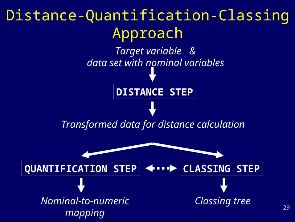
Distance-Quantification-Classing Approach

DISTANCE STEP

QUANTIFICATION STEP CLASSING STEP

Transformed data for distance calculation

Nominal-to-numericmapping

Classing tree

Target variable &data set with nominal variables

10

Example Input to Output

Data:Quality (3): good,ok,bad

Color (6) : blue,green,orange,

purple,red,white

Size (10) : a to j

blue purple green red orange white-0.02 0 -0.54 -0.5 0.55 0.57

Task: Pre-process color based on its patterns across quality and size. Observed Counts COLOR by QUALITY

Good Ok Bad TotalBlue 187 727 546 1460Green 267 538 356 1161Orange 276 411 191 878Purple 155 436 361 952Red 283 307 357 947White 459 366 327 1152Total 1627 2785 2138 6550

11

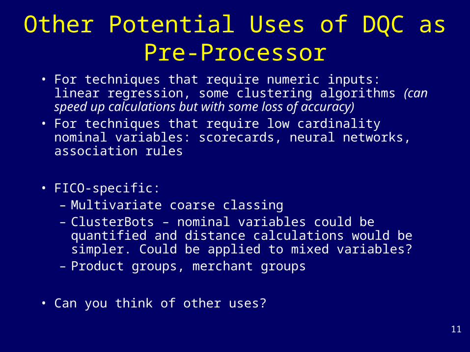
Other Potential Uses of DQC as Pre-Processor

• For techniques that require numeric inputs: linear regression, some clustering algorithms (can speed up calculations but with some loss of accuracy)

• For techniques that require low cardinality nominal variables: scorecards, neural networks, association rules

• FICO-specific:– Multivariate coarse classing– ClusterBots – nominal variables could be quantified and

distance calculations would be simpler. Could be applied to mixed variables?

– Product groups, merchant groups

• Can you think of other uses?

12

Details … Details …

13

• Used for analyzing n-way tables containing some measure of association between rows and columns

• Simple Correspondence Analysis (SCA) – for 2 variables• Multiple Correspondence Analysis (MCA) – for > 2

variables. Uses SCA.• Focused Correspondence Analysis (FCA) – proposed

alternative to MCA when memory is limited. Uses SCA.

• Reinvented as Dual Scaling, Reciprocal Averaging, Homogeneity Analysis, etc.

• Similar to PCA but for nominal variables

Distance Step: Correspondence Analysis

14

Simple Correspondence Analysis – The Basic Idea

Observed Counts COLOR by QUALITY

Good Ok Bad TotalBlue 187 727 546 1460Green 267 538 356 1161Orange 276 411 191 878Purple 155 436 361 952Red 283 307 357 947White 459 366 327 1152Total 1627 2785 2138 6550

Similar profiles

Can we find similar COLORs basedon its association with QUALITY?

Row Percentages

Good Ok BadBlue 13 50 37 100Green 23 46 31 100Orange 31 47 22 100Purple 16 46 38 100Red 30 32 38 100White 40 32 28 100

Calculate 2 statistic (measures thestrength of association between COLOR and QUALITY based onassumption of independence).Any deviation from independencewill increase the 2 value.

15

Identify a few independent dimensions which can reconstruct the 2 value.

(SVD, EigenAnalysis).

Similar row profiles:(blue,purple), …

Similar column profiles:(ok,bad), …

Coordinates for Independent Dimensions

Dim1 Dim2Blue - 0.02 - 0.28Green - 0.54 0.14Orange 0.55 0.10Purple 0 - 0.25Red - 0.50 0.20White 0.57 0.19

Row percentage

matrix

Column percentage

matrix Normalize counts table

Scale the new dimensions such that 2 distances between row points is maximized.

Eigenvalues

Simple Correspondence Analysis – Steps

16

• Coordinates Matrix– Set of independent dimensions– Dimensions ordered by diminishing importance– Total # of independent dimensions = min(r,c)-1– Similar to principal components from PCA

• Eigenvalues– Indicates the importance of each independent

dimension

Simple Correspondence Analysis – The Output

17

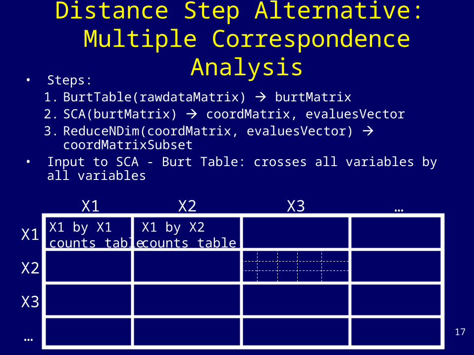
Distance Step Alternative: Multiple Correspondence Analysis

• Steps:1. BurtTable(rawdataMatrix) burtMatrix2. SCA(burtMatrix) coordMatrix, evaluesVector3. ReduceNDim(coordMatrix, evaluesVector)

coordMatrixSubset• Input to SCA - Burt Table: crosses all variables by all variables

X1

X2

X3

…

…X3X2X1X1 by X1counts table

X1 by X2 counts table

18

Multiple Correspondence Analysis

• Features:– For a given variable, determines which values

are similar to each other by comparing value profiles across all other variables

• multivariate

• maximizes usage of information

• memory-intensive

– Simultaneously analyzes of all variables • efficient calculations

19

Reduce Number of Dimensions to Keep

• Reduce the number of independent dimensions to keep for subsequent analysis (due to large # of analysis variables and high cardinality)

eigenvalue

1 2 3 4 5dimension #

20

Distance Step Alternative:Focused Correspondence

Analysis• Proposed alternative to MCA when memory space

is limited• Core idea: instead of comparing value profiles

across all other nominal variables, just compare value profiles across the nominal variables which are most correlated with the target variable

• Input to Simple CA:

targetvariable Xi

…X9X1X3

Xi by X3counts table

Xi by X1 counts table

21

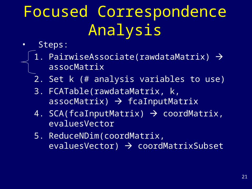
• Steps:

1. PairwiseAssociate(rawdataMatrix) assocMatrix

2. Set k (# analysis variables to use)

3. FCATable(rawdataMatrix, k, assocMatrix) fcaInputMatrix

4. SCA(fcaInputMatrix) coordMatrix, evaluesVector

5. ReduceNDim(coordMatrix, evaluesVector) coordMatrixSubset

Focused Correspondence Analysis

22

FCA: Calculate Pairwise Association

• Used Uncertainty Coefficient U(R|C) to measure strength of nominal association– Bounded [0,1]– U(R|C)=1 value of row variable R can be

known precisely given value of column variable C

• Example: U(R|C) association matrixU(R|C) Quality Color SizeQuality 1.0 0.0287 0.0028Color 0.0173 1.0 0.1234Size 0.0017 0.1267 1.0

23

FCA: Determine top k associated variables for each nominal

variable• Set k >= 2 to ensure use of at least one

analysis variable per target variable

• Cannot use a threshold on the association measure

24

Focused Correspondence Analysis

• Features:– One-at-a-time analysis

• Less/controllable memory usage

• Sub-optimal quantification compared to MCA

– Requires pre-processing step to determine top correlated variables per target variable

• longer run time

25

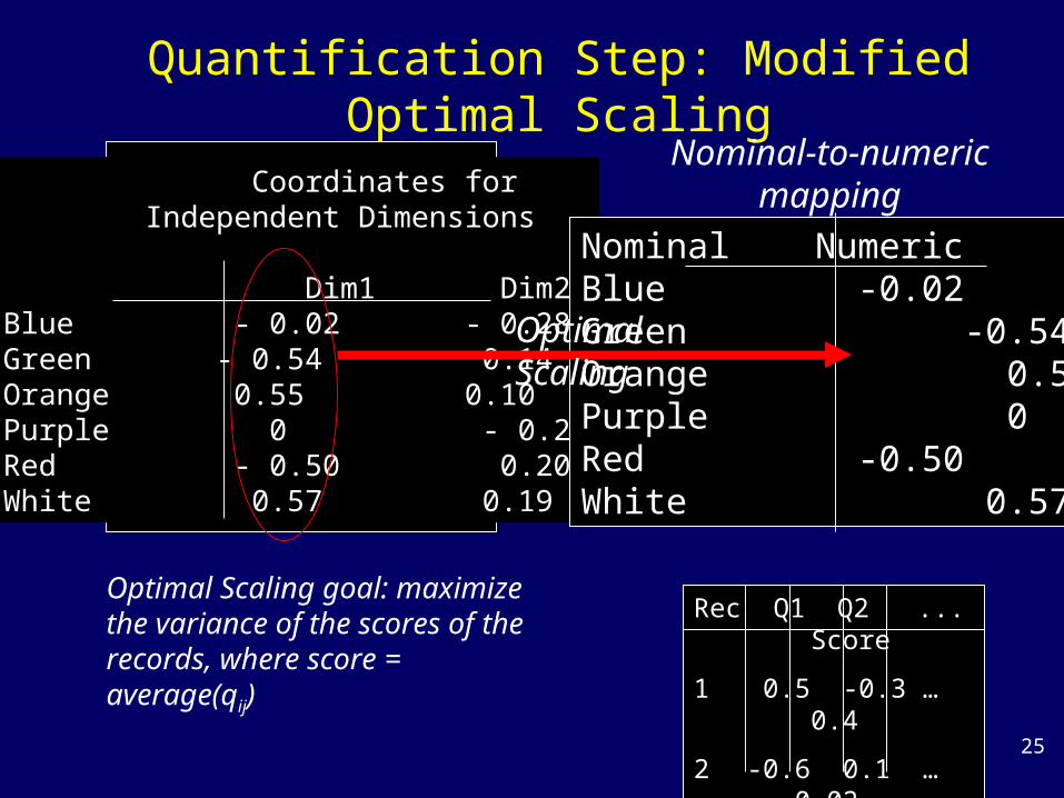
Quantification Step: Modified Optimal Scaling

Coordinates for Independent Dimensions

Dim1 Dim2Blue - 0.02 - 0.28Green - 0.54 0.14Orange 0.55 0.10Purple 0 - 0.25Red - 0.50 0.20White 0.57 0.19

Nominal NumericBlue -0.02Green -0.54Orange 0.55Purple 0Red -0.50White 0.57

Nominal-to-numericmapping

OptimalScaling

Optimal Scaling goal: maximize the variance of the scores of the records, where score = average(qij)

Rec Q1 Q2 ... Score

1 0.5 -0.3 … 0.4

2 -0.6 0.1 … -0.02

…

26

Quantification Step: Modified Optimal Scaling

• Problem with Optimal Scaling: perfect associations between variables are not recreated in the quantified versions

• Modified Optimal Scaling:– Let p = # of eigenvalues = 1.0– If p >= 1 then set

– Else set

p

j

jicoordinateinumeric1

],[][

]1,[][ icoordinateinumeric

27

Cluster Analysisweighted by counts

blue purple green red orange white

[from FCA]

Classing Step: Hierarchical Cluster Analysis

Coordinates for Independent Dimensions

Dim1 Dim2 CountsBlue - 0.02 - 0.28 1460Green - 0.54 0.14 1161Orange 0.55 0.10 878Purple 0 - 0.25 952Red - 0.50 0.20 947White 0.57 0.19 1152

28

Loss of Information due to Classing

blue purple green red orange white Info loss

100

50

0

1. Determine variable V with highest association with target X.2. Create X by V counts table.3. Calculate total table measure of association (eg, U(X|V)).4. Starting from bottom of tree, for every pair of nodes merged,

calculate cumulative information loss:

)(

))()((*100

fullTableA

ngafterMergiAfullTableAInfoLoss

Observed Counts COLOR by SIZEU(R|C) = 0.1234

a b … j TotalBlue 0 8 … 1460Green 0 2 … 1161Orange 7 49 … 878Purple 0 5 … 952Red 0 0 … 947White 6 70 … 1152Total 13 134 … 6550

29

Distance-Quantification-Classing Approach

DISTANCE STEP

QUANTIFICATION STEP CLASSING STEP

Transformed data for distance calculation

Nominal-to-numericmapping

Classing tree

Target variable &data set with nominal variables

30

Does this approach work?

31

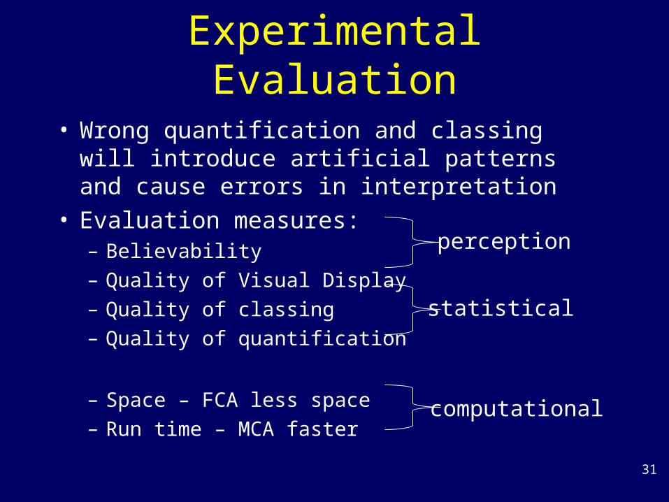
Experimental Evaluation

• Wrong quantification and classing will introduce artificial patterns and cause errors in interpretation

• Evaluation measures:– Believability

– Quality of Visual Display

– Quality of classing

– Quality of quantification

– Space – FCA less space

– Run time – MCA faster

perception

computational

statistical

32

Test Data Sets

33

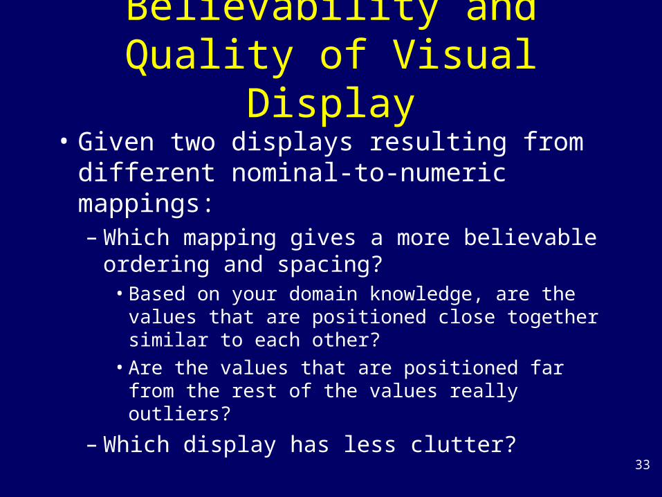
Believability and Quality of Visual Display

• Given two displays resulting from different nominal-to-numeric mappings:– Which mapping gives a more believable

ordering and spacing?• Based on your domain knowledge, are the values

that are positioned close together similar to each other?

• Are the values that are positioned far from the rest of the values really outliers?

– Which display has less clutter?

34

Automobile Data: Alphabetical

35

Automobile Data: MCA

Are thesepatterns believable?

36

Automobile Data: FCA

Are thesepatterns believable?

37

PERF Data: Alphabetical

Region-Country:1-many

Country-Product:many-many

Are these associationspreserved andrevealed?

38

PERF Data: FCA

Region-Country:1-many

Country-Product:many-many

Are these associationspreserved andrevealed?

39

Quality of Classing• Classing A is better than classing B if,

given a classing tree, the rate of information loss with each merging is slower

Information lossdue to classingfor one variable

[The lower the line,the slower the info loss,the better the classing.]

Calculatedifferencebetween the lines.

40

Which classing is better … depends on dataset

Distribution ofdifferencebetween the lines.

41

Quality of Quantification

• A quantification is good if …1. If data points that are close together in

nominal space are also close together in numeric space

2. If two variables are highly associated with each other, then their quantified versions should also have high correlation.

42

MCA gives better quantification

Correlation between

MCA and FCA scales[how close are FCA

scales to MCA scales]

AverageSquaredCorrelation[higher value = better quantification]

43

Had enough yet?

44

Going back to Multivariate Coarse Classing

• Other issues:– Missing values– Mixed or numeric variables as analysis

variables– Nominal values with small counts– Robustness of quantification and classing

45

Can you think of other uses of DQC at FICO?

• For techniques that require numeric inputs: linear regression, some clustering algorithms (can speed up calculations but with some loss of accuracy)

• For techniques that require low cardinality nominal variables: scorecards, neural networks, association rules

• FICO-specific:– Multivariate coarse classing– ClusterBots – nominal variables could be quantified

and distance calculations would be simpler. Could be applied to mixed variables?

– Product groups, merchant groups– ???????

46

Implementation

• SAS version exists– PROC CORRESP, PROC CLUSTER, PROC

FREQ

• C++ version in development

47

Summary• DQC is a general-purpose approach for pre-processing

nominal variables for data analysis techniques requiring numeric variables or low cardinality nominal variables

• DQC – multivariate, data-driven, scalable, distance-preserving, association-preserving

• FCA is a viable alternative to MCA when memory space is limited

• Quality of classing and quantification – depends on strength of associations within the data set.– is in the eye of the user

48

Yippee, it’s over!

Original InfoVis2003 paper: Mapping Nominal Values to Numbers for Effective Visualization.http://davis.wpi.edu/~xmdv/documents.html

XmdvTool Homepage: http://davis.wpi.edu/~xmdv

xmdv@cs.wpi.eduCode is free for research and education.

49

References• [Gre93] GREENACRE, M.J., 1993, Correspondence Analysis in

Practice, London :Academic Press• [Gre84] Greenacre, M. (1984), Theory and Applications of

Correspondence Analysis, London: Academic Press• [Sta] StatSoft Inc. Correspondence Analysis.

http://www.statsoftinc.com/textbook/stcoran.html• [Fri99] Friendly, Michael. 1999. "visualizing Categorical Cata." In

Sirken, Monroe G. et. al. (eds). Cognition and Survey Research. New York: John Wiley & Sons.

• [Kei97] Keim D. A.: Visual Techniques for Exploring Databases, Invited Tutorial, Int. Conference on Knowledge Discovery in Databases (KDD'97), Newport Beach, CA, 1997.

• [Hua97b] Zhexue Huang. A Fast Clustering Algorithm to Cluster Very Large Categorical Data Sets in Data Mining (1997)

• SAS Manuals (PROC CORRESP, PROC CLUSTER, PROC FREQ)

50

What input tables can SCA accept?

• In general, SCA can use as input any table that has the properties:

1. The table must use the same physical units or measurements, and

2. The values in the table must be non-negative.

The FCA input table satisfies these properties.

51

Uncertainty Coefficient U(R|C)

r

iijjj

c

jjC

c

jijii

r

iiR

ij

r

iij

c

jijRC

R

RCCR

ppppH

ppppH

pppH

HHHH

jCiRP

CRU

11

11

1 1

),log(

),log(

],[ ,)log(

)|(

Source: SAS Proc Freq

52

Average Squared Correlation

• Given the raw data matrix R=[rij], where the columns represent the variables. Create new matrix Q=[qij] where qij.=quantified version of rij.. Let Qj=jth column of Q.

• For each record i, calculate scorei=average(j qij )

• For each variable j, calculate corrj=correlation(Qi,score)

• Calculate average of the squared correlation.

Source: [Gre93]

Rec Q1 Q2 ... Score

1 0.5 -0.3 … 0.4

2 -0.6 0.1 … -0.02

…

Pair Sqr(Correlation)Q1,score 0.36Q2,score 0.49…

average=___