arX

iv:1

302.

1489

v1 [

cs.IT

] 6

Feb

201

31

Multi-rate Sub-Nyquist Spectrum Sensing in

Cognitive Radios

Hongjian Sun,Member, IEEE,A. Nallanathan∗, Senior Member, IEEE,

Jing Jiang,Member, IEEE,and Cheng-Xiang Wang,Senior Member, IEEE

Abstract

Wideband spectrum sensing is becoming increasingly important to cognitive radio (CR) systems

for exploiting spectral opportunities. This paper introduces a novel multi-rate sub-Nyquist spectrum

sensing (MS3) system that implements cooperative wideband spectrum sensing in a CR network. MS3

can detect the wideband spectrum using partial measurements without reconstructing the full frequency

spectrum. Sub-Nyquist sampling rates are adopted in sampling channels for wrapping the frequency

spectrum onto itself. This significantly reduces sensing requirements of CR. The effects of sub-Nyquist

sampling are considered, and the performance of multi-channel sub-Nyquist samplings is analyzed. To

improve its detection performance, sub-Nyquist sampling rates are chosen to be different such that the

numbers of samples are consecutive prime numbers. Furthermore, when the received signals at CRs are

faded or shadowed, the performance of MS3 is analytically evaluated. Numerical results show that the

proposed system can significantly enhance the wideband spectrum sensing performance while requiring

low computational and implementation complexities.

Index Terms

Cognitive radio, Spectrum sensing, Sub-Nyquist sampling,Rayleigh distribution, Log-normal dis-

tribution.

H. Sun and A. Nallanathan∗ are with the Department of Electronic Engineering, King’s College London, London, WC2R2LS, UK. (Email: hongjian.sun@kcl.ac.uk; nallanathan@ieee.org)

J. Jiang is with Center for Communication Systems Research,University of Surrey, Guildford, GU2 7XH, UK. (Email:jing.jiang@surrey.ac.uk)

C.-X. Wang is with Joint Research Institute for Signal and Image Processing, School of Engineering & Physical Sciences,Heriot-Watt University, Edinburgh, EH14 4AS, UK. (Email: Cheng-Xiang.Wang@hw.ac.uk)

March 4, 2018 DRAFT

2

I. INTRODUCTION

The radio frequency (RF) spectrum is a scarce natural resource, currently regulated by gov-

ernment agencies. Under the current policy, the primary user (PU) of a particular spectral band

has exclusive rights to the licensed spectrum. With the proliferation of wireless services, the

demands for the RF spectrum are continually increasing. On the other hand, it has been reported

that localized temporal and geographic spectrum utilization efficiency is extremely low. For

example, it has been reported that the maximal occupancy of the spectrum between 30 MHz

and 3 GHz is only13.1% and its average occupancy is5.2% in New York City [1]. The spectral

under-utilization can be addressed by allowing secondary users to access a licensed band when

the PU is absent. Cognitive radio (CR) has become one promising solution for realizing this

goal [2], [3].

A crucial requirement of CRs is that they must rapidly fill spectral holes without causing

harmful interference to the PUs. This ability is dependent upon spectrum sensing, which is

considered as one of the most critical components in a CR system. In a multipath or shadow

fading environment, the signal-to-noise ratio (SNR) of theprimary signal as received at CRs

can be severely degraded, which will not only lead to unreliable spectrum sensing results, but

will also reduce the capacity of the CR network due to the decreased data transmission time per

frame. In such a scenario, cooperative spectrum sensing could increase the reliability of spectrum

sensing by exploiting spatial diversity. In our previous work [4], [5], centralized cooperative

spectrum sensing frameworks have been developed for improving the reliability of spectrum

sensing. However, these studies only considered narrowband spectrum sensing techniques, the

extension to wideband cooperative spectrum sensing requires yet a different approach.

To exploit more spectral opportunities over a large range offrequencies (e.g., 10 kHz∼ 10

GHz), a CR system needs some essential components, i.e., wideband antenna, wideband RF

front end, and high speed analog-to-digital converter (ADC). Yoon et al. [6] have shown that

the −10 dB bandwidth of the newly designed antenna can be 14.2 GHz. Hao and Hong [7]

designed a compact highly selective wideband bandpass filter with a bandwidth of 13.2 GHz.

In [8], Bevilacqua and Niknejad designed a wideband CMOS low-noise amplifier with

March 4, 2018 DRAFT

3

the bandwidth of approximately 10 GHz. In contrast, the development of ADC technology

is relatively behind. To the best of our knowledge, when we require an ADC to have a high

resolution and a reasonable power consumption, the achievable sampling rate of the current ADC

is 3.6 Gsps [9]. Obviously, ADC becomes a bottleneck in such awideband system. Even if there

exists ADC with more than 20 Gsps sampling rate, the real-time digital signal processing of 20

Gb/s of data could be very expensive.

In previous work, Quanet al. [10], [11] proposed a multiband joint detection (MJD) approach

that can sense the primary signal over a wide frequency range. It has been shown that MJD

has superior performance for multiband spectrum sensing. In [12], Tian and Giannakis studied

a wavelet detection approach, which could adapt parametersto a dynamic wideband spectrum.

Furthermore, they cleverly introduced compressed sensing(CS) theory to implement wideband

spectrum sensing by using sub-Nyquist sampling techniquesin the classic paper [13]. Later on,

the CS-based approach has attracted many talented-researchers’ attention in [14]–[24] owning

to its advantage of using fewer samples closer to the information rate, rather than the inverse

of the bandwidth, to perform wideband spectrum sensing. In [14], Tian et al. studied cyclic

spectrum sensing techniques with high robustness against sampling rate reduction and noise

uncertainty. In [15], Zenget al. proposed a distributed CS-based spectrum sensing approach

for cooperative multihop CR networks. In our previous work [25], [26], to save system energy,

adaptive CS-based spectrum sensing approaches were proposed that could find the best spectral

recovery with high confidence. Unfortunately, using CS-based approaches, the spectral recovery

may cause high computational complexity, leading to a high spectrum sensing overhead due to

the restricted computational resources in CRs.

In this paper, we introduce a multi-rate sub-Nyquist spectrum sensing (MS3) approach for

cooperative wideband spectrum sensing in a CR network. Because the spectral occupancy is

low, sub-Nyquist sampling is induced in each sampling channel to wrap the sparse spectrum

occupancy map onto itself. The sensing requirements are therefore significantly reduced. We

then analyze the effects caused by sub-Nyquist sampling, and represent the test statistic using a

reduced data set obtained from multi-channel sub-Nyquist sampling. Furthermore, we propose to

March 4, 2018 DRAFT

4

use different sampling rates in different sampling channels for improving the spectrum sensing

performance. Specifically, in the same observation time, the number of samples in multiple sam-

pling channels are chosen as different consecutive prime numbers. In addition, the performance

of MS3 for combining faded or shadowed signals is analyzed, and theclosed-form bounds for

the average probabilities of false alarm and detection are derived. The key advantage of MS3 is

that the wideband spectrum can be detected directly from a few sub-Nyquist samples without

spectral recovery. Compared to the existing spectrum sensing methods, MS3 can achieve better

wideband spectrum sensing performance with a relatively lower implementation complexity.

The rest of the paper is organized as follows. Section II introduces the signal model. In Section

III, we propose the wideband spectrum sensing approach, i.e., MS3. The performance analysis of

MS3 for combining faded signals is given in Section IV. Section Vpresents simulation results,

and conclusions are given in Section VI.

II. PRELIMINARY

Consider that all CRs keep quiet during the spectrum sensinginterval as enforced by protocols,

e.g., at the medium access control (MAC) layer [10]. Therefore, the observed spectral energy

arises only from PUs and background noise. The bandwidth of the signal as received at CRs

is W (Hertz). Over an observation timeT , if the sampling ratef (f ≥ 2W ) is adopted to

sample the received signal, a sequence of Nyquist samples will be obtained with the length of

JN= fT . This sequence is then divided intoJ equal-length segments whereN denotes the

number of Nyquist samples per segment (bothJ andN are chosen to be natural numbers). If

we usexc,i(t) (t ∈ [0, T ]) to represent the continuous-time signal received at CRi, after Nyquist

sampling, the sampled signal can be denoted byxi[n] = xc,i(n/f), n = 0, 1, · · · , JN − 1. At

CR i, the sampled signal of segmentj (j ∈ [1, J ]) can be written as

xi,j [n] =

xc,i(n/f), n = (j − 1)N, (j − 1)N + 1, · · · , jN − 1

0, Otherwise.(1)

March 4, 2018 DRAFT

5

The discrete Fourier transform (DFT) spectrum of the sampled signal of segmentj is given by

Xi,j[k] =

N−1∑

n=0

xi,j [n]e−2πkn/N , k = 0, 1, · · · , N − 1 (2)

where =√−1. We model spectrum sensing on a frequency bink as a binary hypothesis test,

i.e., H0,k (absence of PUs) andH1,k (presence of PUs) [11]:

Xi,j[k] =

Zi,j[k], H0,k

Hi,j[k]Si,j[k] + Zi,j[k], H1,k or k ∈ Ωi(3)

whereZi,j[k] is complex additive white Gaussian noise (AWGN) with zero mean and variance

δ2i,k, i.e.,Zi,j[k] ∼ CN (0, δ2i,k), Hi,j[k] denotes the discrete frequency response between the PU

and CRi, Si,j[k] is assumed to be a deterministic signal sent by the PU on the frequency bink,

andΩi denotes the spectral support such thatΩi = k|PU presents atXi,j[k]. For simplicity,

in the rest of the paper, we assume that the noise variance of the DFT spectrum is normalized

to be 1. The observation timeT is chosen to be smaller than the channel coherence time so that

the magnitude ofHi,j[k] remains constant withinT for one CR, i.e., constant|Hi,j[k]| regarding

the segment numberj.

Because an energy detector does not require any prior information about the transmitted

primary signal while having lower complexity than other spectrum sensing approaches [27],

we consider the energy detection approach in this paper. Thereceived signal energy can be

calculated as

Ei[k] =

J∑

j=1

|Xi,j[k]|2 , k = 0, 1, · · · , N − 1. (4)

The decision rule for energy detection approach is then given by

H1,k

Ei[k] R λk, k = 0, 1, · · · , N − 1 (5)

H0,k

whereλk is the detection threshold for the frequency bink. Here, it is noteworthy to empha-

size that, after Fourier transform, the energy detection isdone on each frequency bin in the

frequency domain. Thus, the noise in high frequencies should not affect the energy detection in

low frequencies, and vice versa. The benefit of frequency-domain energy detection is that the

March 4, 2018 DRAFT

6

detection performance depends on the SNRon a single frequency bin, regardless of the noise in

the other frequencies(e.g., high frequency noise due to wideband sensing). To be specific, the

signal energy on frequency bink can be modeled by [27]

Ei[k] ∼

χ22J , H0,k

χ22J(2γi[k]), H1,k

(6)

whereγi[k]=

E(|Hi[k]Si[k]|2)δ2i,k

denotes the SNR on the frequency bink at CRi, χ22J denotes central

chi-square distribution, andχ22J(2γi[k]) denotes non-central chi-square distribution. Both of these

distributions have2J degrees of freedom and2γi[k] denotes a non-centrality parameter. Here,

the noise has varianceδ2i,k, measured bandwidthfN

, and noise temperatureTn =δ2i,kN

fKBwhereKB

denotes the Boltzmann constant. The probabilities of falsealarm and detection are given by [27]

Pf,i,k=Pr(Ei[k] > λk|H0,k) =Γ(J, λk

2)

Γ(J)(7)

Pd,i,k=Pr(Ei[k] > λk|H1,k) = QJ

(√2γi[k],

√λk

)(8)

whereΓ(a) denotes the gamma function,Γ(a, x) denotes the upper incomplete gamma function,

andQu(a, x) is the generalized Marcum Q-function defined byQu(a, x) =1

au−1

∫∞xtue−

a2+t2

2 Iu−1(at)dt

in which Iv(a) is thev-th order modified Bessel function of the first kind.

III. MULTI -RATE SUB-NYQUIST SPECTRUM SENSING

It is difficult to realize wideband spectrum sensing, because it requires a high speed ADC for

Nyquist rate sampling. We will now present an MS3 system using multiple low-rate samplers to

implement wideband spectrum sensing in a CR network.

A. System Description

Consider that there arev synchronized CRs collaborating for wideband spectrum sensing, and

the fusion center (FC) is one of the CRs which has either greater computational resources or

longer battery life than other CRs. Due to low spectral occupancy [13], the received signals at

CRs are often sparse in the frequency domain. Here, we assumethat the Nyquist DFT spectrum,−−→Xi,j ∈ CN , is s-sparse (s≪ N), which means that only the largests out ofN components cannot

March 4, 2018 DRAFT

7

be ignored. The spectral sparsity level, i.e.,s, can be obtained from either sparsity estimation [16]

or system initialization (e.g., by long term spectral measurements). As shown in Fig. 1, MS3

consists of several CRs, each of which has one wideband filter, one low-rate sampler, and a fast

Fourier transform (FFT) device. The wideband filters are setto have bandwidth ofW . MS3 can

be described as follows:

1) The FC allocates different sub-Nyquist sampling rates todifferent CRs.

2) CRs perform sub-Nyquist samplings in the observation time T .

3) The sub-Nyquist DFT spectrum is calculated by using sub-Nyquist samples and FFT

device1.

4) The signal energy vectors are formed by using the sub-Nyquist DFT spectrum.

5) The CRs transmit these signal energy vectors to the FC by using a dedicated common

control channel in a band licensed to the CR network [28].

6) The received data from all CRs is fused in the FC to form a test statistic.

7) The FC chooses the detection threshold and performs binary hypothesis tests.

8) The FC shares the detection results with all CRs.

B. Sub-Nyquist Sampling and Data Combining

At CR i, we use sub-Nyquist ratefi (fi < 2W ≤ f ) to sample the continuous-time signal

xc,i(t). The sampled signal can be denoted byyi[n] = xc,i(n/fi), n = 0, 1, · · · , JMi − 1 where

JMi = fiT andMi is assumed to be a natural number. The sampled signal is then divided into

J equal-length segments. The segmentj (j ∈ [1, J ]) can be written as

yi,j[n] =

xc,i(n/fi), n = (j − 1)Mi, (j − 1)Mi + 1, · · · , jMi − 1

0, Otherwise.(9)

The DFT spectrum of the sampled signal of segmentj (j ∈ [1, J ]) can be given by

Yi,j[m] =

Mi−1∑

n=0

yi,j[n]e−2πmn/Mi , m = 0, 1, · · · ,Mi − 1 (10)

1Jointly considering wideband spectrum sensing and spectrum reuse in CRs, we use FFT devices for distinguishing differentfrequencies in order to reuse some un-occupied frequencies. Here, the use of FFT will cause additional complexity ofO(M logM) and memory storage increment, ifM denotes the number of FFT points.

March 4, 2018 DRAFT

8

With the aid of Poisson summation formula [29], the DFT spectrum of sub-Nyquist samples can

be represented by the DFT spectrum of Nyquist samples (as proved in Appendix A):

Yi,j[m] =Mi

N

∞∑

l=−∞Xi,j[m+ lMi], m = 0, 1, · · · ,Mi − 1. (11)

According to (3) and (11), the spectral support of the sub-Nyquist spectrum−→Yi,j can be given

by

Ωs,i = m|m = |k| mod (Mi), k ∈ Ωi. (12)

One risk caused by sub-Nyquist sampling is the signal overlap in Yi,j[m]. However, when we

choose parameters inJN = fT such thatN ≫ s and let the sub-Nyquist sampling rate satisfy

Mi ∼ O(√N), the probability of signal overlap is very small (as proved in Appendix B). In

such a scenario, we concentrate on considering two cases: nosignal onm and one signal onm.

In the latter case, only a singlel is active in (11), and the other terms in the summation of (11)

can be modeled as noise by using (3). Thus, the following equation holds from (3) and (11):

Yi,j[m] =Mi

NXi,j[m+ lMi] +

Mi

N

∑

ν 6=lZi,j[m+ νMi], m+ lMi ∈ Ωi (13)

where l is an unknown integer within[0, N/Mi − 1]. Furthermore, using (3) and (13), we can

model the DFT spectrum of sub-Nyquist samples by

√N

Mi

Yi,j

[|k| mod (Mi)

]∼

CN(0, δ2s,i,k

), k /∈ Ωi

CN(√

Mi

NHi,j[k]Si,j[k], δ

2s,i,k

), k ∈ Ωi

(14)

whereδ2s,i,k is the noise variance of sub-Nyquist DFT spectrum, and can begiven by using (11)

δ2s,i,k =

⌈N

Mi

⌉

︸ ︷︷ ︸No. of sums

(Mi

N

√N

Mi︸ ︷︷ ︸Scaling of Yi,j

)2

δ2i,k ≈ δ2i,k (15)

where⌈ NMi

⌉ (the smallest integer not less thanNMi

) denotes the number of summations in (11).

The signal energy of sub-Nyquist DFT spectrum in each CR nodeis then calculated by

Es,i[m] =J∑

j=1

|Yi,j[m]|2 , m = 0, 1, · · · ,Mi − 1. (16)

March 4, 2018 DRAFT

9

which can be modeled by using (14) and (16) as

N

MiEs,i

[|k| mod (Mi)

]∼

χ22J , k /∈ Ωi

χ22J

(2Mi

Nγi[k]

), k ∈ Ωi.

(17)

We note that, due to the sub-Nyquist sampling, the noise willbe folded from the whole

bandwidth onto all signals of interest as shown in (13). As a result, comparing (17) with

(6), we find that the received SNR in the sub-Nyquist samplingchannel i will degrade from

γi to Mi

Nγi. This SNR degradation depends on the ratio between the number of samples at

the sub-Nyquist rate and the number of samples at the Nyquistrate (i.e., Mi

N).

In MS3, the signal energy vectors at CRs will then be collected at the FC. Finally, we form

a test statistic by

Es[k] =v∑

i=1

N

Mi

Es,i[|k| mod (Mi)], k = 0, 1, · · · , N − 1. (18)

In Fig. 2, we give an illustration of the above test statisticfor a practical ASTC DTV signal.

To test whether the PU is present or not, we adopt the following decision rule:

H1,k

Es[k] R λk, k = 0, 1, · · · , N − 1. (19)

H0,k

Let ΩA,i denote a set of aliased frequencies (i.e., false frequencies appear as mirror images of

the original frequencies around the sub-Nyquist sampling frequency), andΩU,i represent a set

of unaffected/unoccupied frequencies:

ΩA,i=k∣∣∣m = |k| mod (Mi), m ∈ Ωs,i, k /∈ Ωi

(20)

ΩU,i=k∣∣∣m = |k| mod (Mi), m /∈ Ωs,i, k /∈ Ωi

. (21)

Using (17), we can model the test statistic of (18) as

Es[k] ∼

χ22Jv, k ∈ ΩU

χ22Jv

(2N

|Υ|=p∑i∈Υ

Miγi[k]

), k ∈ ΩA

χ22Jv

(2N

v∑i=1

Miγi[k]

), k ∈ Ω

(22)

March 4, 2018 DRAFT

10

whereΩU= ∩vi=1ΩU,i, ΩA

= ∪vi=1ΩA,i, Ω

= ∩vi=1Ωi, Υ

= i|m = |k| mod (Mi), m ∈ Ωs,i, k /∈ Ωi

denotes the set of CRs who have aliased frequency on the frequency bink, and|Υ| = p denotes

the cardinality of the setΥ (equivalently the number of CRs that have aliased frequencies on

the frequency bink).

In (22), k ∈ ΩU and k ∈ ΩA are two extreme cases under the hypothesisH0,k. The former

case denotes there is no aliased frequency on the frequency bin k, while the latter case represents

there are maximum number of aliased frequencies (i.e.,p) on the frequency bink. Thus, the

former one is the best case while the latter one is the worst case for signal detection under the

hypothesisH0,k. The probability of false alarm on the frequency bink can therefore be bounded

by using (22)

Γ(Jv, λk2)

Γ(Jv)≤ Pf,k ≤ QJv

√√√√ 2

N

|Υ|=p∑

i∈ΥMiγi[k],

√λk

. (23)

We note that the problem of minimizing the probability of false alarm can be transformed to

minimize the parameterp, which depends on several factors, e.g., the sampling ratesof CRs.

Using the same sub-Nyquist sampling rates in MS3 is not recommended as it could lead to

p = v, resulting in the maximum of the probability of false alarm.As we will see in the

following subsection, the parameterp can be minimized by using different sampling rates at

CRs.

C. Multi-rate Sub-Nyquist Spectrum Sensing

To improve the detection performance of sub-Nyquist sampling system in the preceding

subsection, we should analyze the influence of sampling rates. Firstly, we consider the case

of spectral sparsity levels = 1, which means that only one frequency bink1 ∈ Ω is occupied

by the PU.

Lemma 1: If the numbers of samples in multiple CRs, i.e.,M1,M2, ...,Mv, are different

primes, and meet the requirement of

MiMj > N, ∀ i 6= j ∈ [1, v] (24)

March 4, 2018 DRAFT

11

then two or more CRs cannot have mirrored frequencies in the same frequency bin.

The proof of Lemma 1 is given in Appendix C.

Secondly, considering the spectral sparsity levels ≥ 2, we find that, if the conditions in

Lemma 1 are satisfied, the parameterp in (22) is bounded bys. It is because only one CR can

map the original frequency binkj ∈ Ωi to the aliased frequency inΩA , and the cardinality of the

spectral supportΩi is s. Therefore, we obtain the detection performance of MS3 as Theorem 1.

Theorem 1:In MS3, if the numbers of samples in multiple CRs, i.e.,M1,M2, · · · ,Mv, are

different consecutive primes, and meet the requirement ofMiMj > N, ∀ i 6= j ∈ [1, v], using

the decision rule of (19) the probabilities of false alarm and detection have the following bounds:

Γ(Jv, λk2)

Γ(Jv)≤ Pf,k ≤ QJv

√√√√ 2

N

|Υ|=s∑

i∈ΥMiγi[k],

√λk

(25)

Pd,k≥ QJv

√√√√ 2

N

v∑

i=1

Miγi[k],√λk

. (26)

Proof: Using (23) and the bound|Υ| = p ≤ s, (25) follows. Furthermore, when the energy

of one spectral component inΩ maps to another spectral component inΩ, the probability of

detection will increase. Thus, the inequality of (26) holds.

Remark 1: It can be seen from Theorem 1 that the sampling rates in MS3 can be much lower

than the Nyquist rate because ofMi ∼ O(√N). By (25) we note that the probability of false

alarm increases when the spectral sparsitys increases. In addition, the higher average sampling

rate will lead to better detection performance. This is because the probability of signal overlap in

the aliased spectrum can be reduced with a largerMi in each sampling channel as our discussions

in Section III-B. By (25) and (26), we can see that using more sampling channels (i.e.,v), the

detection performance can be improved. It should be emphasized that there is no closed-form

expression for the probabilities in Theorem 1. This is because the number of CRs that have

aliased frequencies on the frequency bink cannot be predicted. Moreover, we note that the

upper and lower bounds in Theorem 1 can be easily computed because the Marcum-Q function

can be efficiently computed using power series expansions [30]. Under the Neyman-Pearson

March 4, 2018 DRAFT

12

criterion, we should design a test with the constraint ofPf,k ≤ α. In such a scenario, we must

let the upper bound of (25) to beα and solve the detection thresholdλk from the inverse of the

Marcum-Q function. It has been shown in [31] that the detection threshold can be calculated

with low computational complexity. In addition, to calculate the detection threshold, the noise

power is required to be known at the FC.

IV. COMBINATION OF FADED SIGNALS

As shown in Section III, the combining procedure in the FC is to sum up all non-faded signals

at CRs and make final decisions. In this section, we investigate the combination of faded signals

at CRs using the same approach as shown in (18). We assume thatthe received primary signals

at different CRs are independent and identically distributed (i.i.d.), and are faded subject to either

Rayleigh or log-normal distribution.

Solving the distribution of the sum of weighted independentrandom variables in (18) is not

trivial. Hence, we use the sum of uniformly weighted random variables to approximate the sum

of different weighted random variables in Theorem 1:

2v∑i=1

Miγi

N≃ 2M

N

v∑

i=1

γi = ψγv,

2|Υ|=s∑i∈Υ

Miγi

N≃ 2M

N

|Υ|=s∑

i∈Υγi = ψγs (27)

whereM is the averageMi over multiple CRs,ψ= 2M

N, γv

=∑v

i=1 γi, andγs=∑|Υ|=s

i∈Υ γi. We

note that the above approximation accuracy mainly depends on |M−Mi|N

, where smaller|M−Mi|N

corresponds to more accurate approximation. SinceM1,M2, ...,Mv are chosen to bev different

consecutive prime numbers and the distance between primes could be very small compared to

N , the parameter|M−Mi|N

will approach to zero asN increases. Thus, the above approximation

has little impact on the final result.

March 4, 2018 DRAFT

13

A. Rayleigh Distribution

If the magnitudes of received signals at different CRs follow Rayleigh distribution, then the

SNRs will follow exponential distribution. Hence,γv andγs follow Gamma distributions:

f(γv) =γv−1

v

γvΓ(v)e−

γvγ , γv ≥ 0, f(γs) =

γs−1s

γsΓ(s)e−

γsγ , γs ≥ 0 (28)

where γ = E( |HS|2

δ2) denotes average SNR over multiple CRs, andf(·) denotes a generic

probability density function (PDF) of its argument.

The average probabilities of false alarm and detection for MS3 are often solved by averaging

Pf,k in (25) andPd,k in (26) over all possible SNRs, respectively.

Theorem 2:If the magnitudes of received signals at different CRs follow Rayleigh distribution,

the average probabilities of false alarm (Pf,k) and detection (Pd,k) in MS3 will have the following

bounds

Γ(Jv, λk2)

Γ(Jv)≤ Pf,k ≤ Θ(s, Jv, ψ, γ[k], λk) (29)

Pd,k≥ Θ(v, Jv, ψ, γ[k], λk) (30)

whereΘ(x, Jv, ψ, γ, λ) is defined as

Θ =

(1 +

ψγ

2

)−x ∞∑

n=0

Cnn+x−1

(ψγ

ψγ + 2

)n Γ(n + Jv, λ

2

)

Γ (n+ Jv)(31)

in which Cba denotes the binomial coefficient, i.e., Cba =b!

a!(b−a)! .

The proof of Theorem 2 is given in Appendix D.

Remark 2: From Theorem 2, we can see that0 ≤ Θ ≤ 1, because the termΓ(a,b)Γ(a)

∈ [0, 1] and

the remaining terms can be simplified to 1. In addition, it canbe proved thatΘ is a monotonically

increasing function with respect toψ, γ, andx. Therefore, both probabilities will either increase

or remain the same when the average sampling rate and the average SNR increase, more sampling

channels will lead to a higher probability of detection, andthe average probability of false alarm

can be reduced with smallers.

Remark 3: Because (31) contains infinite sums, its computational complexity is directly related

to the number of computed terms that are required in order to obtain a specific accuracy. As the

March 4, 2018 DRAFT

14

number of computed terms, i.e.,P , varies, the truncation error can be written as

TΘ(P ) =

(1 +

ψγ

2

)−x ∞∑

n=P

Cnn+x−1

(ψγ

ψγ + 2

)n Γ(n+ Jv, λ

2

)

Γ (n+ Jv)(32)

≤(1 +

ψγ

2

)−x ∞∑

n=P

Cnn+x−1

(ψγ

ψγ + 2

)n(33)

= 1−(1 +

ψγ

2

)−x P−1∑

n=0

Cnn+x−1

(ψγ

ψγ + 2

)n(34)

where the inequality of (33) holds becauseΓ(n,λ

2)

Γ(n)≤ 1, and (34) is obtained by using the binomial

expansion. It can be shown that (31) converges very quickly.For example, in order to achieve

double-precision accuracy, onlyP = 30 ∼ 40 calculated terms are required; therefore the bounds

are tractable. To solve for the detection thresholdλk, we could use the lower bound onPf,k in

(30). This is because the lower bound can approximatePf,k very well as analyzed in Appendix D

and also verified by Fig. 3.

B. Log-normal Distribution

The strength of the transmitted primary signal is also affected by shadowing from buildings,

hills, and other objects. A common model is that the receivedpower fluctuates with a log-normal

distribution. In such a scenario, the PDF of the SNR at CRi, i.e., f(γi), is given by

f(γi) =ξ√

2πσiγiexp

(−(10 log10(γi)− γi)

2

2σ2i

), γi > 0 (35)

whereξ = 10/ ln(10), andσi (dB) denotes the standard deviation of10 log10 γi at CR i. Note

that the PDF in (35) can be closely approximated by a Wald distribution [27], [32]:

f(γi) =

√ηi2πγ−3/2i exp

(−ηi(γi − θi)

2

2θ2i γi

), γi > 0 (36)

whereθi = E(γi) denotes the expectation ofγi, andηi is the shape parameter for CRi. Via the

method of moments, the parametersηi, θi andγi, σi are related as follows:

θi = exp

(γiξ+

σ2i

2ξ2

), ηi =

θi

exp(σ2iξ2)− 1

. (37)

In the proposed system, the conditionηiθ2i

= E(γi)Var(γi)

= b (constant) can be satisfied. Thus,γs

March 4, 2018 DRAFT

15

andγv will also follow the Wald distribution [33]. The PDFs ofγs andγv are given by

f(γs) =

√sη

2πγ−3/2

s exp

(−η(γs − sθ)2

2sθ2γs

), γs > 0 (38)

f(γv) =

√vη

2πγ−3/2

v exp

(−η(γv − vθ)2

2vθ2γv

), γv > 0 (39)

whereη andθ denote the averages ofηi andθi, respectively.

Theorem 3:If the magnitudes of received signals at different CRs follow log-normal distribu-

tion, the average probabilities of false alarm (Pf,k) and detection (Pd,k) in MS3 will be bounded

as

Γ(Jv, λk2)

Γ(Jv)≤ Pf,k ≤ Λ(s, Jv, ψ, λk, θ[k], η[k]) (40)

Pd,k ≥ Λ(v, Jv, ψ, λk, θ[k], η[k]) (41)

whereΛ(x, Jv, ψ, λ, θ, η) is defined by

Λ =

√2xη

πeηθ

∞∑

n=0

(ψ2

)nΓ(n + Jv, λ

2

)

n!Γ (n+ Jv)

(√x2ηθ2

xψθ2 + η

)n− 1

2

Kn− 1

2

(√η(xψθ2 + η)

θ2

)(42)

in which Kn− 1

2

(a) denotes the modified Bessel function of the second kind with order n− 12.

The proof of Theorem 3 is given in Appendix E.

Remark 4: Because (42) contains infinite sums, the truncation errorTΛ(P ) must be considered.

Similar to (33), the truncation error can be written as

TΛ(P ) ≤√

2xη

πeηθ

∞∑

n=P

(ψ2

)n (√ x2ηθ2

xψθ2+η

)n− 1

2

n!Kn− 1

2

(√η(xψθ2 + η)

θ2

)

= 1−√

2xη

πeηθ

P−1∑

n=0

(ψ2

)n (√ x2ηθ2

xψθ2+η

)n− 1

2

n!Kn− 1

2

(√η(xψθ2 + η)

θ2

). (43)

It can be shown that (43) decreases to zero very quickly asP increases, therefore the bounds

in Theorem 3 are easy to compute.

V. SIMULATION RESULTS

In our simulations, we assume that the CRs are organized as shown in Fig. 1 and adopt the

following configurations unless otherwise stated. We use the wideband analog signal model in

March 4, 2018 DRAFT

16

[34] and thus the received signalxc,i(t) at CR i has the form:

xc,i(t) =

Nb∑

l=1

|Hi,l|√ElBl · sinc(Bl(t−∆)) · cos (2πfl(t−∆)) + z(t) (44)

where sinc(x) = sin(πx)πx

, ∆ denotes a random time offset,z(t) is AWGN, i.e., z(t) ∼ N (0, 1),

El is the transmit power at PU, andHi,l denotes the discrete frequency response between the

PU and CRi in subbandl. We generatev = 22 independent channels according to the fading

environment, and regenerate them for next observation time. The received signalxc,i(t) consists

of Nb = 6 non-overlapping subbands. Thel-th subband is in the frequency range of [fl − Bl2

,

fl+Bl2

], where the bandwidthBl = 1 ∼ 10 MHz andfl denotes the center frequency. The center

frequency of the subbandl is randomly located within[Bl2,W−Bl

2] (i.e.,fl ∈ [Bl

2,W−Bl

2]), where

the overall signal bandwidthW = 10 GHz. If the wideband signal were sampled at the Nyquist

ratef = 2W for T = 20 µs, after segment division withJ = 5, the number of Nyquist samples

per segment would beN = 80, 000; thus, using FFT-based approach, the frequency resolution

is 1T/J

= 0.25 MHz. In MS3, the received signal is sampled by using different sub-Nyquist

rates at different CRs. To be specific, the numbers of samplesin multiple CRs are chosen by

using Theorem 1 and we choose the first primeM1 ≈ a√N (a ≥ 1) and itsv − 1 neighboring

and consecutive primes. The spectral observations are obtained by applying an FFT to these

sub-Nyquist samples in each channel.Then the signal energy is calculated in the spectral

domain using (16), and the energy vectors are transmitted from the CRs to the FC using

dedicated common control channels. These channels are assumed to be Rayleigh block

fading channels (constant channel gains over one time block) corrupted by circularly

symmetric complex Gaussian noise with zero mean and unit variance. In addition, we

consider that the channel power gain of the common control channel is normalized to unit

and the average SNR as received at the FC is 15 dB.In the FC, we form the test statistic by

using (18). We define the compression rate as the ratio between the number of samples at the

sub-Nyquist rate and the number of samples at the Nyquist rate, i.e.,MN

whereM denotes the

average number of sub-Nyquist samples at CRs. Spectrum sensing results are obtained by using

the decision rule (19) and varying the detection thresholdλk.

March 4, 2018 DRAFT

17

In Fig. 3, we verify the theoretical results in (25)-(26), (29)-(30), and (40)-(41) by comparing

them with the simulated results. It shows that the lower bound on the probability of false alarm

can tightly predict the simulated results while the upper bound seems relatively loose. It is

because that the assumption (i.e., alls components in the Nyquist DFT spectrum will be mapped

to the same location when the signal is sub-Nyquist sampled)for deriving the upper bound can

rarely occur. Fig. 3 also illustrates that the lower bound onthe probability of detection can

successfully predict the trend of simulated results. Comparing the faded signal cases with the

non-faded signal case, it is found that, when combining faded signals, the probability of detection

declines more slow than that combining non-faded signals. This is more obvious for the case of

combining signals following log-normal distribution as shown in Fig. 3(c).

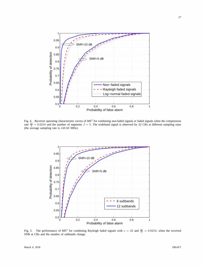
Fig. 4 shows the receiver operating characteristic (ROC) curves of MS3 when combining non-

faded and faded signals. When the average SNR as received at CRs is 5 dB, the performance of

MS3 combining faded signals is roughly the same as that of combining non-faded signals. This

is because the strength of the signal is mostly masked by the noise. In contrast, the detection

performance of MS3 combining non-faded signals outperforms that of combiningfaded signals

when SNR=10 dB. In addition, it is seen that the performance of MS3 combining log-normal

shadowed signals is the poorest. Nonetheless, even for log-normal shadowed signals, MS3 has a

probability of nearly90% for detecting the presence of PUs when the probability of false alarm

is 10%, with the compression rate ofMN

= 0.0219. To investigate the influence ofs and SNR,

we use Fig. 5 to show the performance of MS3 when the received signals are faded according

to Rayleigh distribution with different values ofs (proportional to the number of subbands). We

see that, as the number of subbands decreases, the detectionperformance improves for the same

SNR. The performance improvement of MS3 stems from that, for a fixed number of sampling

channels, decreasings makes it easier to distinguish the occupied frequencies from the aliased

frequencies as discussions in Section III-C.

Fig. 6(a) depicts the influence of the standard deviation when the MS3 system combines

log-normal shadowed signals. It can be seen that a larger standard deviation will lead to worse

detection performance for the MS3 system. It is because a largerσ is equivalent to a longer tail in

March 4, 2018 DRAFT

18

the log-normal distribution, thus making the detection more difficult. In Fig. 6(b), we compare

the performance of MS3 with that of Nyquist systems. In the Nyquist system type I, each

CR is given an orthogonal subband (wideband spectrum is divided into several equal-length

subbands) to sense using Nyquist rate, while their decisions are sent back to the FC. In the

Nyquist system type II, we assume that each CR must sense all wideband spectrum non-

cooperatively, thus requiring multiple standard ADCs in each node to cover all wideband

spectrum. After signal sampling, all measurements are sentback to the FC, where equal

gain combining approach is adopted to fuse data and then energy detection is used for

spectrum sensing. Fig. 6(b) shows that the proposed system has superior performance to

the Nyquist system type I, but inferior performance to the Nyquist system type II. The poor

performance of the Nyquist system type I mainly results fromthe lack of spatial diversity

gain. In the Nyquist system type I, each subband is only sensed by one CR as each CR is

given an orthogonal subband to sense, which cannot take advantage of spatial diversity.

In contrast, both the proposed system and the Nyquist systemtype II are monitoring each

subband using several CRs, thus taking advantage of spatialdiversity. It can also be seen

that the Nyquist system type II has marginal performance gain over the proposed system,

however, at the expense of much higher implementation complexity as discussed below.

In Table I, we compare the implementation complexity of MS3 with that of the Nyquist

systems, when the received signals at different CRs are faded according to Rayleigh distribution.

Here, we consider the comparison metric: the number of same-sampling-rate ADCs for achieving

Pd ≥ 90% andPf ≤ 10%, because practical CRs often have requirements on the probabilities

of detection and false alarm to secure the performance of both CRs and PUs. We can see that,

when there exist 10 CRs, MS3 requires each CR equipped with a single ADC with an average

sampling rate of957.54 MHz; thus, the whole CR network only requires 10 low-rate ADCs. In

contrast, the Nyquist system type I requires 21 ADCs in total, because of21×957.54 MHz≈ 20

GHz for covering10 GHz spectrum based on Nyquist sampling theorem. In the Nyquist system

type II, 210 ADCs (with the average sampling rate957.54 MHz) will be required because each

CR will require 21 ADCs similar to the Nyquist system type I.Thus, the system complexity

March 4, 2018 DRAFT

19

of MS3 is approximately half of that of the Nyquist system type I andmuch less than that

of the Nyquist system type II.

In Fig. 7, we choose the CS-based system in [13] as a benchmarksystem due to its high

impact and outstanding performance. The comparison between the proposed MS3 system and

the benchmark system is provided. We assume thatv = 22 CRs are collaborating for wideband

spectrum sensing in both systems, in order to increase the reliability of spectrum sensing by

exploiting spatial diversity. We can see from Fig. 7(a) thatMS3 outperforms the CS-based system

for every compression rate.In Fig. 7(b), it is seen that, compared with the benchmark system,

MS3 has better compression capability. Using MS3, the probability of successful sensing

becomes larger than90% when the compression rateMN

≥ 0.023. In contrast, the benchmark

system can achieve the probability of successful sensing90% only when the compression

rate MN

≥ 0.045. Furthermore, as shown in Table II, we can find that the computational

complexity of MS3 is O(N logN) due to the energy detection with FFT operations, rather than

O (N(M + logN)) in the CS-based system, whereM is usually much larger thanlogN . The

complexity of the CS-based system is caused by both the matrix multiplication operations and the

FFT operations for spectral recovery. To sum up, with the same computational resources, MS3

has a relatively smaller spectrum sensing overhead than theCS-based system, not only because

of the better compression capability (less data transmission results in shorter transmission time),

but also due to the lower computational complexity.

VI. CONCLUSIONS

In this paper, we have presented a novel system, i.e., MS3, for wideband spectrum sensing

in CR networks. MS3 can relax the wideband spectrum sensing requirements of CRsdue to

its capability of sub-Nyquist sampling. It has been shown that, using sub-Nyquist samples, the

wideband spectrum can be sensed in a collaborative manner without spectral recovery, leading

to a high energy-efficiency and a low spectrum sensing overhead. Moreover, we have derived

closed-form bounds for the performance of MS3 when combining faded or shadowed signals.

Simulation results have verified the derived bounds on the probabilities of false alarm and

March 4, 2018 DRAFT

20

detection. It has also been shown that using partial measurements, MS3 has superior performance

even under low SNR scenarios. The performance of MS3 improves as either the number of CRs

or the average sampling rate increases. Compared to the existing wideband spectrum sensing

methods, MS3 not only provides computation and memory savings, but also reduces the hardware

acquisition requirements and the energy costs at CRs.

APPENDIX A

RELATIONSHIP BETWEENNYQUIST DFT SPECTRUM AND SUB-NYQUIST DFT SPECTRUM

Using the Poisson summation formula [29], (9), and (10), we obtain:

fi∑

l∈ZXc,i(w + fil) =

∑

n∈Zyi[n]e

−2πwn =

Mi−1∑

n=0

yi[n]e−2πwn = Yi(w) (45)

whereXc,i(w) =∫∞−∞ xc,i(t)e

−2πwtdt. Similar to (45), by using (1) and (2), we can obtain:

f∑

l∈ZXc,i(w + fl) =

∑

n∈Zxi[n]e

−2πwn =

N−1∑

n=0

xi[n]e−2πwn = Xi(w). (46)

As the received signal is bandlimited andf ≥ 2W , Xi(w) = fXc,i(w) holds forw ∈ [−W2, W

2].

Substituting it to (45), we obtainYi(w) =fif

∑∞l=−∞Xi(w+ fil). In a discrete form, we end up

with:

Yi[m] =Mi

N

∞∑

l=−∞Xi[m+ lMi], m = 0, 1, · · · ,Mi − 1. (47)

APPENDIX B

PROBABILITY OF SIGNAL OVERLAP AT SUB-NYQUIST SAMPLING

As s spectral components are distributed over the frequency bins of 0, 1, · · · , N − 1, the

probability of the frequency bink belonging to the spectral supportΩ is P = Pr(k ∈ Ω) = sN

.

Let q denote the number of spectral components overlapped on the frequency binm, using (11)

the probability of no signal overlap is given by

Pr(q < 2) = Pr(q = 0)+Pr(q = 1) = (1−P )⌈NMi

⌉+

(⌈ NMi

⌉1

)P (1−P )⌈

NMi

⌉−1 (48)

March 4, 2018 DRAFT

21

where ⌈ NMi

⌉ denotes the number of summations in (11). SubstitutingP = sN

into (48) while

choosing sub-Nyquist sampling rate in MS3 such thatMi =√N , we obtain

Pr(q < 2) =

(N−sN

) NMi

+s

Mi

(N−sN

)N−MiMi

=(N−sN

)√N (N−s+s

√N)

N−s . (49)

It can be tested thatPr(q < 2) approaches to 1 when choosingN such thatN ≫ s. Thus the

probability of signal overlap approaches to zero under the condition we choose.

APPENDIX C

PROOF OFLEMMA 1

Let Mi andMj denote the number of samples at CRsi and j, respectively. Using (12) and

(20), we can represent the aliased frequencies projected from k1 ∈ Ω by

gi = |k1| mod (Mi) + lMi = k1 − hMi + lMi, h 6= l (50)

gj = |k1| mod (Mj) + lMj = k1 − hMj + lMj , h 6= l (51)

where integersh andh are quotients from modulo operations, andl−h ∈ [−⌈ NMi

⌉+1, ⌈ NMi

⌉−1],

l − h ∈ [−⌈ NMj

⌉+ 1, ⌈ NMj

⌉ − 1], in which ⌈ NMi

⌉ gives the smallest integer not less thanNMi

.

Avoiding gi = gj is equivalent to avoiding(l − h)Mi = (l − h)Mj . If Mi and Mj are

different primes, the conditionmax(|l− h|) < Mj (i.e., ⌈ NMi

⌉ − 1 < Mj) will satisfy this. After

simplification, the conditionMiMj > N is obtained. Moreover, if it holds for any two CRs, the

case for more than two CRs will also hold.

APPENDIX D

PROOF OFTHEOREM 2

If the received signals at CRs are Rayleigh faded, the lower bound on the average probability

of false alarm will remain as it is independent of the SNR. Using (25), (27), and (28), the upper

bound on the average probability of false alarm can be calculated by

Pf,kup=

∫ ∞

0

QJv

(√ψγs,

√λk

) γs−1s

γsΓ(s)e−

γsγ dγs. (52)

March 4, 2018 DRAFT

22

Rewriting the Marcum Q-function by using (4.74) in [35] and (8.352-2) in [36], we obtain:

QJv

(√ψγs,

√λk

)=

∞∑

n=0

(ψγs

2

)ne−

ψγs2

n!

Γ(n+ Jv, λk2)

Γ(n+ Jv). (53)

Substituting (53) into (52), we can rewrite (52) as

Pf,kup=

1

γs

∞∑

n=0

(ψ2

)nΓ(n+ Jv, λk

2)

n!(s− 1)!Γ(n+ Jv)

∫ ∞

0

γn+s−1s e−

ψγs2

− γsγ dγs. (54)

Calculating the integral by using (3.351-3) in [36], we end up with

Pf,kup=

(1 +

ψγ

2

)−s ∞∑

n=0

Cnn+s−1

(ψγ

ψγ + 2

)n Γ(n+ Jv, λk

2

)

Γ (n + Jv). (55)

Similarly, we can obtain the lower bound on the average probability of detection.

APPENDIX E

PROOF OFTHEOREM 3

If the received signals are shadowed according to log-normal distribution, the lower bound

on Pf,k in (40) will remain. By (38), the upper bound on the probability of false alarm can be

given by

Pf,ku=

∫ ∞

0

QJv

(√ψγs,

√λk

)√ sη

2πγ−3/2

s exp

(−η(γs − sθ)2

2sθ2γs

)dγs. (56)

Substituting (53) into (56), we calculatePf,ku

as

Pf,ku=

√sη

2π

∞∑

n=0

(ψ2

)nΓ(n + Jv, λk

2

)

n!Γ (n+ Jv)

∫ ∞

0

γn− 3

2s exp

(−sψθ

2 + η

2sθ2γs −

sη

2γs+η

θ

)dγs. (57)

Using (3.471-9) in [36] for calculating the integral in (57), we obtain

Pf,ku=

√2sη

πeηθ

∞∑

n=0

(ψ2

)nΓ(n + Jv, λk

2

)

n!Γ (n+ Jv)

(√s2ηθ2

sψθ2 + η

)n− 1

2

Kn− 1

2

(√η(sψθ2 + η)

θ2

). (58)

Likewise, the lower bound on the average probability of detection can be approximated.

REFERENCES

[1] M. A. McHenry, “NSF spectrum occupancy measurements project summary,” Shared Spectrum Company, Tech. Rep.,

Aug. 2005.

[2] S. Stotas and A. Nallanathan, “On the outage capacity of sensing-enhanced spectrum sharing cognitive radio systemsin

fading channels,”IEEE Transactions on Communications, vol. 59, no. 10, pp. 2871–2882, October 2011.

March 4, 2018 DRAFT

23

[3] Z. Chen, C.-X. Wang, X. Hong, J. Thompson, S. Vorobyov, X.Ge, H. Xiao, and F. Zhao, “Aggregate interference modeling

in cognitive radio networks with power and contention control,” IEEE Transactions on Communications, vol. 60, no. 2,

pp. 456–468, Feb. 2012.

[4] H. Sun, D. I. Laurenson, J. S. Thompson, and C.-X. Wang, “Anovel centralized network for sensing spectrum in cognitive

radio,” in Proc. IEEE International Conference on Communications, Beijing, China, May 2008, pp. 4186–4190.

[5] Q. Chen, M. Motani, W.-C. Wong, and A. Nallanathan, “Cooperative spectrum sensing strategies for cognitive radio mesh

networks,” IEEE Journal on Selected Topics in Signal Processing, vol. 5, no. 1, pp. 56–67, Feb. 2011.

[6] M.-H. Yoon, Y. Shin, H.-K. Ryu, and J.-M. Woo, “Ultra-wideband loop antenna,”Electronics Letters, vol. 46, no. 18, pp.

1249–1251, Sept. 2010.

[7] Z.-C. Hao and J.-S. Hong, “Highly selective ultra wideband bandpass filters with quasi-elliptic function response,” IET

Microwaves, Antennas Propagation, vol. 5, no. 9, pp. 1103–1108, 2011.

[8] A. Bevilacqua and A. M. Niknejad, “An ultrawideband CMOSlow-noise amplifier for 3.1-10.6-GHz wireless receivers,”

IEEE Journal of Solid-State Circuits, vol. 39, no. 12, pp. 2259–2268, Dec. 2004.

[9] [Online]. Available: www.national.com/pf/DC/ADC12D1800.html

[10] Z. Quan, S. Cui, A. H. Sayed, and H. V. Poor, “Optimal multiband joint detection for spectrum sensing in cognitive radio

networks,” IEEE Transactions on Signal Processing, vol. 57, no. 3, pp. 1128–1140, Mar. 2009.

[11] ——, “Wideband spectrum sensing in cognitive radio networks,” in Proc. IEEE International Conference on Communica-

tions, Beijing, China, May 2008, pp. 901–906.

[12] Z. Tian and G. B. Giannakis, “A wavelet approach to wideband spectrum sensing for cognitive radios,” inProc. IEEE

Cognitive Radio Oriented Wireless Networks and Communications, Mykonos Island, Greece, June 2006, pp. 1–5.

[13] ——, “Compressed sensing for wideband cognitive radios,” in Proc. IEEE International Conference on Acoustics, Speech,

and Signal Processing, Hawaii, USA, April 2007, pp. 1357–1360.

[14] Z. Tian, Y. Tafesse, and B. M. Sadler, “Cyclic feature detection with sub-nyquist sampling for wideband spectrum sensing,”

IEEE Journal of Selected Topics in Signal Processing, vol. 6, no. 1, pp. 58–69, Feb. 2012.

[15] F. Zeng, C. Li, and Z. Tian, “Distributed compressive spectrum sensing in cooperative multihop cognitive networks,” IEEE

Journal of Selected Topics in Signal Processing, vol. 5, no. 1, pp. 37–48, Feb. 2011.

[16] Y. Wang, Z. Tian, and C. Feng, “Sparsity order estimation and its application in compressive spectrum sensing for cognitive

radios,” IEEE Transactions on Wireless Communications, vol. 11, no. 6, pp. 2116–2125, June 2012.

[17] Y. L. Polo, Y. Wang, A. Pandharipande, and G. Leus, “Compressive wide-band spectrum sensing,” inProc. IEEE

International Conference on Acoustics, Speech, and SignalProcessing, Taipei, April 2009, pp. 2337–2340.

[18] H. Sun, A. Nallanathan, J. Jiang, D. I. Laurenson, C.-X.Wang, and H. V. Poor, “A novel wideband spectrum sensing

system for distributed cognitive radio networks,” inProc. IEEE Global Telecommunications Conference, Houston, TX,

USA, Dec. 2011, pp. 1–6.

[19] Y. Wang, A. Pandharipande, and G. Leus, “Compressive sampling based MVDR spectrum sensing,” in2010 2nd

International Workshop on Cognitive Information Processing (CIP), June 2010, pp. 333–337.

[20] V. Havary-Nassab, S. Hassan, and S. Valaee, “Compressive detection for wide-band spectrum sensing,” inin Proc. of IEEE

Int. Conf. Acoustics, Speech and Signal Processing (ICASSP2010), Dallas, TX, USA, Mar. 2010, pp. 3094–3097.

March 4, 2018 DRAFT

24

[21] U. Nakarmi and N. Rahnavard, “Joint wideband spectrum sensing in frequency overlapping cognitive radio networks using

distributed compressive sensing,” inProc. Military Communications Conference, Baltimore, MD, USA, Nov. 2011, pp.

1035–1040.

[22] Y. Zhang, Y. Liu, and Q. Wan, “Fast compressive widebandspectrum sensing based on dictionary linear combination,”in

Proc. IEEE WiCOM, Wuhan, China, Sept. 2011, pp. 1–4.

[23] D. D. Ariananda and G. Leus, “Compressive wideband power spectrum estimation,”IEEE Transactions on Signal

Processing, vol. 60, no. 9, pp. 4775–4789, sept. 2012.

[24] Y. Liu and Q. Wan, “Enhanced compressive wideband frequency spectrum sensing for dynamic spectrum access,”EURASIP

Journal on Advances in Signal Processing, vol. 2012(177), 2012.

[25] H. Sun, A. Nallanathan, and J. Jiang, “Adaptive compressive spectrum sensing in distributed cognitive radio networks,” in

Proc. IEEE Asia Pacific Wireless Communication Symposium, Singapore, August 2011, pp. 1–5.

[26] H. Sun, A. Nallanathan, J. Jiang, and H. V. Poor, “Compressive autonomous sensing (CASe) for wideband spectrum

sensing,” inProc. of IEEE International Conference on Communications, Ottawa, Canada, June 2012, pp. 5953–5957.

[27] H. Sun, D. Laurenson, and C.-X. Wang, “Computationallytractable model of energy detection performance over slow

fading channels,”IEEE Communications Letters, vol. 14, no. 10, pp. 924–926, Oct. 2010.

[28] H. Su and X. Zhang, “Cross-layer based opportunistic MAC protocols for QoS provisionings over cognitive radio wireless

networks,” IEEE Journal on Selected Areas in Communications, vol. 26, no. 1, pp. 118–129, 2008.

[29] M. A. Pinsky, Introduction to Fourier Analysis and Wavelets. Providence, Rhode Island, USA: American Mathematical

Society, 2002.

[30] P. Cantrell and A. Ojha, “Comparison of generalized Q-function algorithms,”IEEE Transactions on Information Theory,

vol. 33, no. 4, pp. 591–596, July 1987.

[31] C. W. Helstrom, “Approximate inversion of Marcum’s Q-function,” IEEE Transactions on Aerospace and Electronic

Systems, vol. 34, no. 1, pp. 317–319, Jan. 1998.

[32] A. H. Marcus, “Power sum distributions: an easier approach using the Wald distribution,”Journal of American Statistical

Association, vol. 71, pp. 237–238, 1976.

[33] R. S. Chhikara and J. L. Folks,The Inverse Gaussian Distribution: Theory, Methodology, and Applications. New York:

Marcel Dekker Inc., 1989.

[34] M. Mishali and Y. Eldar, “From theory to practice: Sub-Nyquist sampling of sparse wideband analog signals,”IEEE

Journal of Selected Topics in Signal Processing, vol. 4, no. 2, pp. 375 –391, april 2010.

[35] M. K. Simon and M.-S. Alouini,Digital Communication over Fading Channels, 2nd ed. New York: John Wiley & Sons,

Inc., Dec. 2004.

[36] I. S. Gradshteyn and I. M. Ryzhik,Table of Integrals, Series, and Products, 5th ed., A. Jeffrey, Ed. New York: Academic

Press, Inc., 1994.

March 4, 2018 DRAFT

25

Sub-Nyquist

Sampling

Signal

Energy

Sub-Nyquist

Sampling

Signal

Energy

Sub-Nyquist

Sampling

Signal

Energy

Cognitive Radio 1

Cognitive Radio 2

Cognitive Radio v

Wideband

Filter

Wideband

Filter

Wideband

Filter

H0,k

H1,k

,s vE

!

,2sE

!

,1sE

!

FFT

FFT

FFT

1Y

!

2Y

!

vY

!

Hypothesis

Test

Fusion Center

Data

Fusion

sE

Fig. 1. Block diagram of multi-rate sub-Nyquist spectrum sensing (MS3) system.

0 0.5 1 1.5 2 2.5 3 3.5 4

x 104

0

5

10x 10

6

Frequency

Mag

nitu

de

(a) Spectrum in Nyquist Sampling System

0 0.5 1 1.5 2 2.5 3 3.5 4

x 104

0

5

10x 10

11

Frequency

Mag

nitu

de

(b) Test Statistic in Proposed MS3 System

Fig. 2. Illustration of the proposed system for sensing practical ASTC DTV signal: (a) Spectrum of an ASTC DTVsignal in Nyquist sampling system, and (b) Test statistic inthe proposed system. Here, we use ASTC DTV signalWAS 3 27 06022000 REF and assume the number of CRsv = 22. The number of Nyquist samples isN = 80, 000, andthe numbers of sub-Nyquist samples in MS3 system are consecutive primesM1 = 1613, M2 = 1619, · · · ,M22 = 1783. Theaverage compression rate is calculated toM

N= 2.12%.

March 4, 2018 DRAFT

26

1.2 1.4 1.6 1.8 2 2.2 2.4

x 107

0

0.2

0.4

0.6

0.8

1

Threshold (λ)(b)

Pro

ba

bili

ty

Simulated Pf

Simulated Pd

Lower bound of Pf

Upper bound of Pf

Lower bound of Pd

1.2 1.4 1.6 1.8 2 2.2 2.4

x 107

0

0.2

0.4

0.6

0.8

1

Threshold (λ)(a)

Pro

ba

bili

ty

Simulated Pf

Simulated Pd

Lower bound of Pf

Upper bound of Pf

Lower bound of Pd

1.2 1.4 1.6 1.8 2 2.2 2.4 2.6

x 107

0

0.2

0.4

0.6

0.8

1

Threshold (λ)(c)

Pro

ba

bili

ty

Simulated Pf

Simulated Pd

Lower bound of Pf

Upper bound of Pf

Lower bound of Pd

Fig. 3. Comparisons of simulation results and analytical results for the probabilities of false alarm and detection when MS3

combining (a)non-faded signals, (b) Rayleigh faded signals, and (c) Log-normal shadowed signals with the received SNR= 5dB (at CRs) andσ = 4 dB.

March 4, 2018 DRAFT

27

0 0.2 0.4 0.6 0.8 10.5

0.55

0.6

0.65

0.7

0.75

0.8

0.85

0.9

0.95

1

Probability of false alarm

Pro

babi

lity

of d

etec

tion

Non−faded signalsRayleigh faded signalsLog−normal faded signals

SNR=5 dB

SNR=10 dB

Fig. 4. Receiver operating characteristic curves of MS3 for combining non-faded signals or faded signals when the compressionrate M

N= 0.0219 and the number of segmentsJ = 5. The wideband signal is observed by22 CRs at different sampling rates

(the average sampling rate is448.68 MHz).

0 0.2 0.4 0.6 0.8 10.5

0.55

0.6

0.65

0.7

0.75

0.8

0.85

0.9

0.95

1

Probability of false alarm

Pro

babi

lity

of d

etec

tion

6 subbands

12 subbands

SNR=10 dB

SNR=5 dB

Fig. 5. The performance of MS3 for combining Rayleigh faded signals withv = 22 and MN

= 0.0219, when the receivedSNR at CRs and the number of subbands change.

March 4, 2018 DRAFT

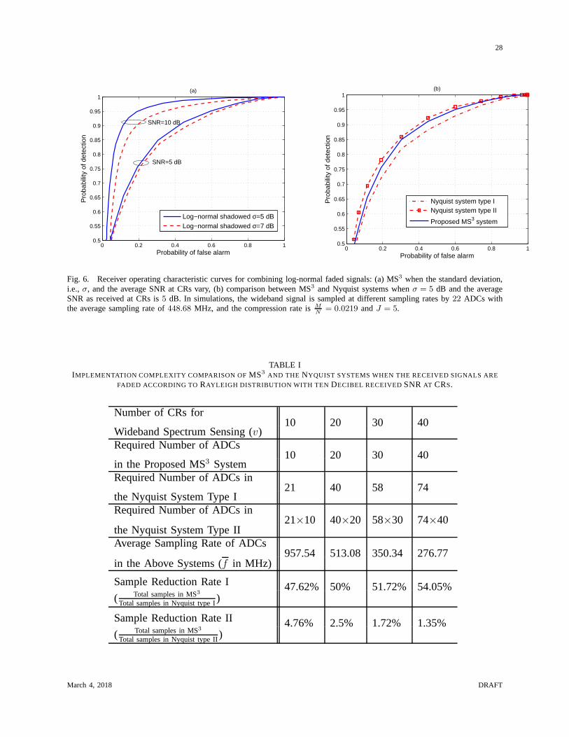
28

0 0.2 0.4 0.6 0.8 10.5

0.55

0.6

0.65

0.7

0.75

0.8

0.85

0.9

0.95

1

Probability of false alarm

Pro

babi

lity

of d

etec

tion

(a)

Log−normal shadowed σ=5 dBLog−normal shadowed σ=7 dB

SNR=10 dB

SNR=5 dB

0 0.2 0.4 0.6 0.8 10.5

0.55

0.6

0.65

0.7

0.75

0.8

0.85

0.9

0.95

1

Probability of false alarm

Pro

babi

lity

of d

etec

tion

(b)

Nyquist system type INyquist system type II

Proposed MS3 system

Fig. 6. Receiver operating characteristic curves for combining log-normal faded signals: (a) MS3 when the standard deviation,i.e., σ, and the average SNR at CRs vary, (b) comparison between MS3 and Nyquist systems whenσ = 5 dB and the averageSNR as received at CRs is5 dB. In simulations, the wideband signal is sampled at different sampling rates by22 ADCs withthe average sampling rate of448.68 MHz, and the compression rate isM

N= 0.0219 andJ = 5.

TABLE IIMPLEMENTATION COMPLEXITY COMPARISON OFMS3 AND THE NYQUIST SYSTEMS WHEN THE RECEIVED SIGNALS ARE

FADED ACCORDING TORAYLEIGH DISTRIBUTION WITH TEN DECIBEL RECEIVEDSNRAT CRS.

Number of CRs for10 20 30 40

Wideband Spectrum Sensing (v)Required Number of ADCs

10 20 30 40in the Proposed MS3 SystemRequired Number of ADCs in

21 40 58 74the Nyquist System Type IRequired Number of ADCs in

21×10 40×20 58×30 74×40the Nyquist System Type IIAverage Sampling Rate of ADCs

957.54 513.08 350.34 276.77in the Above Systems (f in MHz)

Sample Reduction Rate I 47.62% 50% 51.72% 54.05%( Total samples in MS3

Total samples in Nyquist type I)

Sample Reduction Rate II 4.76% 2.5% 1.72% 1.35%( Total samples in MS3

Total samples in Nyquist type II)

March 4, 2018 DRAFT

29

0 0.01 0.02 0.03 0.04 0.050.5

0.55

0.6

0.65

0.7

0.75

0.8

0.85

0.9

0.95

1

Compression rate (M/N)

Pro

babi

lity

of d

etec

tion

(a)

Proposed MS3 system

Traditional CS system [13]

0 0.01 0.02 0.03 0.04 0.050

0.1

0.2

0.3

0.4

0.5

0.6

0.7

0.8

0.9

1

Compression rate (M/N)

Pro

babi

lity

of s

uces

sful

sen

sing

(b)

ProposedMS3 system

TraditionalCS system [13]

Fig. 7. Comparison between MS3 and CS-based system [13]: (a) the probability of detection when the probability of falsealarm is set to10%, and (b) the probability of successful sensing which is defined as the probability of achieving bothPd ≥ 90%andPf ≤ 10%. In simulations, the average SNR as received at CRs is10 dB and the number of CRs isv = 22.

TABLE IICOMPARISONS OF WIDEBAND SPECTRUM SENSING TECHNIQUES.

ApproachCompression ADC/DSP Implementation Computational

Capability Type Complexity Complexity

Wavelet detection × Nyquist low O(N logN)

Multiband joint detection × Nyquist high O (N logN)

CS-based detection√

sub-Nyquist medium O (N(M + logN))

Proposed system√

sub-Nyquist low O(N logN)

March 4, 2018 DRAFT