1

MEASUREMENT THEORY AND ITS APPLICATIONS

FRED S. ROBERTS RUTGERS UNIVERSITY

2

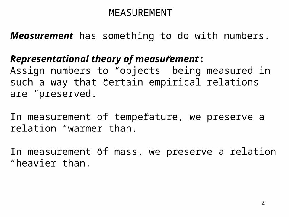
MEASUREMENT

Measurement has something to do with numbers.

Representational theory of measurement:Assign numbers to “objects” being measured in such a way that certain empirical relations are “preserved.”

In measurement of temperature, we preserve a relation “warmer than.”

In measurement of mass, we preserve a relation “heavier than.”

3

A: set of objects R : binary relation on A

R could be preference. Then f is a utility function (ordinal utility function).

In mass, there is more going on: There is an operation of combination of objects and mass is additive: means a combined with b:

a±b

f (a±b) = f (a) + f (b):

aRb$ a is warmer than b

aRb$ a is heavier than b:

f : A ! R

aRb$ f (a) > f (b):

4

Homomorphisms Relational System:

A set Ri relation on A (not necessarily binary) operation on A (binary)

Homomorphism from into

is a function such that

±i

f : A ! B

(a1;a2; :::;ami) 2 R i $

(f (a1); f (a2); :::; f (ami)) 2 R0

i

f (a±j b) = f (a) ±0j f (b):

A = (A;R1;R2;:::;Rp;±1;±2; :::;±q)

B = (B;R01;R

02; :::;R

0p;±

01;±

02; :::;±

0q)

A

5

(This only makes sense if Ri and are both )

Examples of Homomorphisms

Example 1: Let a mod 3 be the number b in {0,1,2} such that (mod 3). Let A = {0,1,2,…,26} and

Then f(a) = a mod 3 is a homomorphism from (A,R) into

f(11) = 2, f(6) = 0, ...

a´ b

(R;>):

R0i mi ¡ ary:)

aRb$ a mod 3> bmod 3.

6

Example 2: A = {a,b,c,d}R = {(a,b),(b,c),(a,c),(a,d),(b,d),(c,d)}f(a) = 4, f(b) = 3, f(c) = 2, f(d) = 1.

f is a homomorphism from (A, R) into

Second homomorphism: g(a) = 10, g(b) = 4, g(c) = 2, g(d) = 0.

Example 3: A = {a,b,c}, R = {(a,b),(b,c),(c,a)}

There is no homomorphism

Therefore, f(a) > f(c): But cRa f(c) > f(a).

(R;>):

f : (A;R) ! (R;>):

aRb! f (a) > f (b); bRc! f (b) > f (c)

7

Example 4: A = {0,1,2,…}, B = {0,2,4,…}

A homomorphism f(a) = 2a

f(a + b) = f(a) + f(b).

Second homomorphism: g(a) = 4a: A homomorphism does not have to be onto.

Example 5: A homomorphism

f(a) = ea

f : (A;>;+) ! (B;>;+) :

f : (R;>;+) ! (R+;>;£) :

a>bÃ! f (a)>f (b)f (a+b) = ea+b=eaeb= f (a) £ f (b):

a> b$ f (a) > f (b)

8

Temperature Measurement: homomorphism

Mass Measurement: homomorphism

Since negative numbers do not arise in the case of mass, we can think of the homomorphism as being into

The Two Problems of Representational Measurement Theory

Representation Problem: Find conditions on (necessary) and sufficient for the existence of a homomorphism from into .

Subproblem: Find an algorithm for obtaining the homomorphism.

(A;R) ! (R;>)

(A;R;±) ! (R;>;+):

(R+;>;+):

A

A

9

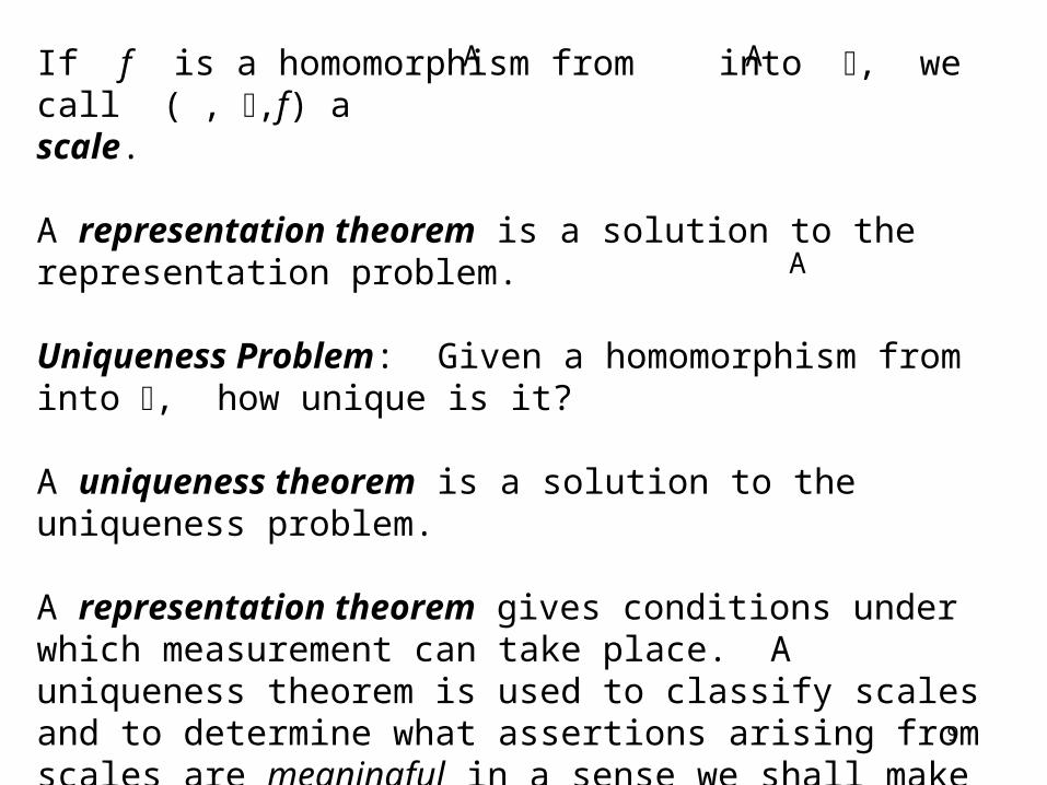
If f is a homomorphism from into , we call ( , ,f) a scale.

A representation theorem is a solution to the representation problem.

Uniqueness Problem: Given a homomorphism from into , how unique is it?

A uniqueness theorem is a solution to the uniqueness problem.

A representation theorem gives conditions under which measurement can take place. A uniqueness theorem is used to classify scales and to determine what assertions arising from scales are meaningful in a sense we shall make precise.

A A

A

10

The Theory of Uniqueness

Admissible Transformations

An admissible transformation sends one acceptable scale into another.

In most cases one can think of an admissible transformation as defined on the range of a homomorphism.

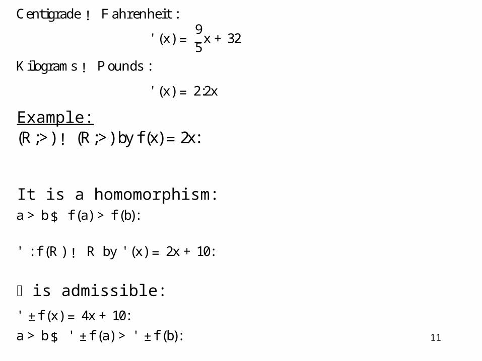
Suppose f is a homomorphism from into .

is called an admissible transformation of f if is again a homomorphism from into .' : f (A) ! B ' ±f

Centigrade ! F ahrenheit

Kilograms ! Pounds

A

A

11

Example:

It is a homomorphism:

is admissible:

(R;>) ! (R;>) byf (x)=2x:

' (x) =95x+32

' (x) = 2:2x

' : f (R ) ! R by ' (x) = 2x+10:

' ±f (x) = 4x+10:

Centigrade ! F ahrenheit :

K ilograms ! Pounds :

a> b$ f (a) > f (b):

a> b$ ' ±f (a) > ' ±f (b):

12

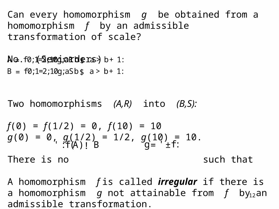
Can every homomorphism g be obtained from a homomorphism f by an admissible transformation of scale?

No. (Semiorders)

Two homomorphisms (A,R) into (B,S):

f(0) = f(1/2) = 0, f(10) = 10g(0) = 0, g(1/2) = 1/2, g(10) = 10.

There is no such that

A homomorphism f is called irregular if there is a homomorphism g not attainable from f by an admissible transformation.

' : f (A) ! B g=' ±f:

A = f0;1=2;10g;aRb$ a> b+1:

B = f0;1=2;10g;aSb$ a> b+1:

13

Irregular scales are unusual and annoying. We shall assume (until later) that all scales are regular. Most common scales of measurement are. In the case where all scales are regular, we can develop the theory of uniqueness by studying admissible transformations.

A classification of scales is obtained by studying the class of admissible transformations associated with the scale. This defines the scale type. (S.S. Stevens)

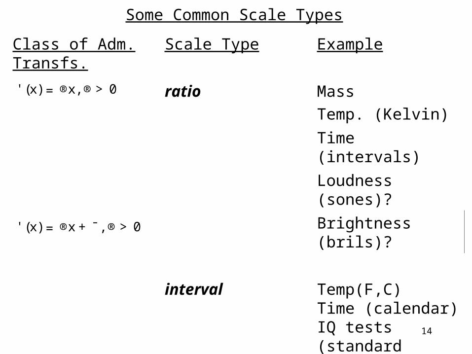
14

Some Common Scale Types

Class of Adm. Transfs.

Scale Type Example

ratio Mass

Temp. (Kelvin)

Time (intervals)

Loudness (sones)?

Brightness (brils)?

interval Temp(F,C)Time (calendar)IQ tests (standard scores?)

' (x) =®x, ®>0

' (x) =®x+¯, ®> 0

15

Class of Adm. Transfs.

Scale Type Example

strictly increasing

ordinal Preference?

Hardness

Grades of leather, wool, etc.

IQ tests (raw scores)?

absolute Counting' (x) = x

x ¸ y $ ' (x) ¸ ' (y)

16

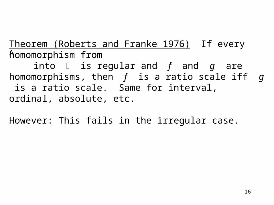
Theorem (Roberts and Franke 1976) If every homomorphism from into is regular and f and g are homomorphisms, then f is a ratio scale iff g is a ratio scale. Same for interval, ordinal, absolute, etc.

However: This fails in the irregular case.

A

17

Meaningful Statements

In measurement theory, we speak of a statement as being meaningful if its truth or falsity is not an artifact of the particular scale values used.

Assuming all scales involved are regular, one can use the following definition (due to Suppes 1959 and Suppes and Zinnes 1963).

Definition: A statement involving numerical scales is meaningful if its truth or falsity is unchanged after any (or all) of the scales is transformed (independently?) by an admissible transformation.

18

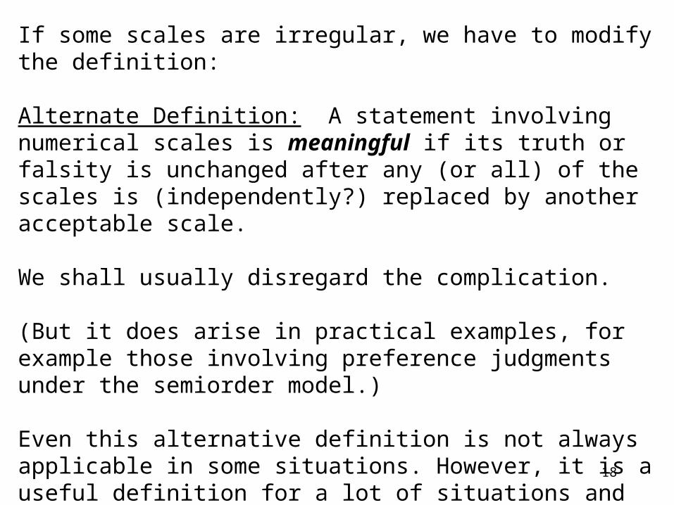
If some scales are irregular, we have to modify the definition:

Alternate Definition: A statement involving numerical scales is meaningful if its truth or falsity is unchanged after any (or all) of thescales is (independently?) replaced by another acceptable scale.

We shall usually disregard the complication.

(But it does arise in practical examples, for example those involving preference judgments under the semiorder model.)

Even this alternative definition is not always applicable in some situations. However, it is a useful definition for a lot of situations and we shall adopt it.

19

“This talk will be three times as long as the previous talk.”

Is this meaningful?We have a ratio scale (time intervals).

(1) f(a) = 3f(b).

This is meaningful if f is a ratio scale. For, an admissible transformation is . We want (1) to hold iff

(2)

But (2) becomes(3)

(1)Ã ! (3) since®>0:

(' ±f )(a) = 3(' ±f )(b):

®f (a) = 3®f (b):

' (x) =®x, ®>0

20

“The high temperature today was three times the high temperature yesterday.”

Meaningless. It could be true with Fahrenheit and false with Centigrade, or vice versa.

In general:For ratio scales, it is meaningful to compare ratios:

f(a)/f(b) > f(c)/f(d)

For interval scales, it is meaningful to compare intervals:

f(a) - f(b) > f(c) - f(d)

For ordinal scales, it is meaningful to compare size:

f(a) > f(b)

21

“I weigh 1000 times what the Statue of Liberty weighs.”

Meaningful. It involves ratio scales.It is false no matter what the unit.

Meaningfulness is different from truth.

It has to do with what kinds of assertions it makes sense to make, which assertions are not accidents of the particular choice of scale (units, zero points) in use.

22

Average Performance

Study two groups of individuals, machines, algorithms, etc. under different conditions.

f(a) is the time required by a to finish a task.

Data suggests that the average performance of individuals in the first group is better than the average performance of individuals in the second group.

individuals in first group individuals in second group.

(1)

We are comparing arithmetic means.

1n

nX

i=1

f (ai ) >1m

mX

i=1

f (bi )

b1, b2, ..., bm

a1, a2, ..., an

23

Statement (1) is meaningful iff for all admissible transformations of scale , (1) holds iff

(2)

Performance = length of time, a ratio scale. Thus, ,so (2) becomes

(3)

Then implies . Hence, (1) is meaningful.

1n

nX

i=1

' ±f (ai ) >1m

mX

i=1

' ±f (bi )

1n

nX

i=1

®f (ai ) >1m

mX

i=1

®f (bi )

®>0

' (x) =®x, ®>0

(1) $ (3)

24

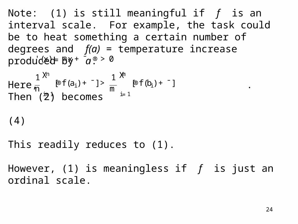
Note: (1) is still meaningful if f is an interval scale. For example, the task could be to heat something a certain number of degrees and f(a) = temperature increase produced by a.

Here, . Then (2) becomes

(4)

This readily reduces to (1).

However, (1) is meaningless if f is just an ordinal scale.

1n

nX

i=1

[®f (ai ) +¯]>1m

mX

i=1

[®f (bi ) +¯]

' (x) =®x+¯, ®> 0

25

To show that comparison of arithmetic means can be meaningless for ordinal scales:

Suppose f(a) is measured on an ordinal scale, e.g., 5-point scale: 5=excellent, 4=very good, 3=good, 2=fair, 1=poor. In such a scale, the numbers don't mean anything, only their order matters.

Group 1: 5, 3, 1 average 3Group 2: 4, 4, 2 average 3.33 (greater)

Admissible transformation: . New scale conveys the same information. New scores:

Group 1: 100, 65, 30 average 65 (greater)Group 2: 75, 75, 40 average 63.33

5! 100, 4! 75, 3! 65, 2! 40, 1! 30

26

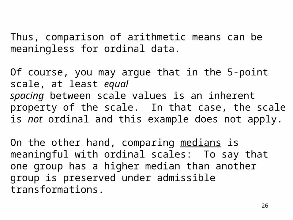
Thus, comparison of arithmetic means can be meaningless for ordinal data.

Of course, you may argue that in the 5-point scale, at least equal spacing between scale values is an inherent property of the scale. In that case, the scale is not ordinal and this example does not apply.

On the other hand, comparing medians is meaningful with ordinal scales: To say that one group has a higher median than another group is preserved under admissible transformations.

27

Importance Ratings/Performance Ratings

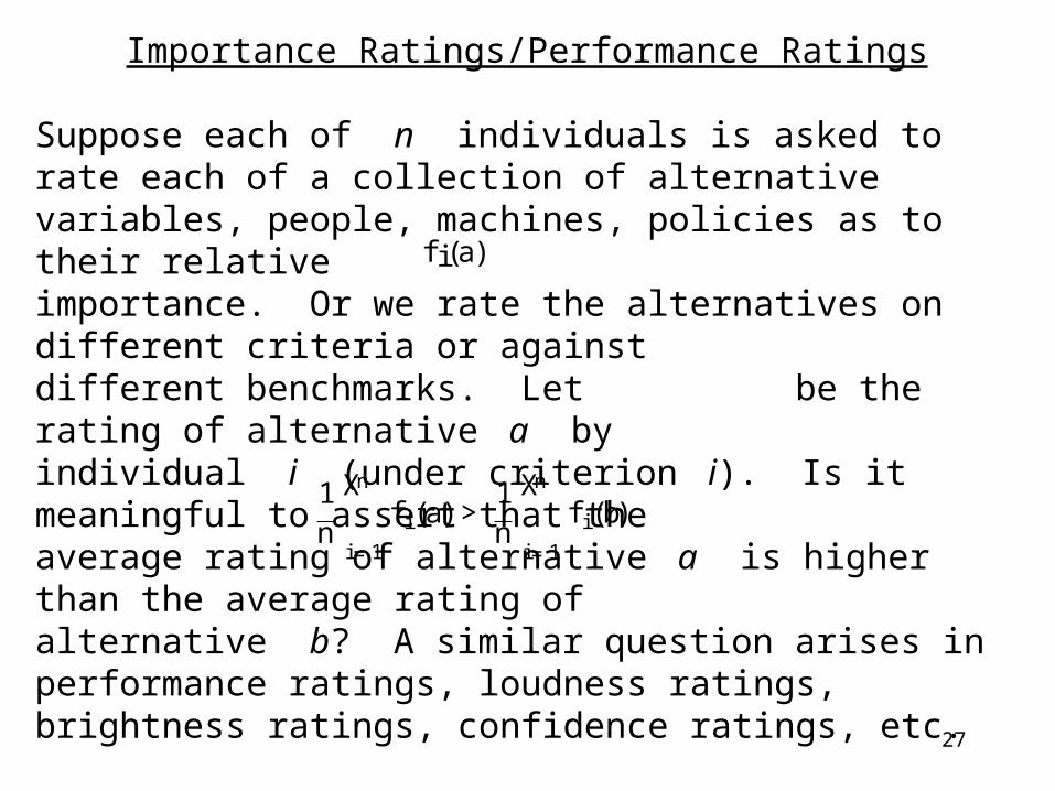
Suppose each of n individuals is asked to rate each of a collection of alternative variables, people, machines, policies as to their relative importance. Or we rate the alternatives on different criteria or against different benchmarks. Let be the rating of alternative a by individual i (under criterion i). Is it meaningful to assert that the average rating of alternative a is higher than the average rating of alternative b? A similar question arises in performance ratings, loudness ratings, brightness ratings, confidence ratings, etc.

(1)

f i(a)

1n

nX

i=1

f i (a) >1n

nX

i=1

f i (b)

28

If each is a ratio scale, then we consider for > 0,

(2)

Clearly, , so (1) is meaningful.

Problem: might have independent units. In this case, we want to allow independent admissible transformations of the . Thus, we must consider

(3)

It is easy to see that there are so that (1) holds and (3) fails. Thus, (1) is meaningless.

f i

1n

nX

i=1

®f i (a) >1n

nX

i=1

®f i (b)

(1)Ã ! (2)

1n

nX

i=1

®i f i (a) >1n

nX

i=1

®i f i (b)

f if 1, f 2, ..., f n

®i

29

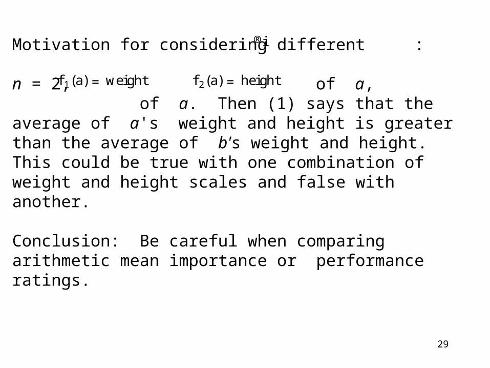
Motivation for considering different :

n = 2, of a, of a. Then (1) says that the average of a's weight and height is greater than the average of b's weight and height. This could be true with one combination of weight and height scales and false with another.

Conclusion: Be careful when comparing arithmetic mean importance or performance ratings.

®i

f 2(a) = heightf 1(a) =weight

30

In this context, it is safer to compare geometric means (Dalkey).

,

all

Thus, if each is a ratio scale, if individuals can change importance rating scales (performance rating scales) independently, then comparison of geometric means is meaningful while comparison of arithmetic means is not.

p¦ ni=1

®i f i (a) >p¦ ni=1

®i f i (b)

®i > 0

f i

p¦ ni=1

f i (a) >p¦ ni=1

f i (b) $n

nn

n

31

Application

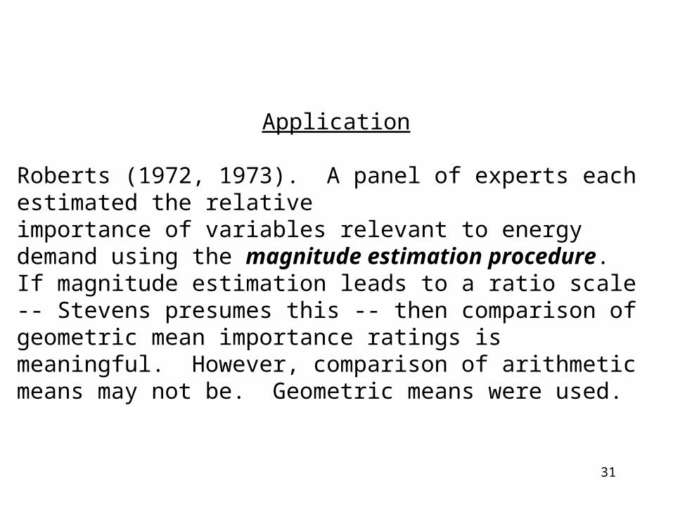
Roberts (1972, 1973). A panel of experts each estimated the relative importance of variables relevant to energy demand using the magnitude estimation procedure. If magnitude estimation leads to a ratio scale -- Stevens presumes this -- then comparison of geometric mean importance ratings is meaningful. However, comparison of arithmetic means may not be. Geometric means were used.

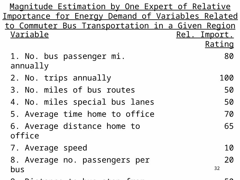
32

Magnitude Estimation by One Expert of Relative Importance for Energy Demand of Variables Related to Commuter Bus Transportation in a

Given RegionVariable Rel. Import. Rating

1. No. bus passenger mi. annually 80

2. No. trips annually 100

3. No. miles of bus routes 50

4. No. miles special bus lanes 50

5. Average time home to office 70

6. Average distance home to office 65

7. Average speed 10

8. Average no. passengers per bus 20

9. Distance to bus stop from home 50

10. No. buses in the region 20

11. No. stops, home to office 20

33

Performance Evaluation

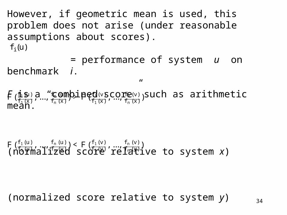
Fleming and Wallace (1986) make a similar point about performance evaluation of computer systems. A number of systems are tested on different benchmarks. Their scores on each benchmark are normalized relative to the score of one of the systems. The normalized scores of a system are combined by some averaging procedure. If the averaging is the arithmetic mean, then the statement that one system has a higher arithmetic mean normalized score than another system is meaningless: The system to which scores are normalized can determine which has the higher arithmetic mean.

34

However, if geometric mean is used, this problem does not arise (under reasonable assumptions about scores).

= performance of system u on benchmark i.

F is a “combined score” such as arithmetic mean.

(normalized score relative to system x)

(normalized score relative to system y)

F ( f 1(u)f 1(x), ..., f n (u)

f n (x)) > F ( f 1(v)f 1(x)

, ..., f n (v)f n (x)

)

F ( f 1(u)f 1(y), ..., f n (u)

f n (y)) < F ( f 1(v)f 1(y)

, ..., f n (v)f n (y)

)

f i (u)

35

R M Z

1 417 244 134

2 83 70 70

3 66 153 135

4 39449 33527 66000

5 72 368 369

System

Bench-Mark

36

R M Z

1 1.00 0.59 0.32

2 1.00 0.84 0.85

3 1.00 2.32 2.05

4 1.00 0.85 1.67

5 1.00 0.48 0.45

Arith. Mean

1.00 1.01 1.07

Scores Normalized to System R

37

R M Z

1 1.71 1.00 0.55

2 1.19 1.00 1.00

3 0.43 1.00 0.88

4 1.18 1.00 1.97

5 2.10 1.00 1.00

Arith. Mean

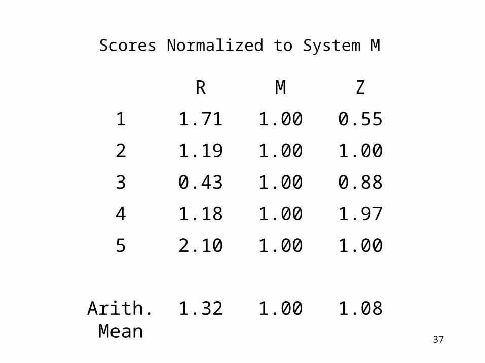
1.32 1.00 1.08

Scores Normalized to System M

38

Geometric Means

Geom. Mean of Scores Normalized Relative to R

Geom. Mean of Scores Normalized Relative to M

Similar situation if we test students on different benchmarks

R M Z

1.00 0.86 0.84

R M Z

1.17 1.00 0.99

39

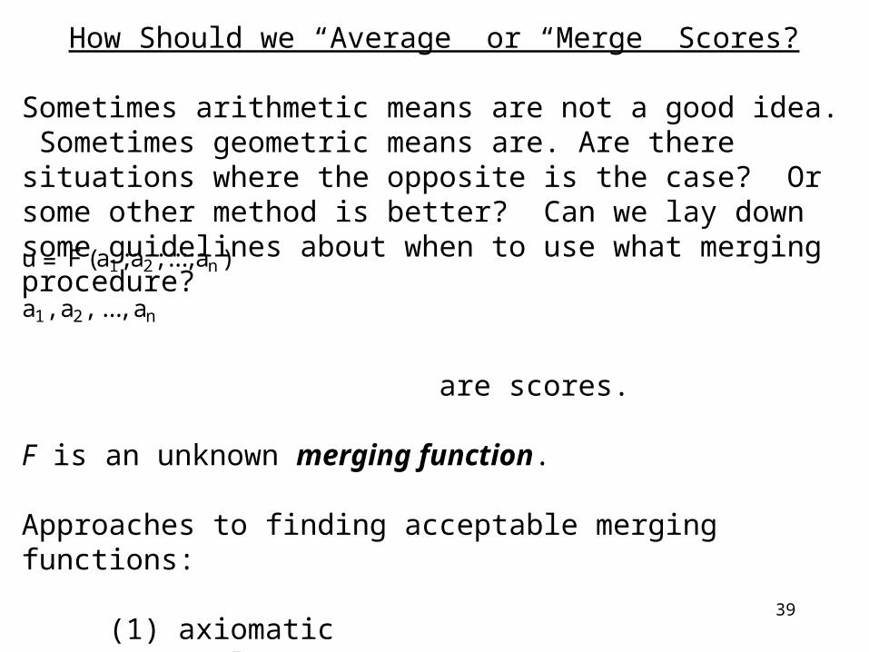
How Should we “Average” or “Merge” Scores?

Sometimes arithmetic means are not a good idea. Sometimes geometric means are. Are there situations where the opposite is the case? Or some other method is better? Can we lay down some guidelines about when to use what merging procedure?

are scores.

F is an unknown merging function.

Approaches to finding acceptable merging functions:

(1) axiomatic (2) scale types (3) meaningfulness

u= F (a1;a2; :::;an)

a1, a2, ..., an

40

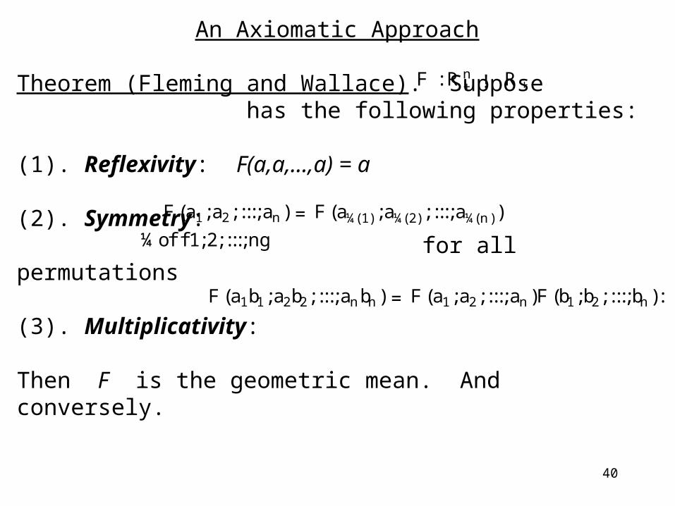
An Axiomatic Approach

Theorem (Fleming and Wallace). Suppose has the following properties:

(1). Reflexivity: F(a,a,...,a) = a

(2). Symmetry: for all permutations

(3). Multiplicativity:

Then F is the geometric mean. And conversely.

F : R n+ ! R+

F (a1;a2; :::;an) = F (a¼(1);a¼(2); :::;a¼(n))

¼of f1;2;:::;ng

F (a1b1;a2b2; :::;anbn) = F (a1;a2; :::;an)F (b1;b2; :::;bn):

41

A Functional Equations Approach Using Scale Type or Meaningfulness Assumptions

Unknown function

Luce's idea: If you know the scale types of the and the scale type of u and you assume that an admissible transformation of each of the leads to an admissible transformation of u, you can derive the form of F.

Example: are independent ratio scales, u is a ratio scale.

u= F (a1;a2; :::;an):

ai

ai

a1, a2, ..., an

F : R n+ ! R+

42

Thus, we get the functional equation:

(*)

Theorem (Luce 1964): If is continuous and satisfies (*), then there are so that

F (®1a1;®2a2; :::;®nan) =®u:

®1 >0, ®2 >0, ..., ®n >0, ®>0and ®depends on ®1, ®2, ..., ®n.

F (®1a1;®2a2; :::;®nan) =A(®1;®2; :::;®n)F (a1;a2; :::;an);

A(®1;®2; :::;®n) > 0

F : R n+¡ ! R+

¸ > 0, c1, c2, ..., cn

F (a1;a2; :::;an) = ¸ac11 ac22 :::a

cnn :

F (a1;a2; :::;an) = u !

43

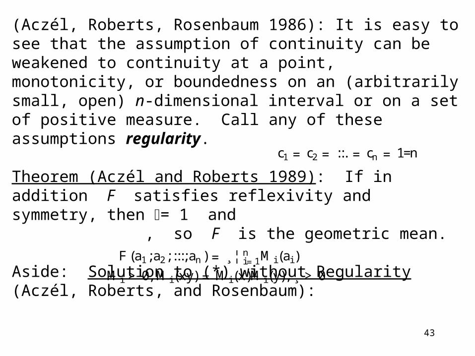
(Aczél, Roberts, Rosenbaum 1986): It is easy to see that the assumption of continuity can be weakened to continuity at a point, monotonicity, or boundedness on an (arbitrarily small, open) n-dimensional interval or on a set of positive measure. Call any of these assumptions regularity.

Theorem (Aczél and Roberts 1989): If in addition F satisfies reflexivity and symmetry, then = 1 and , so F is the geometric mean.

Aside: Solution to (*) without Regularity (Aczél, Roberts, and Rosenbaum):

c1 = c2 = ::. = cn =1=n

F (a1;a2; :::;an) = ¸¦ ni=1M i (ai )

M i >0, M i (xy) =M i (x)M i (y), ¸ > 0

44

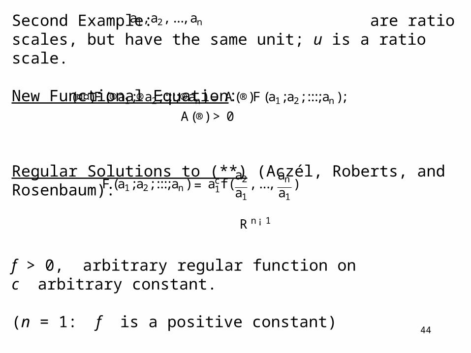
Second Example: are ratio scales, but have the same unit; u is a ratio scale.

New Functional Equation:

Regular Solutions to (**) (Aczél, Roberts, and Rosenbaum):

f > 0, arbitrary regular function onc arbitrary constant.

(n = 1: f is a positive constant)

a1, a2, ..., an

(¤¤)F (®a1;®a2; :::;®an) = A(®)F (a1;a2; :::;an);

A(®) > 0

F (a1;a2; :::;an) = ac1f (a2a1, ...,

ana1)

R n¡ 1

45

Solutions to (**) without Regularity (Aczél, Roberts, and Rosenbaum):

Third Example: are independent ratio scales, u is an interval scale

New Functional Equation:

(***)

F (a1;a2; :::;an) =M (a1)f (a2a1, ...,

ana1)

f > 0, arbitrary function

M > 0, M (xy) =M (x)M (y):

a1, a2, ..., an

F (®1a1;®2a2; :::;®nan) =A(®1;®2; :::;®n)F (a1;a2; :::;an)+

B(®1;®2; :::;®n);

A(®1;®2; :::;®n) > 0

46

Regular solutions to (***) (Aczél, Roberts, and Rosenbaum):

OR

F (a1;a2; :::;an) = ¸¦ ni=1a

ci i +b

¸, b, c1, c2, ..., cn arbitrary constants

F (a1;a2; :::;an) =nX

i=1

ci logai +b

b, c1, c2, ..., cn arbitrary constants.

47

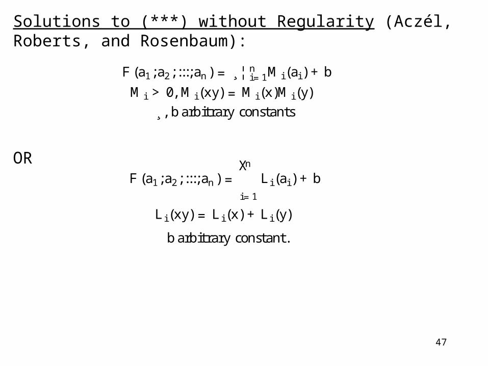
Solutions to (***) without Regularity (Aczél, Roberts, and Rosenbaum):

OR

F (a1;a2; :::;an) = ¸¦ ni=1M i (ai ) +b

M i >0, M i (xy) =M i (x)M i (y)¸, barbitrary constants

F (a1;a2; :::;an) =nX

i=1

L i (ai ) +b

L i (xy) = L i (x) +L i (y)

barbitrary constant.

48

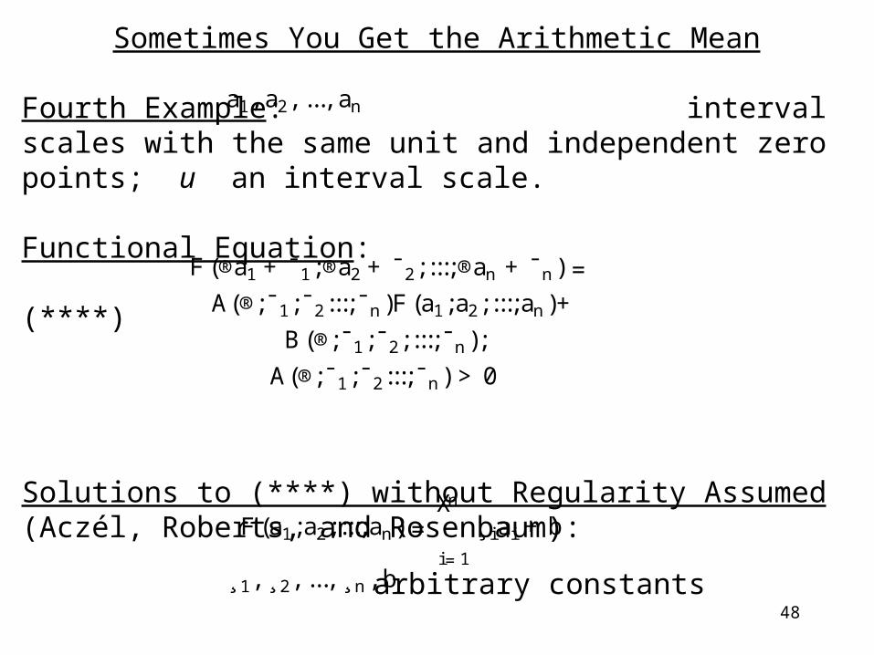
Sometimes You Get the Arithmetic Mean

Fourth Example: interval scales with the same unit and independent zero points; u an interval scale.

Functional Equation:

(****)

Solutions to (****) without Regularity Assumed (Aczél, Roberts, and Rosenbaum):

a1, a2, ..., an

F (®a1+¯1;®a2+¯2; :::;®an +¯n) =A(®;¯1;¯2:::;¯n)F (a1;a2; :::;an)+

B(®;¯1;¯2; :::;¯n);

A(®;¯1;¯2:::;¯n) > 0

F (a1;a2; :::;an) =nX

i=1

¸ iai +b

¸1, ¸2, ..., ¸n , b arbitrary constants

49

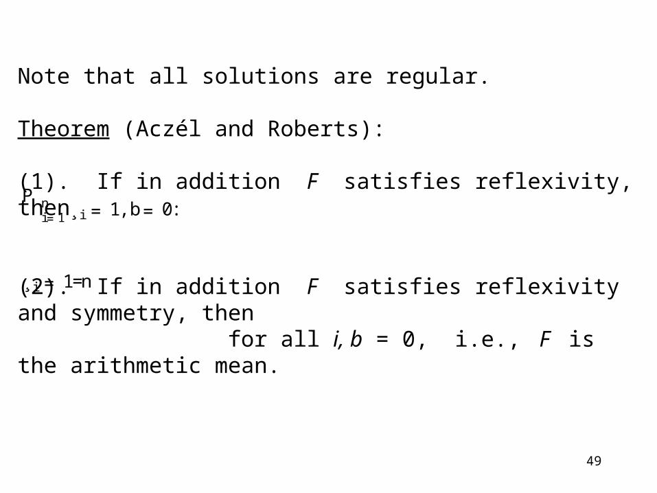
Note that all solutions are regular.

Theorem (Aczél and Roberts):

(1). If in addition F satisfies reflexivity, then

(2). If in addition F satisfies reflexivity and symmetry, then for all i, b = 0, i.e., F is the arithmetic mean.

P ni=1

¸ i =1, b= 0:

¸ i =1=n

50

Meaningfulness Approach

While it is often reasonable to assume you know the scale type of the independent variables , it is not so often reasonable to assume that you know the scale type of the dependent variable u. However, it turns out that you can replace the assumption that the scale type of u is xxxxxxx by the assumption that a certain statement involving u is meaningful.

a1, a2, ..., an

51

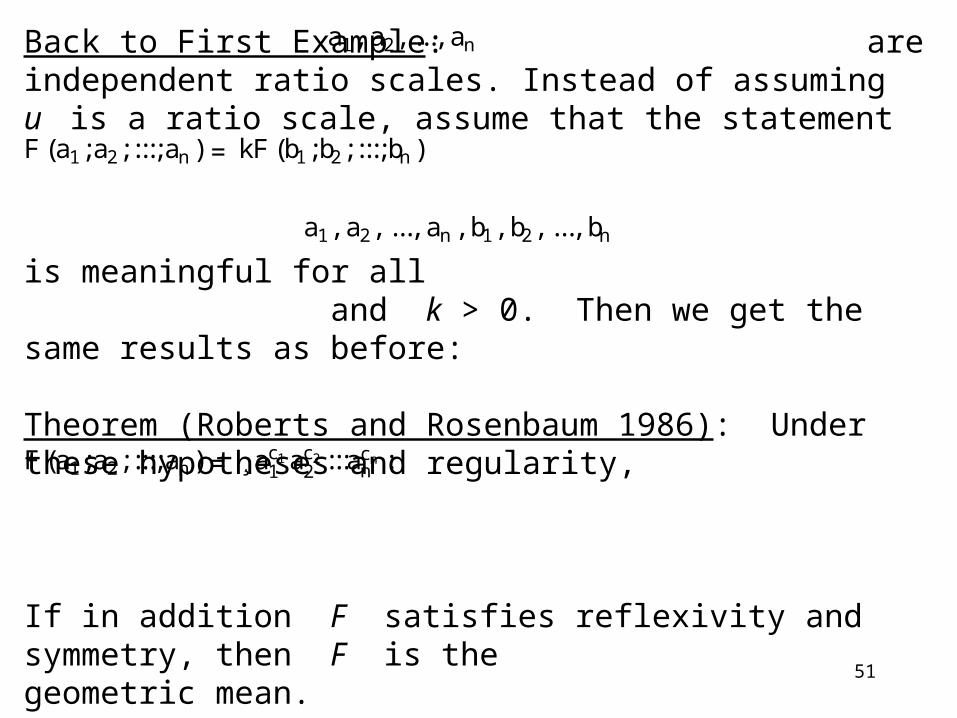
Back to First Example: are independent ratio scales. Instead of assuming u is a ratio scale, assume that the statement

is meaningful for all and k > 0. Then we get the same results as before:

Theorem (Roberts and Rosenbaum 1986): Under these hypotheses and regularity,

If in addition F satisfies reflexivity and symmetry, then F is the geometric mean.

a1, a2, ..., an

F (a1;a2; :::;an) = kF (b1;b2; :::;bn)

a1, a2, ..., an , b1, b2, ..., bn

F (a1;a2; :::;an) = ¸ac11 ac22 :::a

cnn :

52

MEASUREMENT OF AIR POLLUTION

Various pollutants are present in the air:

Carbon monoxide (CO), hydrocarbons (HC), nitrogen oxides (NOX), sulfur oxides (SOX), particulate matter (PM).

Also damaging: Products of chemical reactions among pollutants. E.g.: Oxidants such as ozone produced by HC and NOX reacting in presence of sunlight.

Some pollutants are more serious in presence of others, e.g., SOX are more harmful in presence of PM.

Can we measure pollution with one overall measure?

53

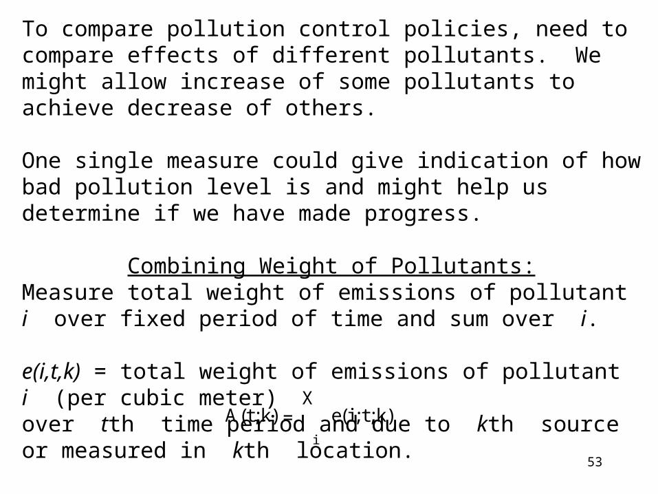
To compare pollution control policies, need to compare effects of different pollutants. We might allow increase of some pollutants to achieve decrease of others.

One single measure could give indication of how bad pollution level is and might help us determine if we have made progress.

Combining Weight of Pollutants:Measure total weight of emissions of pollutant i over fixed period of time and sum over i.

e(i,t,k) = total weight of emissions of pollutant i (per cubic meter) over tth time period and due to kth source or measured in kth location.

A(t;k) =X

i

e(i;t;k)

54

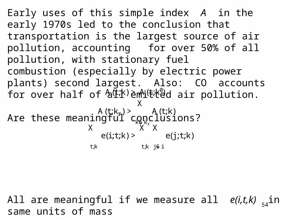
Early uses of this simple index A in the early 1970s led to the conclusion that transportation is the largest source of air pollution, accounting for over 50% of all pollution, with stationary fuel combustion (especially by electric power plants) second largest. Also: CO accounts for over half of all emitted air pollution.

Are these meaningful conclusions?

All are meaningful if we measure all e(i,t,k) in same units of mass (e.g., milligrams per cubic meter) and so admissible transformation means multiply e(i,t,k) by same constant.

A(t;k) > A(t;k0)

A(t;kr ) >X

k6=kr

A(t;k)

X

t;k

e(i;t;k) >X

t;k

X

j 6=i

e(j ;t;k)

55

These comparisons are meaningful in the technical sense.

But: Are they meaningful comparisons of pollution level in a practical sense?

A unit of mass of CO is far less harmful than a unit of mass of NOX. EPA standards based on health effects for 24 hour period allow 7800 units of CO to 330 units of NOX. These are Minimum acute toxicity effluent tolerance factors (MATE criteria).

Tolerance factor is level at which adverse effects are known. Let t(i) be tolerance factor for ith pollutant.

Severity factor: t(CO)/t(i) or 1/t(i)

56

One idea (Babcock and Nagda, Walther, Caretto and Sawyer): Weight the emission levels (in mass) by severity factor and get a weighted sum. This amounts to using the indices

Degree of hazard:

and the combined index

Pindex:

Under pindex, transportation is still the largest source of pollutants, but now accounting for less than 50%. Stationary sources fall to fourth place. CO drops to bottom of list of pollutants, accounting for just over 2% of the total.

1t(i )e(i;t;k)

B(t;k) =P

i1t(i )e(i;t;k)

57

These conclusions are again meaningful if all emission weights are measured in same units. For an admissible transformation multiplies t and e by the same constant and thus leaves the degree of hazard unchanged and pindex unchanged.

Pindex was introduced in the San Francisco Bay Area in the 1960s.

But, are comparisons using pindex meaningful in the practical sense?

Pindex amounts to: for a given pollutant, take the percentage of a given harmful level of emissions that is reached in a given period of time, and add up these percentages over all pollutants. (Sum can be greater than 100% as a result.)

58

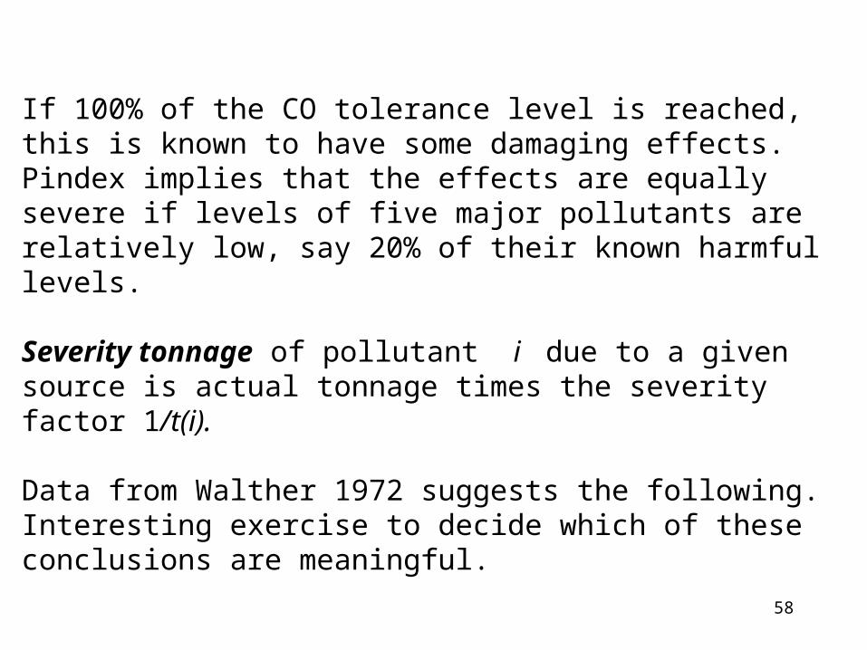
If 100% of the CO tolerance level is reached, this is known to have some damaging effects. Pindex implies that the effects are equally severe if levels of five major pollutants are relatively low, say 20% of their known harmful levels.

Severity tonnage of pollutant i due to a given source is actual tonnage times the severity factor 1/t(i).

Data from Walther 1972 suggests the following. Interesting exercise to decide which of these conclusions are meaningful.

59

1. HC emissions are more severe (have greater severity tonnage) than NOX emissions.

2. Effects of HC emissions from transportation are more severe than those of HC emissions from industry. (Same for NOX.).

3. Effects of HC emissions from transportation are more severe than those of CO emissions from industry.

4. Effects of HC emissions from transportation are more than 20 times as severe as effects of CO emissions from transportation.

5. The total effect of HC emissions due to all sources is more than 8 times as severe as total effect of NOX emissions due to all sources.

60

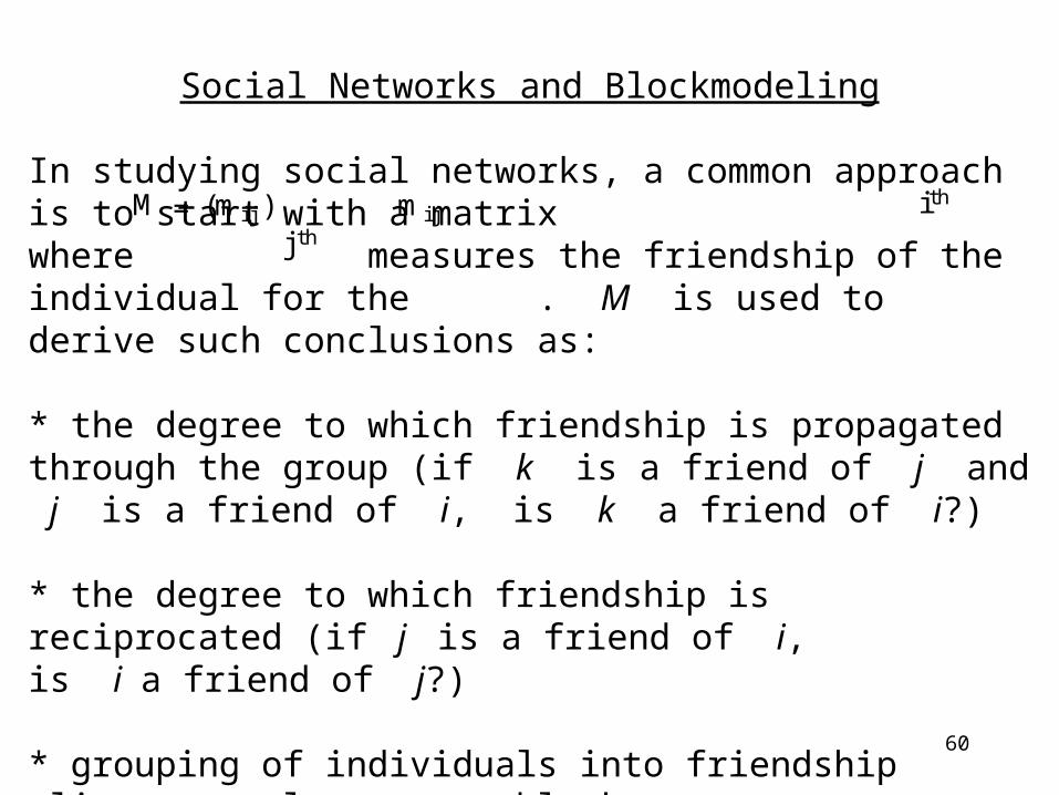
Social Networks and Blockmodeling

In studying social networks, a common approach is to start with a matrix where measures the friendship of the individual for the . M is used to derive such conclusions as:

* the degree to which friendship is propagated through the group (if k is a friend of j and j is a friend of i, is k a friend of i?)

* the degree to which friendship is reciprocated (if j is a friend of i, is i a friend of j?)

* grouping of individuals into friendship cliques or clusters or blocks.

M = (mi j ) mi j ith

j th

61

Batchelder: Unless attention is paid to the types of scales used to measure , conclusions about propagation, reciprocation, and grouping can be meaningless.

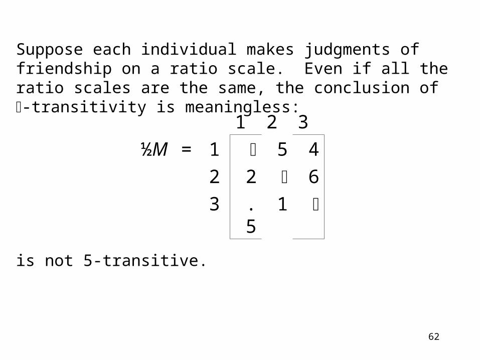
Simple Example: -Transitivity

The social network is called -transitive ( > 0) if

is 5-transitive.

mi j

1 2 3

M = 1 10 8

2 4 12

3 1 2

[mi j ¸ ±]&[mj k ¸ ±] ! mik ¸ ±, i 6= k:

62

Suppose each individual makes judgments of friendship on a ratio scale. Even if all the ratio scales are the same, the conclusion of -transitivity is meaningless:

is not 5-transitive.

1 2 3

½M

= 1 5 4

2 2 6

3 .5 1

63

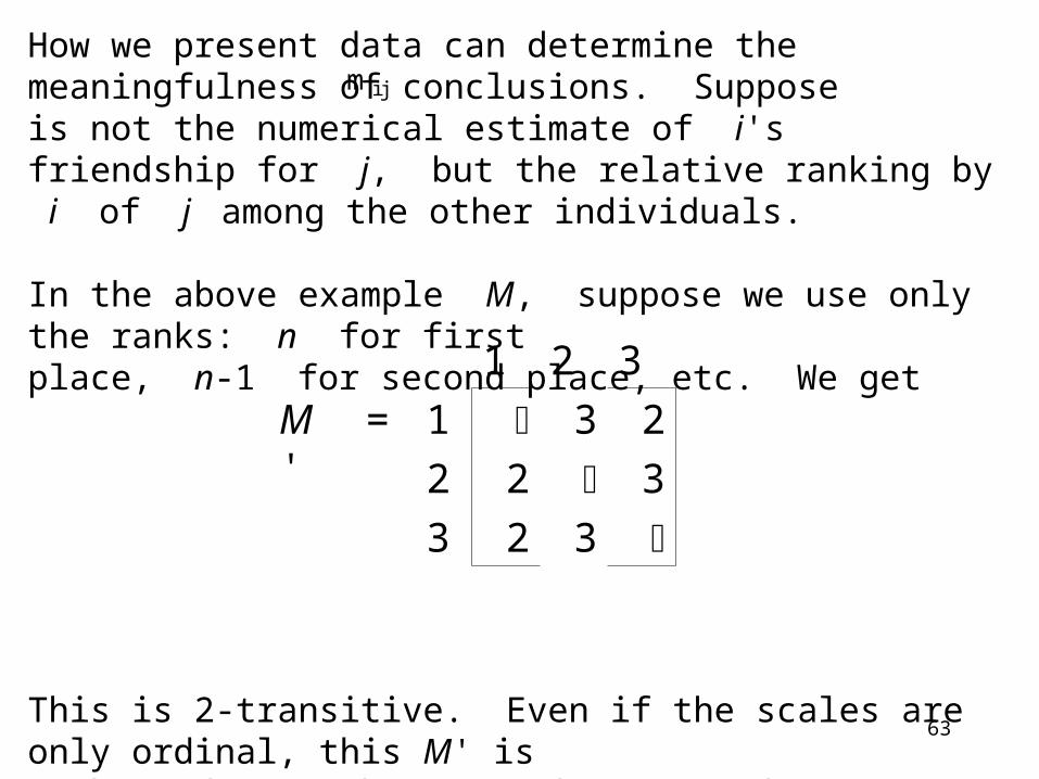
How we present data can determine the meaningfulness of conclusions. Suppose is not the numerical estimate of i's friendship for j, but the relative ranking by i of j among the other individuals.

In the above example M, suppose we use only the ranks: n for first place, n-1 for second place, etc. We get

This is 2-transitive. Even if the scales are only ordinal, this M' is unchanged even when M changes. Thus, -transitivity of M' is a meaningful conclusion. (Batchelder)

mi j

1 2 3

M ' = 1 3 2

2 2 3

3 2 3

64

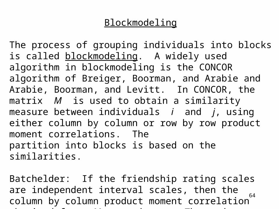
Blockmodeling

The process of grouping individuals into blocks is called blockmodeling. A widely used algorithm in blockmodeling is the CONCOR algorithm of Breiger, Boorman, and Arabie and Arabie, Boorman, and Levitt. In CONCOR, the matrix M is used to obtain a similarity measure between individuals i and j, using either column by column or row by row product moment correlations. The partition into blocks is based on the similarities.

Batchelder: If the friendship rating scales are independent interval scales, then the column by column product moment correlation obtained from M can change. Thus, the blocks can also change.

65

Hence, the blocking conclusions from a procedure such as CONCOR can be meaningless.

E.g.: Suppose is the Pearson column by column product moment correlation obtained from matrix M and suppose is the same correlation obtained from M', where

If , , , then and . This is as dramatic a change as possible.

ci jc0i j

m0i j =®imi j +¯ i , ®i >0:

®1 =®2 =®3 =1 ®4 =3 ¯1 = ¯2 = ¯3 = ¯4 =0 c12 =1c012 = ¡ 1

0 2 2 1

2 0 6 3

Let M = 2 4 0 5

1 1 3 0

66

Note: Batchelder shows that if is the product moment correlation between the and rows of M, then under the transformation

is invariant. Thus, conclusions from M based on row by row correlations are meaningful.

ri j

ith j th

m0i j =®imi j +¯ i , ®i >0;

ri j

67

Meaningfulness of Statistical Tests(Marcus-Roberts and Roberts)

For more than 40 years, there has been considerable disagreement on the limitations that scales of measurement impose on statistical procedures we may apply. The controversy stems from the foundational work of Stevens (1946, 1951, 1959, ...), who developed the classification of scales of measurement we have given and then provided rules for the use of statistical procedures which provided that certain statistics were inappropriate at certain levels of measurement. The application of Stevens' ideas to descriptive statistics has been widely accepted, but the application to inferential statistics has been labeled by some a misconception.

68

Descriptive Statistics

P = population whose distribution we would like to describe

We try to capture some of the properties of P by finding some descriptive statistic for P or by taking a sample S from P and finding a descriptive statistic for S.

Our previous examples suggest that certain descriptive statistics are appropriate only for certain measurement situations. This idea was originally due to Stevens and was popularized by Siegel in his well-known book Nonparametric Statistics (1956).

69

Our examples suggest the principle that arithmetic means are “appropriate” statistics for interval scales, medians for ordinal scales.

The other side of the coin: It is argued that it is always appropriate to calculate means, medians, and other descriptive statistics, no matter what the scale of measurement.

Frederic Lord: Famous football player example. “The numbers don't remember where they came from.”

I agree: It is always appropriate to calculate means, medians, ...But: Is it appropriate to make certain statements using these descriptive statistics?

70

My position: It is usually appropriate to make a statement using descriptive statistics if and only if the statement is meaningful. Why? A statement which is true but meaningless gives information which is an accident of the scale of measurement used, not information which describes the population in some fundamental way.

So, it is appropriate to calculate the mean of ordinal data, it is just not appropriate to say that the mean of one group is higher than the mean of another group.

71

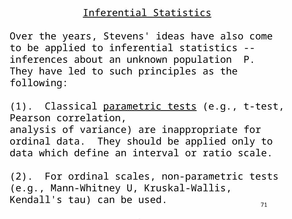
Inferential Statistics

Over the years, Stevens' ideas have also come to be applied to inferential statistics -- inferences about an unknown population P. They have led to such principles as the following:

(1). Classical parametric tests (e.g., t-test, Pearson correlation, analysis of variance) are inappropriate for ordinal data. They should be applied only to data which define an interval or ratio scale.

(2). For ordinal scales, non-parametric tests (e.g., Mann-Whitney U, Kruskal-Wallis, Kendall's tau) can be used.

Not everyone agrees. Thus: Controversy

72

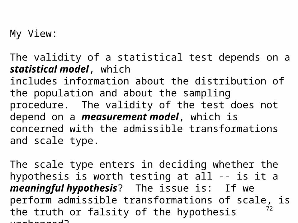
My View:

The validity of a statistical test depends on a statistical model, which includes information about the distribution of the population and about the sampling procedure. The validity of the test does not depend on a measurement model, which is concerned with the admissible transformations and scale type.

The scale type enters in deciding whether the hypothesis is worth testing at all -- is it a meaningful hypothesis? The issue is: If we perform admissible transformations of scale, is the truth or falsity of the hypothesis unchanged?

73

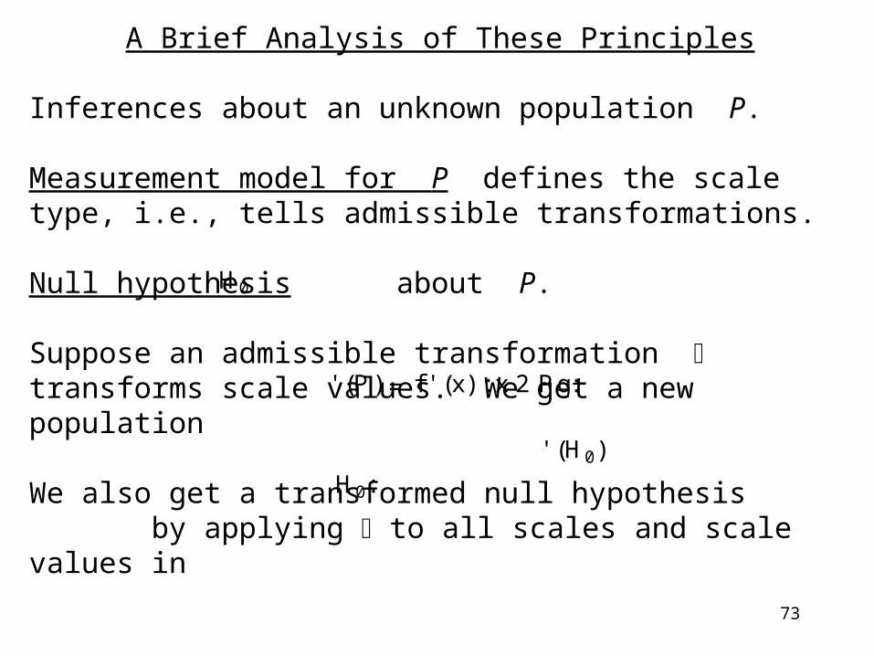
A Brief Analysis of These Principles

Inferences about an unknown population P.

Measurement model for P defines the scale type, i.e., tells admissible transformations.

Null hypothesis about P.

Suppose an admissible transformation transforms scale values. We get a new population

We also get a transformed null hypothesis by applying to all scales and scale values in

H0

' (P ) = f ' (x) : x 2 Pg:

' (H0)H0:

74

Example: mean of P is 0.

Measurement model: P ordinal Then is admissible. mean of (P) is

Note that if , then is true.

Also, and so is false.

Thus, a null hypothesis can be meaningless.

Summary of my position: The major restriction measurement theory places on inferential statistics is on what hypotheses are meaningful. We should be primarily concerned with testing meaningful hypotheses.

H0 :

' (x) = ex

' (H0) : ' (0) = e0 =1:

P = f ¡ 2, -1, 0, 1, 2g H0

' (P ) = fe¡ 2, e¡ 1, e0, e1, e2g ' (H0)

75

Can we test meaningless hypotheses? Sure. But I question what information we get outside of information about the population as measured.

More details: Testing about P :

1). Draw a random sample S from P.2). Calculate a test statistic based on S.3). Calculate probability that the test statistic is what was observed given is true.4). Accept or reject on the basis of the test.

Note: Calculation of probability depends on a statistical model, which includes information about the distribution of P and about the sampling procedure. But, the validity of the test depends only on the statistical model, not on the measurement model.

H0

H0

H0

76

Thus, you can apply parametric tests to ordinal data, provided the statistical model is satisfied, in particular if the data is normally distributed. (Thomas showed that ordinal data can be normallydistributed; it is a misconception that it cannot be.)

Where does the scale type enter? In determining if the hypothesis is worth testing at all. i.e., if it is meaningful.

For instance, consider ordinal data and

The hypothesis is meaningless. But, if the data meets certain distributional requirements such as normality, we can apply a parametric test, such as the t-test, to check if the mean is 0.

H0 : Themean is 0.

77

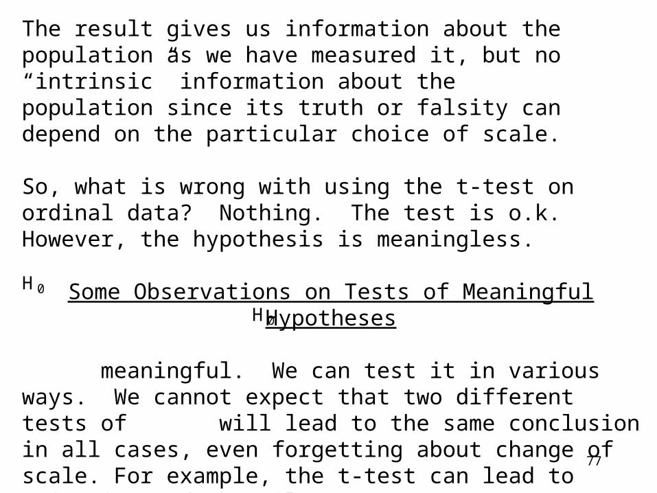
The result gives us information about the population as we have measured it, but no “intrinsic” information about the population since its truth or falsity can depend on the particular choice of scale.

So, what is wrong with using the t-test on ordinal data? Nothing. The test is o.k. However, the hypothesis is meaningless.

Some Observations on Tests of Meaningful Hypotheses

meaningful. We can test it in various ways. We cannot expect that two different tests of will lead to the same conclusion in all cases, even forgetting about change of scale. For example, the t-test can lead to rejection and the Wilcoxon test to acceptance.

H0

H0

78

But what happens if we apply the same test to data both before and after admissible transformation? The best situation is if the results of the test are invariant under admissible changes of scale. More precisely: Suppose is a meaningful hypothesis about population P. Test by drawing a random sample S from P. Let (S) be the set of all (x) for x in S. We hope for a test T for with the following properties:

(a). The statistical model for T is satisfied by P and also by (P) for all admissible transformations as defined by the measurement model for P.

(b) T accepts with sample S at level of significance if and only if T accepts with sample (S) at level of significance .

H0

H0

H0

H0

' (H0)

79

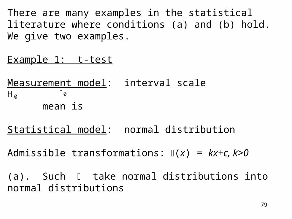
There are many examples in the statistical literature where conditions (a) and (b) hold. We give two examples.

Example 1: t-test

Measurement model: interval scale

mean is

Statistical model: normal distribution

Admissible transformations: (x) = kx+c, k>0

(a). Such take normal distributions into normal distributions

H0¹ 0

80

(b) The test statistic is

where n = sample size, = sample mean, = sample variance.

Transform by (x) = kx+c.

New sample mean is ; new sample variance is

mean is

New test statistic for

The test statistic is the same, so (b) follows.

s2

k2s2:

' (H0) : ' (¹ 0) = k¹ 0+c:

' (H0) :

t = [X ¡ ¹ 0]=(s=pn)

X

kX +c

[kX +c¡ (k¹ 0+c)]=(ks=pn) = t:

81

Example 2: Sign Test

Measurement model: ordinal scale

median is (meaningful)

Statistical model: Literature of nonparametric statistics is unclear. Most books say continuity of probability density function is needed. In fact, it is only necessary to assume

.

(a)

( is strictly increasing)

(Note that strictly increasing also take continuous data into continuous data, since there are only countably many gaps)

H0 : M0

P r(x =M0) = 0

P r(x =M0) = 0$ P r(' (x) = ' (M0)) = 0

82

(b) Test statistic: Number of sample points above or number below , whichever is smaller. This test statistic does not change when a strictly increasing is applied to S and is replaced by . Thus, (b) follows.

What if Conditions (a) or (b) Fail?

What if (a) holds, (b) fails?

We might still find test T useful, just as we sometimes find it useful to apply different tests with possibly different conclusions to the same data. However, it is a little disturbing that seemingly innocuous changes in how we measure things could lead to different conclusions under the “same” test.

M0

M0

M0

' (M0)

83

What if is meaningful but (a) fails?

This could happen if P violates the statistical model for T. We might still be able to test using T: Try to find admissible such that satisfies the statistical model for T and then apply T to test . Since is meaningful, holds iff , so T applied to gives a test for .

For instance, if is meaningful, then even for ordinal data, we can seek a transformation which normalizes the data and allows us to apply a parametric test.

H0

' (P )H0 H0

' (P ) H0

H0

H0

' (H0)' (H0)

84

What if conditions (a) or (b) fail and we still apply test T to test ?

There is much empirical work on this, especially emphasizing the situation where (a) and (b) fail because we have an ordinal scale but we treat it like an interval scale. I don't think measurement theory has much to say about this situation. But good theoretical work does, and more is needed.

H0

85

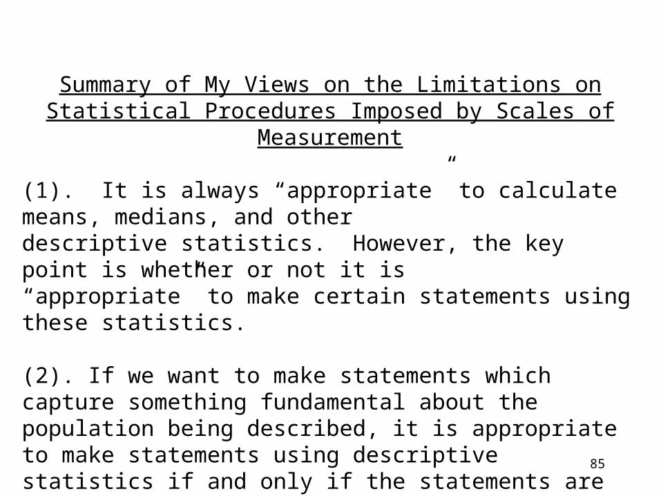
Summary of My Views on the Limitations on Statistical Procedures Imposed by Scales of Measurement

(1). It is always “appropriate” to calculate means, medians, and other descriptive statistics. However, the key point is whether or not it is “appropriate” to make certain statements using these statistics.

(2). If we want to make statements which capture something fundamental about the population being described, it is appropriate to make statements using descriptive statistics if and only if the statements are meaningful.

86

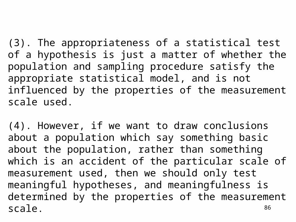
(3). The appropriateness of a statistical test of a hypothesis is just a matter of whether the population and sampling procedure satisfy the appropriate statistical model, and is not influenced by the properties of the measurement scale used.

(4). However, if we want to draw conclusions about a population which say something basic about the population, rather than something which is an accident of the particular scale of measurement used, then we should only test meaningful hypotheses, and meaningfulness is determined by the properties of the measurement scale.

87

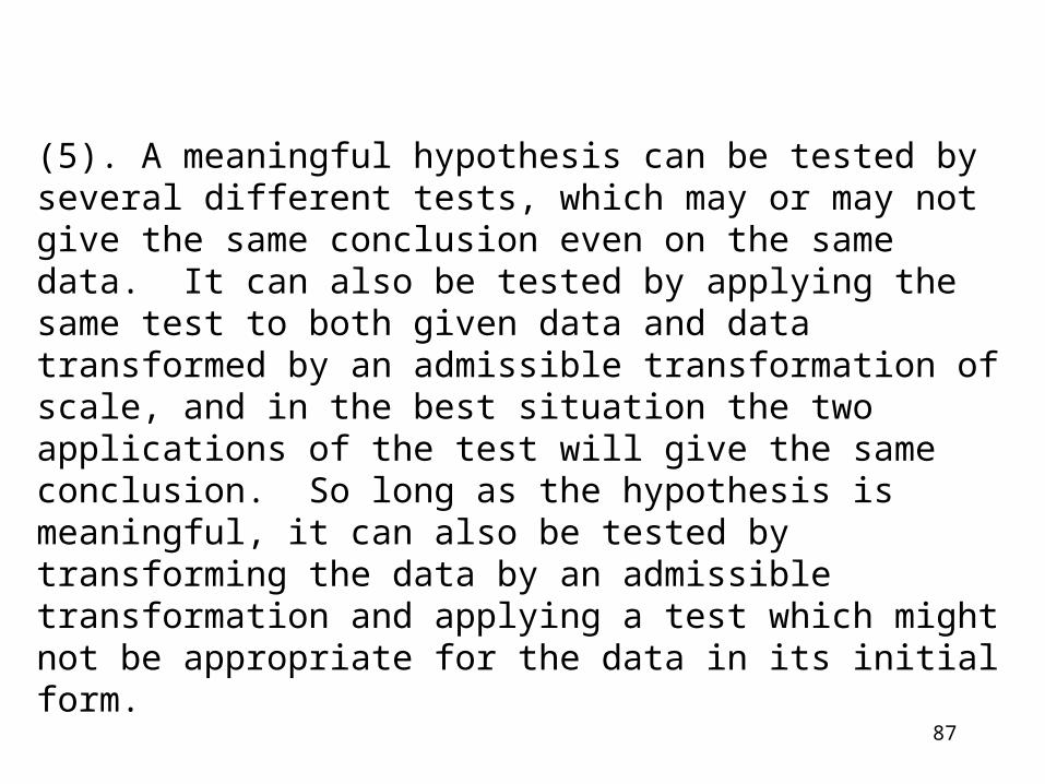
(5). A meaningful hypothesis can be tested by several different tests, which may or may not give the same conclusion even on the samedata. It can also be tested by applying the same test to both given data and data transformed by an admissible transformation of scale, and in the best situation the two applications of the test will give the same conclusion. So long as the hypothesis is meaningful, it can also be tested by transforming the data by an admissible transformation and applying a test which might not be appropriate for the data in its initial form.

88

The First Representation Problem: Ordinal Utility Functions

Homomorphism from (A,R) into

R = warmer than, louder than, preferred to, ...

If preference, then f is an ordinal utility function.

Definition: We say that (A,R) is a strict weak order if it satisfies the following two conditions:

(1). Asymmetry: aRb ~bra

(2). Negative Transitivity: ~aRb & ~bRc ~aRc

(R ;>):f : A ! RaRb$ f (a) > f (b)

!

!

89

Example:

aRb a is to the right of b

Representation Theorem: Suppose A is a finite set. Then (A,R) is homomorphic to iff (A,R) is a strict weak order.

This says that our example with the 's is the most general strict weak order on a finite set.

(R ;>)

$

90

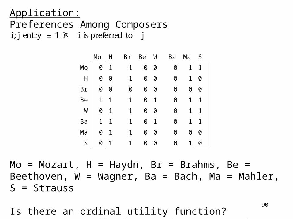
Application:Preferences Among Composers

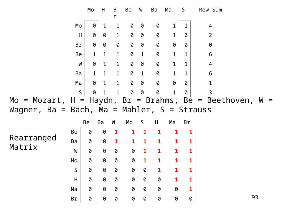
Mo = Mozart, H = Haydn, Br = Brahms, Be = Beethoven, W = Wagner, Ba = Bach, Ma = Mahler, S = Strauss

Is there an ordinal utility function?How does one tell if (A,R) is strict weak?

i; j entry = 1 i® i is preferred to j

Mo H Br Be W Ba Ma S

Mo 0 1 1 0 0 0 1 1

H 0 0 1 0 0 0 1 0

Br 0 0 0 0 0 0 0 0

Be 1 1 1 0 1 0 1 1

W 0 1 1 0 0 0 1 1

Ba 1 1 1 0 1 0 1 1

Ma 0 1 1 0 0 0 0 0

S 0 1 1 0 0 0 1 0

91

Proof of the Representation Theorem for A Finite:

Necessity: straightforward

Sufficiency:

If (A,R) is strict weak, then f is a homomorphism.

Suppose aRb. Then ~bRa. Hence, ~aRy implies ~bRy, i.e., bRy implies aRy. It follows that f(a) f(b). By asymmetry, ~bRb. Since aRb, it follows that f(a) > f(b).

Suppose ~aRb. Then ~bRy implies ~aRy, so aRy implies bRy, sof(b) f(a), i.e., ~f(a) > f(b).

Let f (x) = jfy : xRygj:

¸

¸

92

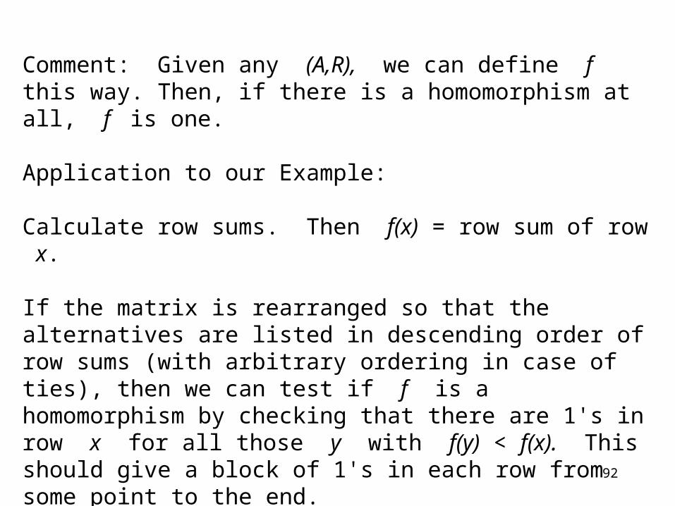
Comment: Given any (A,R), we can define f this way. Then, if there is a homomorphism at all, f is one.

Application to our Example:

Calculate row sums. Then f(x) = row sum of row x.

If the matrix is rearranged so that the alternatives are listed in descending order of row sums (with arbitrary ordering in case of ties), then we can test if f is a homomorphism by checking that there are 1's in row x for all those y with f(y) < f(x). This should give a block of 1's in each row from some point to the end.

93

Mo = Mozart, H = Haydn, Br = Brahms, Be = Beethoven, W = Wagner, Ba = Bach, Ma = Mahler, S = Strauss

RearrangedMatrix

Mo H Br Be W Ba Ma S Row Sum

Mo 0 1 1 0 0 0 1 1 4

H 0 0 1 0 0 0 1 0 2

Br 0 0 0 0 0 0 0 0 0

Be 1 1 1 0 1 0 1 1 6

W 0 1 1 0 0 0 1 1 4

Ba 1 1 1 0 1 0 1 1 6

Ma 0 1 1 0 0 0 0 0 1

S 0 1 1 0 0 0 1 0 3

Be Ba W Mo S H Ma Br

Be 0 0 1 1 1 1 1 1

Ba 0 0 1 1 1 1 1 1

W 0 0 0 0 1 1 1 1

Mo 0 0 0 0 1 1 1 1

S 0 0 0 0 0 1 1 1

H 0 0 0 0 0 0 1 1

Ma 0 0 0 0 0 0 0 1

Br 0 0 0 0 0 0 0 0

94

Are the axioms reasonable?Prescriptive vs. descriptive.As descriptive axioms for warmer than or preferred to:

Asymmetry: Seems ok for both.

Negative transitivity: Seems ok for warmer than. However, for preference, consider the following case. We choose on the basis of price, unless prices are close, in which case we choose by quality. Suppose a is higher quality than b, which is higher quality than c, with a higher in price than b and b higher in price than c. If a and b are close in price and so are b and c, but a and c are not, then we would choose a over b and b over c, but c over a. Thus, ~cRb and ~bRa, but cRa.

95

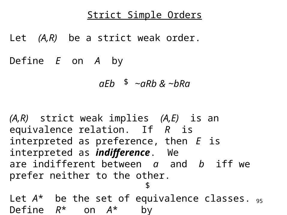
Strict Simple Orders

Let (A,R) be a strict weak order.

Define E on A by

aEb ~aRb & ~bRa

(A,R) strict weak implies (A,E) is an equivalence relation. If R isinterpreted as preference, then E is interpreted as indifference. Weare indifferent between a and b iff we prefer neither to the other.

Let A* be the set of equivalence classes. Define R* on A* by

aR*b* aRb

$

$

96

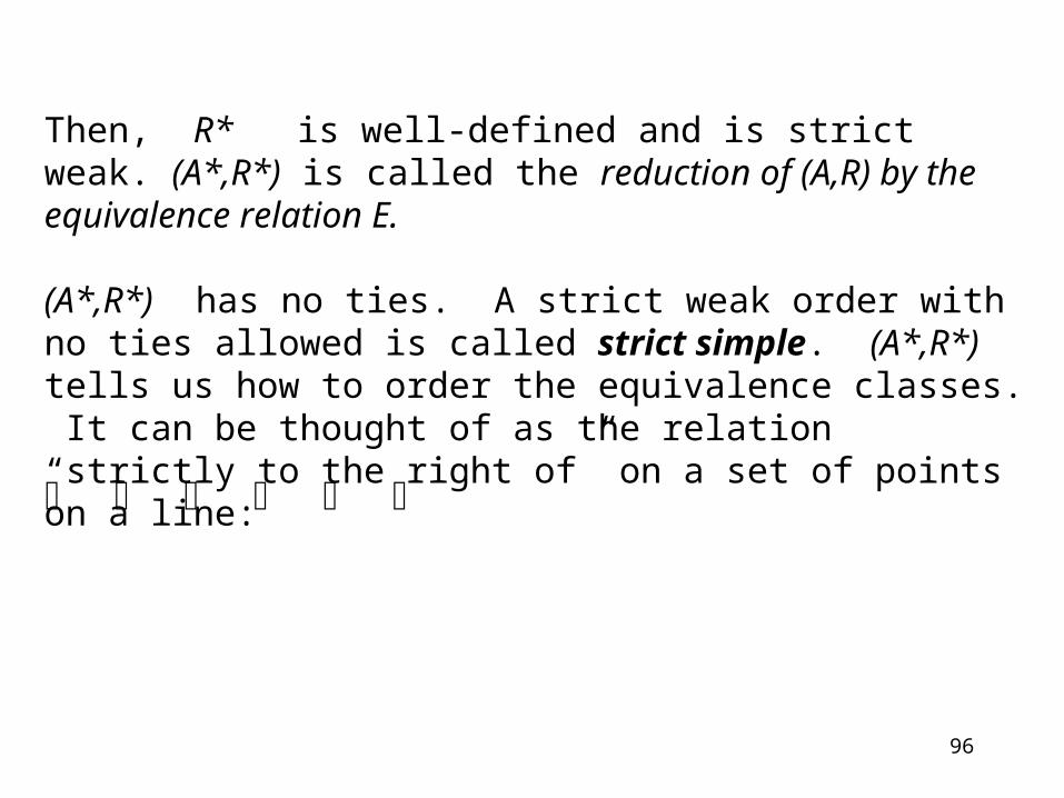
Then, R* is well-defined and is strict weak. (A*,R*) is called the reduction of (A,R) by the equivalence relation E.

(A*,R*) has no ties. A strict weak order with no ties allowed is called strict simple. (A*,R*) tells us how to order the equivalence classes. It can be thought of as the relation “strictly to the right of” on a set of points on a line:

97

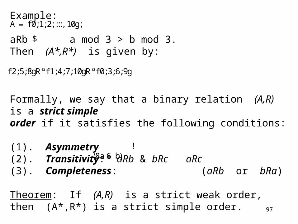
Example:

aRb a mod 3 > b mod 3.Then (A*,R*) is given by:

Formally, we say that a binary relation (A,R) is a strict simple order if it satisfies the following conditions:

(1). Asymmetry(2). Transitivity: aRb & bRc aRc (3). Completeness: (aRb or bRa)

Theorem: If (A,R) is a strict weak order, then (A*,R*) is a strict simple order.

A = f0;1;2;:::, 10g;

f2;5;8gR¤f1;4;7;10gR¤f0;3;6;9g

(8a 6= b)

$

!

98

Theorem: If A is a finite set, then there is a 1-1 homomorphism from (A,R) into iff (A,R) is a strict simple order.

Weak Orders

is not a strict simple order. It violates asymmetry: We can have aRb and bRa. Similarly, “weakly to the right of” on a set of points is not a strict weak order for the same reason.

(R ;>)

(R ;¸ )

99

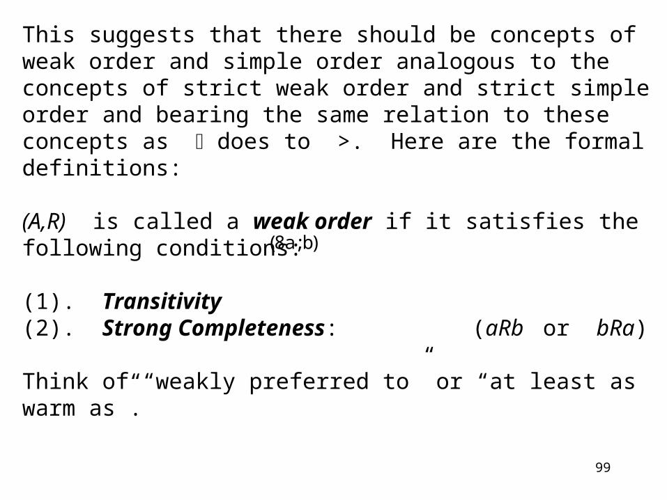
This suggests that there should be concepts of weak order and simple order analogous to the concepts of strict weak order and strict simple order and bearing the same relation to these concepts as does to >. Here are the formal definitions:

(A,R) is called a weak order if it satisfies the following conditions:

(1). Transitivity(2). Strong Completeness: (aRb or bRa)

Think of “weakly preferred to” or “at least as warm as”.

(8a;b)

100

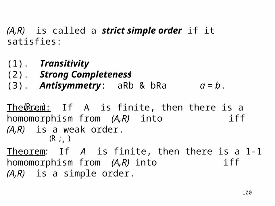
(A,R) is called a strict simple order if it satisfies:

(1). Transitivity(2). Strong Completeness(3). Antisymmetry: aRb & bRa a = b. Theorem: If A is finite, then there is a homomorphism from (A,R) into iff (A,R) is a weak order.

Theorem: If A is finite, then there is a 1-1 homomorphism from (A,R) into iff (A,R) is a simple order.

(R ;¸ )

(R ;¸ )

!

101

If (A,R) is a weak order, define a binary relation E on A by:

aEb aRb & bRa

Then (A,E) is an equivalence relation. Again, we can define a binary relation R* on the set A* of equivalence classes, with

a*R*b* aRb

hen (A*,R*) is well-defined and is a simple order.

$

$

102

Generalizations of the Representation Theorem to Infinite Sets of Alternatives.

Cantor's Theorem (1895): If A is a countable set, then (A,R) is homomorphic to iff (A,R) is a strict weak order.

This theorem fails for arbitrary infinite sets.Use the lexicographic ordering of the plane:

This is strict weak, but there is no homomorphism:f(a,1) > f(a,0). rational number g(a) with f(a,1) > g(a) > f(a,0).g is 1-1 function from reals into rationals:

a > b g(a) > f(a,0) > f(b,1) > g(b)

(R ;>)

A =R £ R(a;b)R(s;t) $ [a> s or (a= s&b> t)]:

!

103

Birkhoff-Milgram Theorem

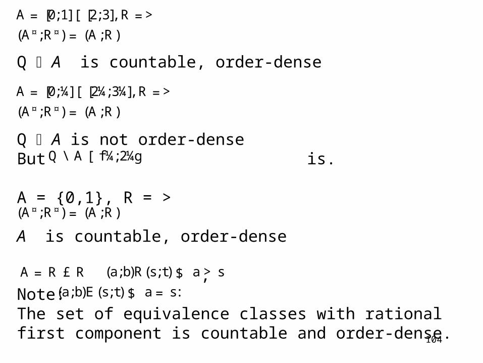
(A,R) binary relation, B A.

Say B is order-dense in A if a,b A-B, aRb and ~bRa implythat c B such that aRcRb.

Theorem (Birkhoff-Milgram): (A,R) is homomorphic to iff (A,R) is a strict weak order and has a countable set which is order-dense.

(R ;>)

(A¤;R¤)

104

Q A is countable, order-dense

Q A is not order-denseBut is.

A = {0,1}, R = >

A is countable, order-dense

, Note:The set of equivalence classes with rational first component is countable and order-dense.

A = [0;1][ [2;3], R =>

(A¤;R¤) = (A;R)

A = [0;¼][ [2¼;3¼], R =>

(A¤;R¤) = (A;R)

Q \ A [ f¼;2¼g

(A¤;R¤) = (A;R)

A = R £ R (a;b)R(s;t) $ a> s

(a;b)E (s;t) $ a= s:

105

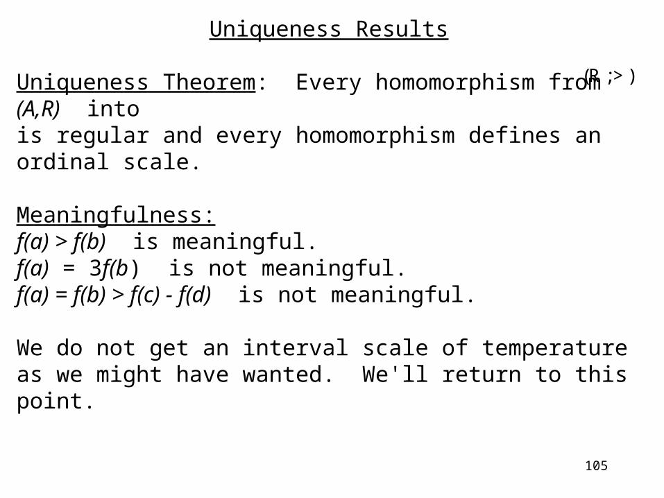
Uniqueness Results

Uniqueness Theorem: Every homomorphism from (A,R) into is regular and every homomorphism defines an ordinal scale.

Meaningfulness:f(a) > f(b) is meaningful.f(a) = 3f(b) is not meaningful.f(a) = f(b) > f(c) - f(d) is not meaningful.

We do not get an interval scale of temperature as we might have wanted. We'll return to this point.

(R ;>)

106

What Representations Lead to Ordinal Scales?

Let M be a positive integer. An M-tuple from corresponds to a strict weak order of rank first all i such that we never have ; having ranked , rank next all i such that for no , isThus, (3,9,3,2,8) has 2 ranked first, 5 ranked second, 1,3 tied for third, 4 last.

Suppose is a strict weak order on . Let on consist of all M-tuples whose corresponding ranking (strict weak order) is . E.g.: If . If = ,

(x1;x2; :::;xM )

R ¹M = f1;2;:::;M g:xj >xi i1, i2, ..., ip

j 6= i1, i2, ..., ip xj >xi :

¹M TM¼

R

(x1;x2; :::;xM )¼= f (1;2)g, T2

¼= f (x;y) : x > yg ©T2¼= f(x;y) : x = yg:

107

Theorem (Roberts 1984): Suppose S is an M-ary relation on and f is a homomorphism from (A,R) into which defines a regular ordinal scale. Suppose . Then S is of the form

where , ..., are all the strict weak orders of and is or

For example, if M = 2, then , , . So

R

(R ;S)jf (A)j ¸ M

S = (TM¼1)0[ (TM

¼2)0[ :::;

¼1, ¼2 ¹M (TM¼i)0

TM¼i

¼1 = f(1;2)g ¼2 = f(2;1)g

S = TM¼1[ TM

¼3is ¸ on R

S = TM¼1[ TM

¼2is 6= on R :

; :

¼3 = ;

108

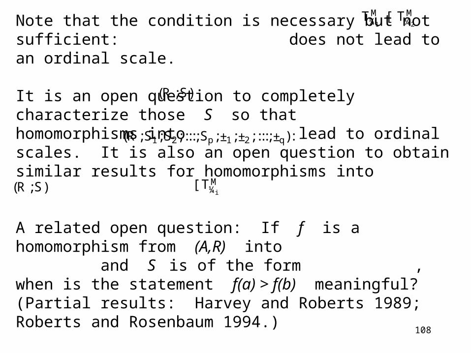
Note that the condition is necessary but not sufficient: does not lead to an ordinal scale.

It is an open question to completely characterize those S so that homomorphisms into lead to ordinal scales. It is also an open question to obtain similar results for homomorphisms into

A related open question: If f is a homomorphism from (A,R) into and S is of the form , when is the statement f(a) > f(b) meaningful? (Partial results: Harvey and Roberts 1989; Roberts and Rosenbaum 1994.)

TM¼1[ TM

¼2

(R ;S)

(R ;S1;S2; :::;Sp;±1;±2; :::;±q):

(R ;S) [ TM¼i

109

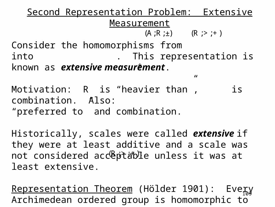
Second Representation Problem: Extensive Measurement

Consider the homomorphisms from into . This representation is known as extensive measurement.

Motivation: R is “heavier than”, is combination. Also: “preferred to” and combination.

Historically, scales were called extensive if they were at least additive and a scale was not considered acceptable unless it was at least extensive.

Representation Theorem (Hölder 1901): Every Archimedean ordered group is homomorphic to

(A;R;±) (R ;>;+)

±

(R ;>;+):

110

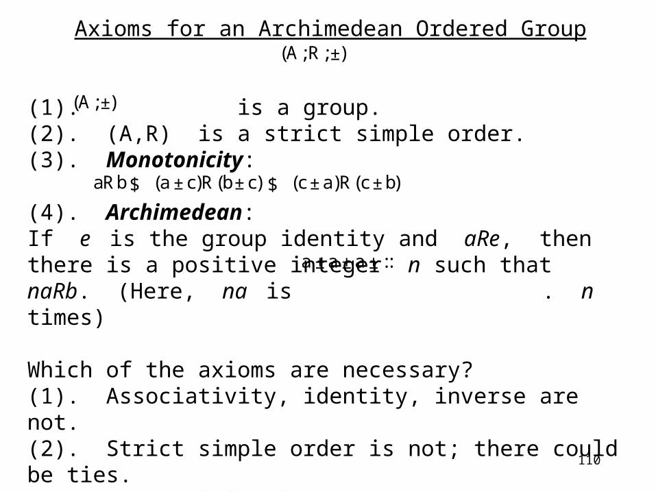
Axioms for an Archimedean Ordered Group

(1). is a group.(2). (A,R) is a strict simple order.(3). Monotonicity:

(4). Archimedean:If e is the group identity and aRe, then there is a positive integer n such that naRb. (Here, na is . n times)

Which of the axioms are necessary?(1). Associativity, identity, inverse are not.(2). Strict simple order is not; there could be ties.(3). Monotonicity is.(4). The Archimedean axiom as stated is not; it doesn't even make sense without e.

(A;R;±)

(A;±)

a±a±a±::

aRb$ (a±c)R(b±c) $ (c±a)R(c±b)

111

Definition: is an extensive structure if it satisfies the following conditions:

(1). Weak Associativity:

&

(2). (A,R) is a strict weak order.

(3). Monotonicity.

(4). Modified Archimedean Axiom: If aRb, then there is a positive integer n such that

(For the latter axiom, think of n(a-b) > (d-c).)

(A;R;±)

(na±c)R(nb±d):

~ ~ [(a±b) ±cRa±(b±c)][a±(b±c)R(a±b) ±c]

112

Theorem (Roberts and Luce 1968): is homomorphic to iff is an extensive structure.

Are the axioms reasonable? Descriptive?

For mass: OK

For preference:

Strict weak could be questioned. (Recall price-quality example.)

Weak associativity could be questioned if combination allows physical interaction:(a = flame, b = cloth, c = fire retardant)

(A;R;±)

(R ;>;+) (A;R;±)

113

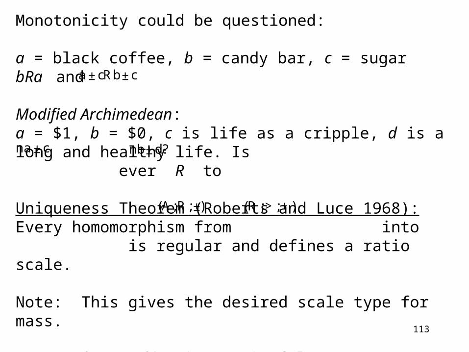
Monotonicity could be questioned:

a = black coffee, b = candy bar, c = sugarbRa and

Modified Archimedean:a = $1, b = $0, c is life as a cripple, d is a long and healthy life. Is ever R to

Uniqueness Theorem (Roberts and Luce 1968): Every homomorphism from into is regular and defines a ratio scale.

Note: This gives the desired scale type for mass.

Note: f(a) = 3f(b) is meaningful.

a±cRb±c

(A;R;±) (R ;>;+)

na±c nb±d?

114

Question: What representations into give rise to ratio scales?

Roberts (1984) showed that (A,R) into never gives rise to a ratio scale. Thus, requires at least two relations or at least one operation. Can we get a ratio scale without any operations in ?

(R ;S)

A

115

Third Representation Problem:Difference Measurement

Define on by

Let D be a quaternary relation on A. Consider the representation A homomorphism f satisfies

This representation is called algebraic difference measurement.

Motivation: Temperature measurement. D is comparison of differences in warmth. Related motivation: Utility with comparison of differences in value.

R

¢ (x;y;u;v) $ x ¡ y > u¡ v:

(A;D) ! (R ;¢ ):

D(a;b;c;d) $ f (a) ¡ f (b) > f (c) ¡ f (d):

116

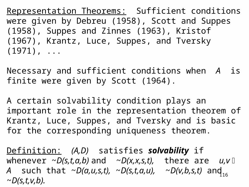
Representation Theorems: Sufficient conditions were given by Debreu (1958), Scott and Suppes (1958), Suppes and Zinnes (1963), Kristof (1967), Krantz, Luce, Suppes, and Tversky (1971), ...

Necessary and sufficient conditions when A is finite were given by Scott (1964).

A certain solvability condition plays an important role in the representation theorem of Krantz, Luce, Suppes, and Tversky and is basic for the corresponding uniqueness theorem.

Definition: (A,D) satisfies solvability if whenever ~D(s,t,a,b) and ~D(x,x,s,t), there are u,v A such that ~D(a,u,s,t), ~D(s,t,a,u), ~D(v,b,s,t) and ~D(s,t,v,b).

117

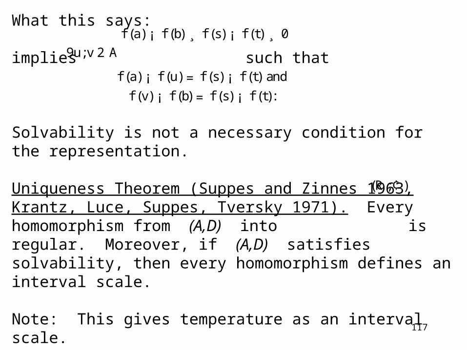
What this says:

implies such that

Solvability is not a necessary condition for the representation.

Uniqueness Theorem (Suppes and Zinnes 1963, Krantz, Luce, Suppes, Tversky 1971). Every homomorphism from (A,D) into is regular. Moreover, if (A,D) satisfies solvability, then every homomorphism defines an interval scale.

Note: This gives temperature as an interval scale.

f (a) ¡ f (b) ¸ f (s) ¡ f (t) ¸ 09u;v 2 A

f (a) ¡ f (u) = f (s) ¡ f (t) and

f (v) ¡ f (b) = f (s) ¡ f (t):

(R ;¢ )

118

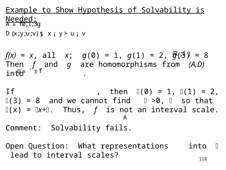
Example to Show Hypothesis of Solvability is Needed:

f(x) = x, all x; g(0) = 1, g(1) = 2, g(3) = 8Then f and g are homomorphisms from (A,D) into .

If , then (0) = 1, (1) = 2, (3) = 8 and we cannot find >0, so that (x) = x+. Thus, f is not an interval scale.

Comment: Solvability fails.

Open Question: What representations into lead to interval scales?

A = f0;1;3g

(R ;¢ )

g= ' ±f

D(x;y;u;v) $ x ¡ y > u¡ v

A

119

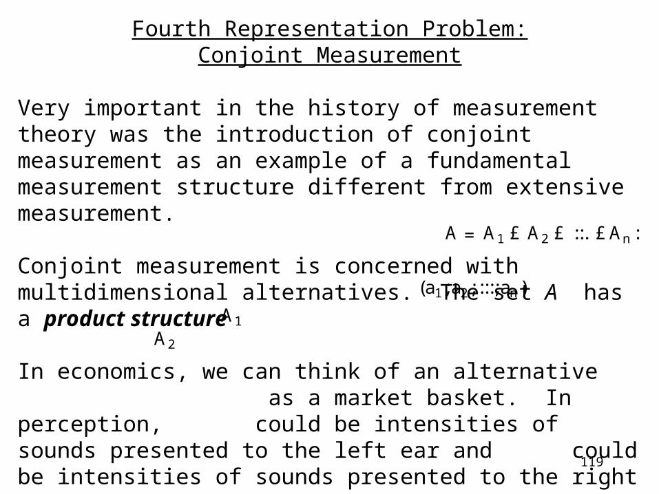
Fourth Representation Problem:Conjoint Measurement

Very important in the history of measurement theory was the introduction of conjoint measurement as an example of a fundamental measurement structure different from extensive measurement.

Conjoint measurement is concerned with multidimensional alternatives. The set A has a product structure

In economics, we can think of an alternative as a market basket. In perception, could be intensities of sounds presented to the left ear and could be intensities of sounds presented to the right ear.

A =A1 £ A2 £ ::. £An :

(a1;a2; :::;an)

A1

A2

120

In testing, set could be a set of subjects and set a set of test items. In studying response strength, we could take a combination of drive and incentive. And so on.

We have a binary relation on A interpreted as “preferred to”, “sounds louder”, “performs better”, etc. We seek functions so that

Sufficient conditions for the representation were given by Debreu [1960] and Luce & Tukey [1964]; necessary and sufficient conditions by Scott [1964] in case each is finite.

A1 A2

f i : A i ! R

f 1(a1) + f 2(a2) + :::+ f n(an) >

f 1(b1) + f 2(b2) + :::+ f n(bn):

A i

(a1;a2; :::;an)R(b1;b2; :::;bn) $

121

Semiorders

Suppose R is preference.

Recall that indifference corresponds to the relation:

aIb ~aRb & ~bRa

Suppose f is an ordinal utility function:

aRb f(a) > f(b)

Then

aIb f(a) = f(b)

This implies that indifference is transitive.

$

$

$

122

Arguments against transitivity of indifference (or more generally of “tying” in a measurement context) go back to Armstrong in the 1930's, Wiener in the 1920's, even Poincaré (in the 19th century).

One argument against transitivity of indifference: The Coffee-Sugar example (Luce 1956).

Let 0* = cup of coffee with no sugar, 5* = cup of coffee with 5 spoons of sugar.

We have a preference between 0* and 5* -- we are not indifferent.

0* 5*

123

Arguments against transitivity of indifference (or more generally of “tying” in a measurement context) go back to Armstrong in the 1930's, Wiener in the 1920's, even Poincaré (in the 19th century).

One argument against transitivity of indifference: The Coffee-Sugar example (Luce 1956).

Let 0* = cup of coffee with no sugar, 5* = cup of coffee with 5 spoons of sugar.

We have a preference between 0* and 5* -- we are not indifferent.

Add sugar one grain at a time. We are indifferent between the first and the last.

0* 5*

124

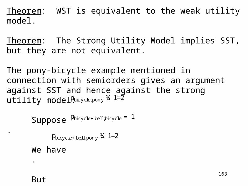
Second argument against transitivity of indifference: Pony-bicycle Example (Armstrong 1939):

pony I bicycle

pony I bicycle+bell

not bicycle I bicycle+bell

The semiorder model we shall discuss is intended to account for the first kind of problem, but not the second.

125

The Idea: Find a function f so that

aRb f(a) is “sufficiently larger” than f(b)

Let > 0 be a threshold or just noticeable difference. Find a function f on A so that

aRb f(a) > f(b) +

Define > on by

We are seeking a homomorphism from (A,R) into

R

(R ;>±):

$

$

x >±y $ x > y+±:

126

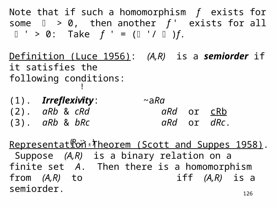
Note that if such a homomorphism f exists for some > 0, then another f ' exists for all ' > 0: Take f ' = ( '/ )f.

Definition (Luce 1956): (A,R) is a semiorder if it satisfies the following conditions:

(1). Irreflexivity: ~aRa(2). aRb & cRd aRd or cRb(3). aRb & bRc aRd or dRc.

Representation Theorem (Scott and Suppes 1958). Suppose (A,R) is a binary relation on a finite set A. Then there is a homomorphism from (A,R) to iff (A,R) is a semiorder.(R ;>±)

!

!

127

Necessity of the conditions:

(1). trivial

(3).

(2). If f(a) f(c):

If f(a) f(c):

f(c) f(b) f(a)

f(d) f(c) f(a)

f(b) f(a) f(c)

( )

( )

( )

( )

128

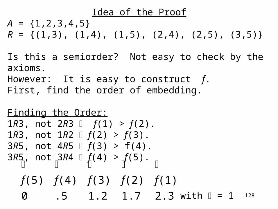
Idea of the ProofA = {1,2,3,4,5}R = {(1,3), (1,4), (1,5), (2,4), (2,5), (3,5)}

Is this a semiorder? Not easy to check by the axioms.However: It is easy to construct f.First, find the order of embedding.

Finding the Order:1R3, not 2R3 f(1) > f(2).1R3, not 1R2 f(2) > f(3).3R5, not 4R5 f(3) > f(4).3R5, not 3R4 f(4) > f(5).

f(5) f(4) f(3) f(2) f(1)

0 .5 1.2 1.7 2.3 with = 1

129

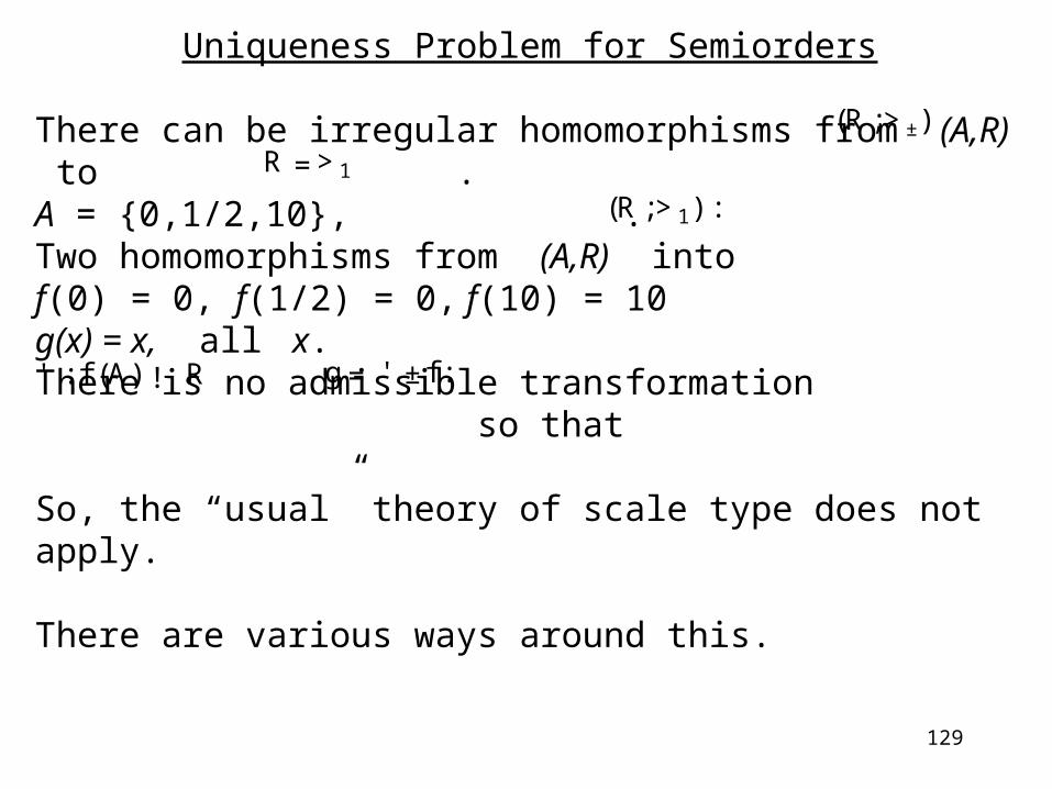
Uniqueness Problem for Semiorders

There can be irregular homomorphisms from (A,R) to . A = {0,1/2,10}, .Two homomorphisms from (A,R) intof(0) = 0, f(1/2) = 0, f(10) = 10g(x) = x, all x.There is no admissible transformation so that

So, the “usual” theory of scale type does not apply.

There are various ways around this.

(R ;>±)R =>1

(R ;>1) :

' : f (A) ! R g= ' ±f :

130

The Method of Perfect Substitutes

Define an equivalence relation E on A by:

In this case, a and b are perfect substitutes for each other with respect to the relation R. Define on the collection of equivalence classes by:

If (A,R) is a semiorder, is well-defined and is again a semiorder. Moreover, every homomorphism is now 1-1 and regular.

R¤

A¤

R¤

a¤R¤b¤ $ aRb:

aEb$ (8c)(aRc$ bRc & cRa$ cRb):

131

A similar trick of canceling out the perfect substitutes relation E always leads to regular representations for equivalence classes.

We can now ask: What is the scale type of a homomorphism from into None of the common scale types applies and no succinct characterization of admissible transformations is known.

A Uniqueness ResultSuppose

Define W on A by:

Then (A,W) is a strict weak order.

(A¤;R¤) (R ;>±)?

aRb$ f (a) > f (b) +±:

aWb$ f (a) > f (b).

132

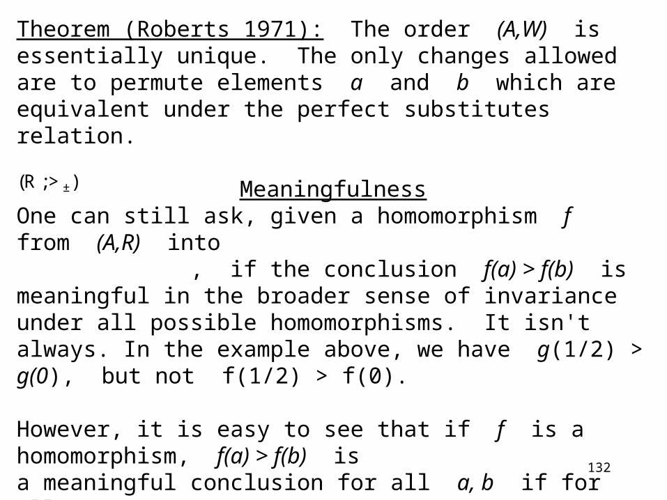
Theorem (Roberts 1971): The order (A,W) is essentially unique. The only changes allowed are to permute elements a and b which are equivalent under the perfect substitutes relation.

MeaningfulnessOne can still ask, given a homomorphism f from (A,R) into , if the conclusion f(a) > f(b) is meaningful in the broader sense of invariance under all possible homomorphisms. It isn't always. In the example above, we have g(1/2) > g(0), but not f(1/2) > f(0).

However, it is easy to see that if f is a homomorphism, f(a) > f(b) is a meaningful conclusion for all a, b if for all x y, ~xEy.

(R ;>±)

133

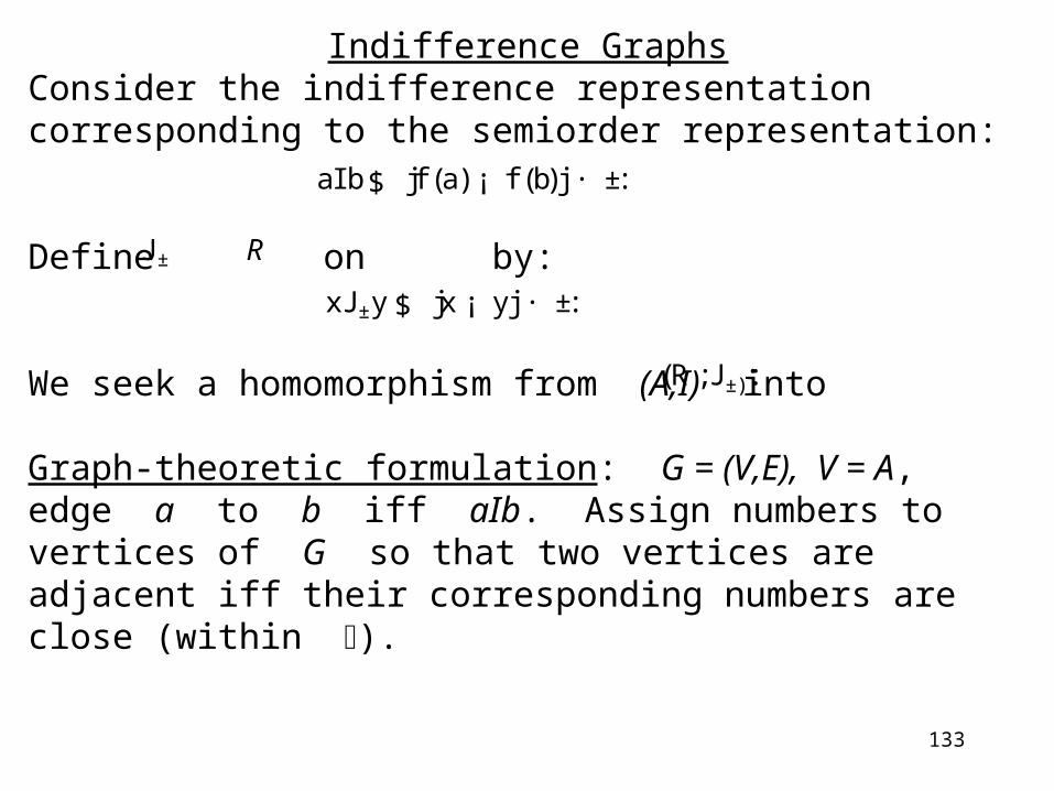
Indifference GraphsConsider the indifference representation corresponding to the semiorder representation:

Define on by:

We seek a homomorphism from (A,I) into

Graph-theoretic formulation: G = (V,E), V = A, edge a to b iff aIb. Assign numbers to vertices of G so that two vertices are adjacent iff their corresponding numbers are close (within ).

J ± R

(R ;J ±):

aI b$ jf (a) ¡ f (b)j · ±:

xJ ±y $ jx ¡ yj · ±:

134

1.1

0 .7 1.6 2.5

= 1

Here is an example of such a representation on a graph:

Definition: We say that (A,I) is an indifference graph if there is a homomorphism into (R ;J ±):

135

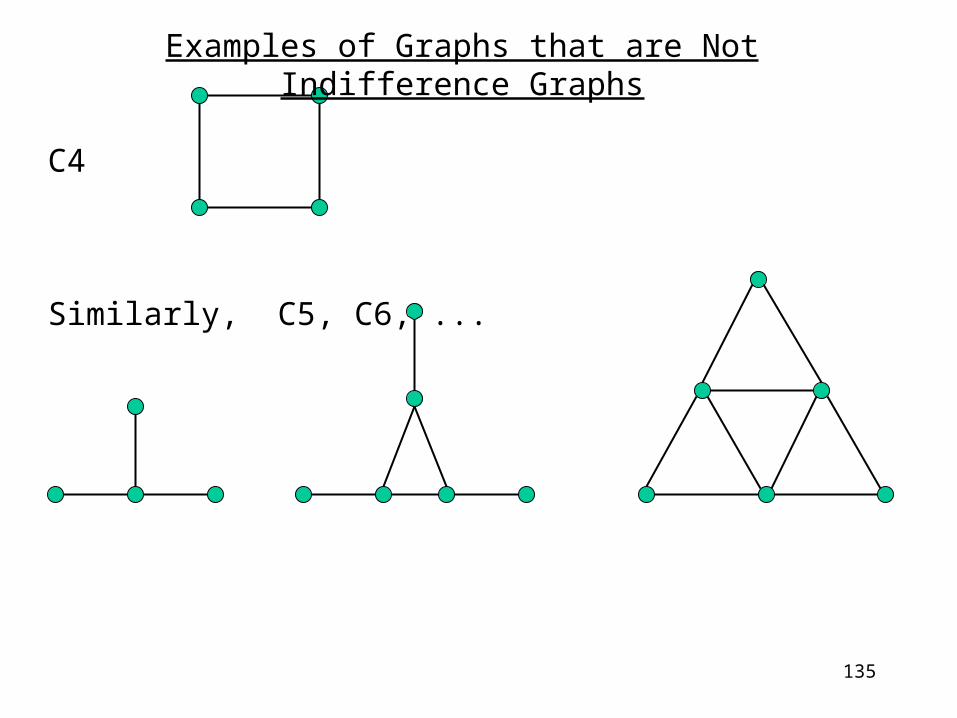
Examples of Graphs that are Not Indifference Graphs

C4

Similarly, C5, C6, ...

136

Representation Theorem (Roberts 1969). G = (A,I) is an indifference graph iff it has none of the above graphs as an induced subgraph.

Uniqueness:Irregularity can again be a problem. Now, the perfect substitutes relation is equivalent to:

(Assuming that aIa for all a, we have aEb iff a and b have the same closed neighborhoods.)

Define on by . Then all homomorphisms from into are regular, but the class of admissible transformations is not known.

I ¤ A¤

(A¤; I ¤) (R ;J ±)

aEb$ (8c)(aI c$ bI c)

a¤I ¤b¤ $ aI b

137

Again, is essentially unique, as in the case of semiorders.

Meaningfulness

f(a) > f(b) is never meaningful for indifference graphs since -f is again a homomorphism. However, some ordinal conclusions are meaningful.

Say y is between x and z if x<y<z or z<y<x. Betweenness is a significant observation in psychophysical and perceptual experiments and in judgments of worth or value. When is the conclusion that f(b) is between f(a) and f(c) meaningful?

aWb$ f (a) > f (b)

138

Theorem (Roberts 1984). Suppose A is finite and f is a homomorphism from (A,I) into . Then the conclusion that f(b) is between f(a) and f(c) is meaningful for all a,b,c in A iff (A,I) is connected as a graph and for all x y in A, ~xEy.

It is an open question to generalize this result beyond indifference graphs and determine for what representations the conclusion that f(b) is between f(a) and f(c) is meaningful for all a,b,c.

(R ;J ±)

139

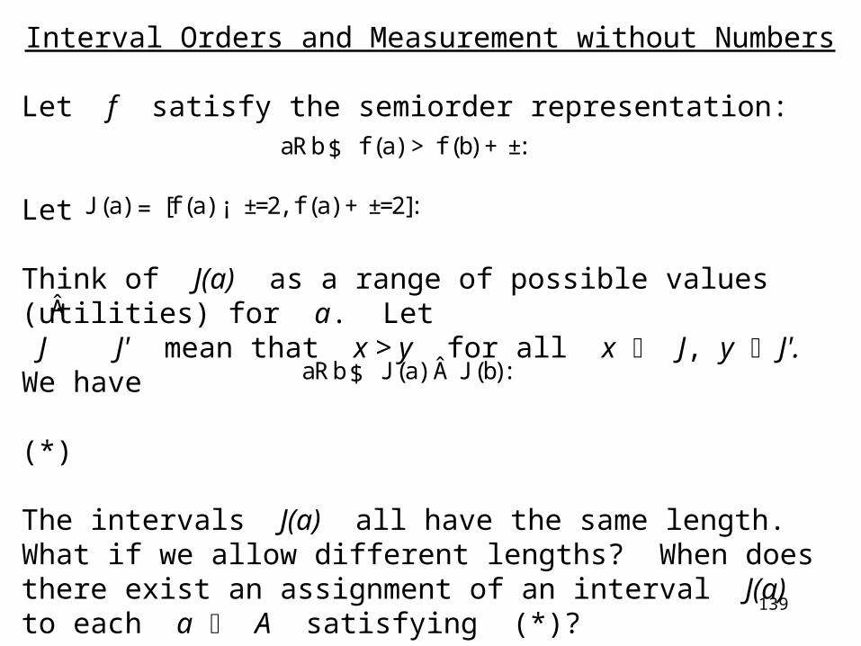
Interval Orders and Measurement without Numbers

Let f satisfy the semiorder representation:

Let

Think of J(a) as a range of possible values (utilities) for a. Let J J' mean that x > y for all x J, y J'. We have

(*)

The intervals J(a) all have the same length. What if we allow different lengths? When does there exist an assignment of an interval J(a) to each a A satisfying (*)?

J (a) = [f (a) ¡ ±=2, f (a) +±=2]:

aRb$ f (a) > f (b) +±:

aRb$ J (a) Â J (b):

Â

140

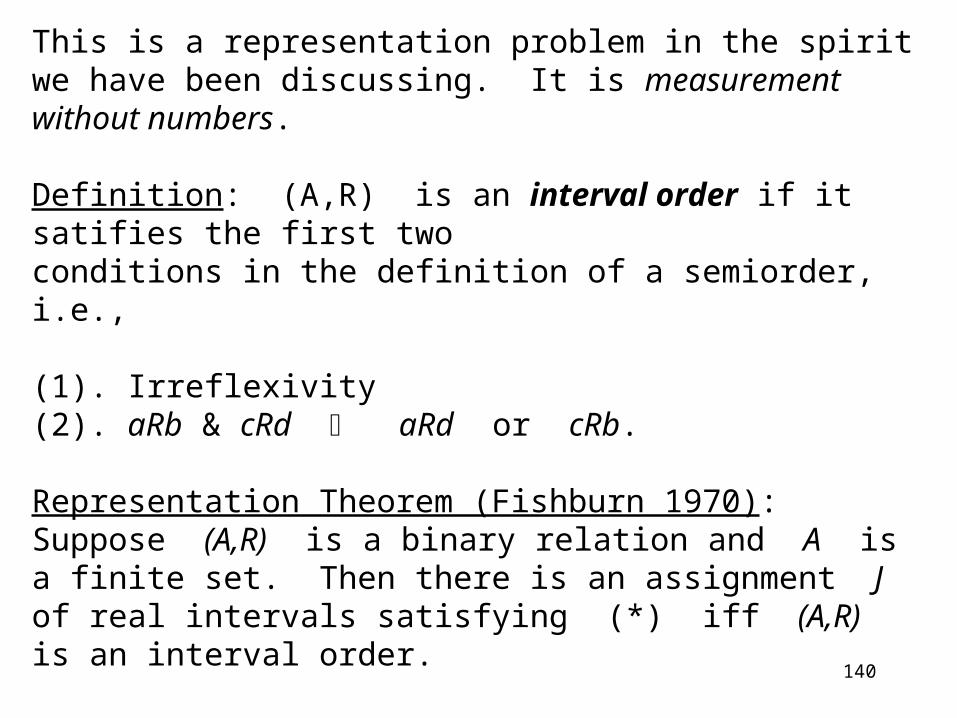
This is a representation problem in the spirit we have been discussing. It is measurement without numbers.

Definition: (A,R) is an interval order if it satifies the first two conditions in the definition of a semiorder, i.e.,

(1). Irreflexivity(2). aRb & cRd aRd or cRb.

Representation Theorem (Fishburn 1970): Suppose (A,R) is a binary relation and A is a finite set. Then there is an assignment J of real intervals satisfying (*) iff (A,R) is an interval order.

141

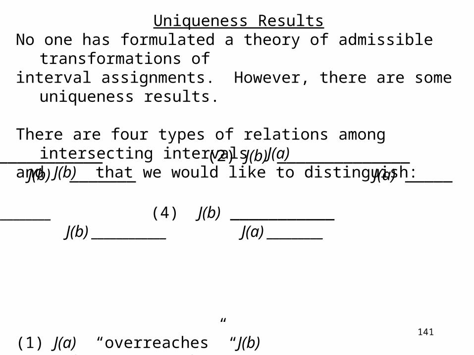
Uniqueness ResultsNo one has formulated a theory of admissible transformations ofinterval assignments. However, there are some uniqueness results.

There are four types of relations among intersecting intervals J(a)and J(b) that we would like to distinguish:

(1) J(a) “overreaches” J(b)(2) J(b) “overreaches” J(a)(3) J(a) “weakly precedes” J(b)(4) J(b) “weakly precedes” J(a).

(1) J(a) ____________ (2) J(b) ______________ J(b) _______ J(a) _____

(3) J(a) ___________ (4) J(b) ___________ J(b) ____________ J(a) _________

142

One interesting question is to try to determine when the conclusion that J(a) overreaches J(b) is meaningful. These questions arise in economics when the intervals are ranges of possible values of a commodity. They also arise in archaeological seriation when these are intervals of time during which a particular type of artifact was in use. In the latter context, Skrien (1980,1984) developed an O(n3) algorithm for determining if these conclusions are meaningful.

143

Interval Graphs

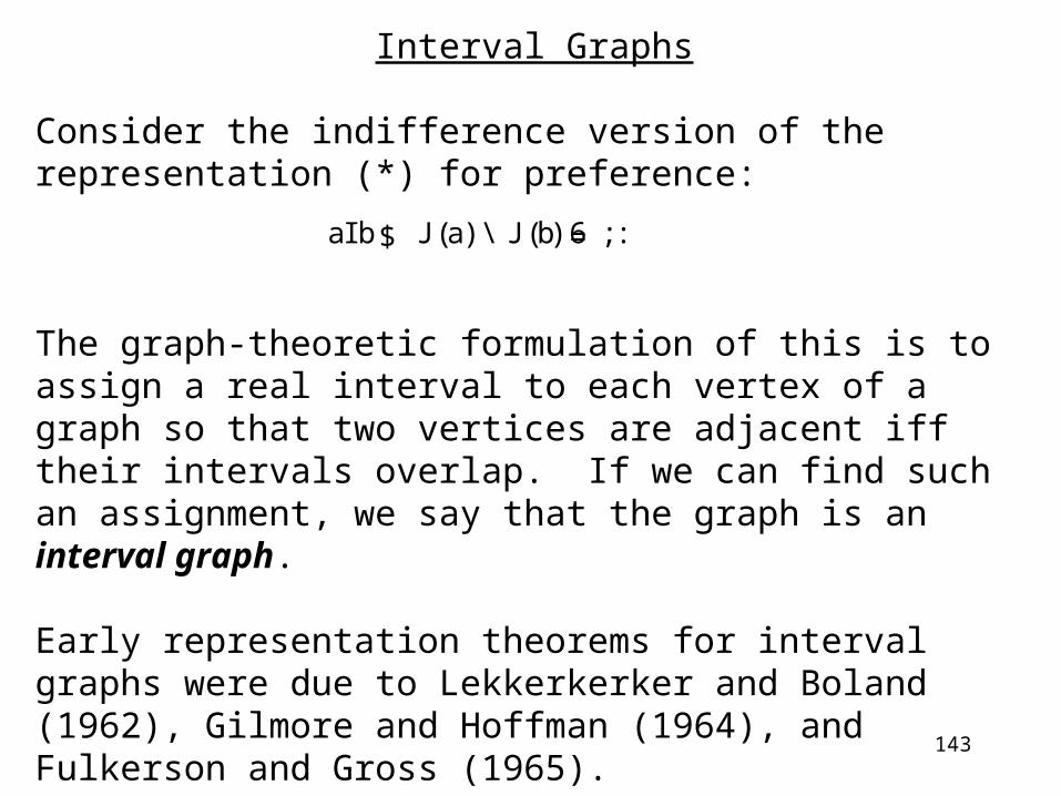
Consider the indifference version of the representation (*) for preference:

The graph-theoretic formulation of this is to assign a real interval to each vertex of a graph so that two vertices are adjacent iff their intervals overlap. If we can find such an assignment, we say that the graph is an interval graph.

Early representation theorems for interval graphs were due to Lekkerkerker and Boland (1962), Gilmore and Hoffman (1964), and Fulkerson and Gross (1965).

aI b$ J (a) \ J (b) 6= ; :

144

Interval graphs have numerous applications, in archaeology, developmental psychology, molecular biology, scheduling, traffic phasing, ecology, computer science, etc.

Uniqueness Questions

Uniqueness questions similar to those about interval orders arise. For example, when are conclusions about overreaching and weak precedence meaningful? We have an additional question here: How unique are conclusions J(a) J(b)? These are never meaningful, since we can always “reverse” all intervals. However, induces a transitive orientation on the complement of the graph in question, and the uniqueness of transitive orientations has been widely studied.

ÂÂ

Â

145

Higher Dimensional Intersection Graphs

Consider again

What if the J(a)'s are other objects, such as boxes, cubes, spheres, arcs on a circle, etc.? One can ask representation and uniqueness questions about these situations. For the most part, these questions are unsolved. For instance, we still don't know a representation theorem if the J(a) are rectangles in the plane (with sides parallel to the coordinate axes), or squares.

aI b$ J (a) \ J (b) 6= ; :

146

Partial Orders

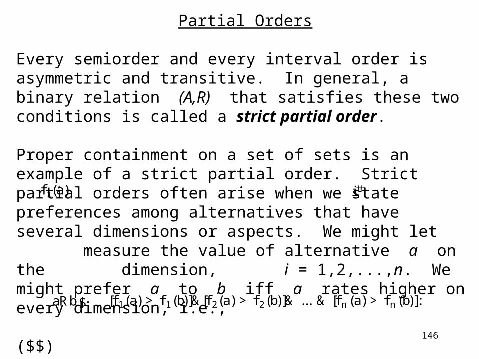
Every semiorder and every interval order is asymmetric and transitive. In general, a binary relation (A,R) that satisfies these two conditions is called a strict partial order.

Proper containment on a set of sets is an example of a strict partial order. Strict partial orders often arise when we state preferences among alternatives that have several dimensions or aspects. We might let measure the value of alternative a on the dimension, i = 1,2,...,n. We might prefer a to b iff a rates higher on every dimension, i.e.,

($$)

ithf i (a)

aRb$ [f 1(a) > f 1(b)]&[f 2(a) > f 2(b)]& ... & [f n(a) > f n(b)]:

147

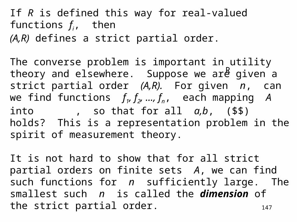
If R is defined this way for real-valued functions fi, then (A,R) defines a strict partial order.

The converse problem is important in utility theory and elsewhere. Suppose we are given a strict partial order (A,R). For given n, can we find functions f1, f2, ..., fn, each mapping A into , so that for all a,b, ($$) holds? This is a representation problem in the spirit of measurement theory.

It is not hard to show that for all strict partial orders on finite sets A, we can find such functions for n sufficiently large. The smallest such n is called the dimension of the strict partial order.

R

148

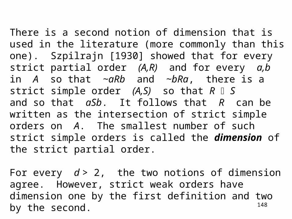
There is a second notion of dimension that is used in the literature (more commonly than this one). Szpilrajn [1930] showed that for every strict partial order (A,R) and for every a,b in A so that ~aRb and ~bRa, there is a strict simple order (A,S) so that R Sand so that aSb. It follows that R can be written as the intersection of strict simple orders on A. The smallest number of such strict simple orders is called the dimension of the strict partial order.

For every d > 2, the two notions of dimension agree. However, strict weak orders have dimension one by the first definition and two by the second.

149

Example:

This is a strict partial order. It is the intersection of two strict simple orders: the order ranking a over b over c over d and the order ranking a over d over b over c.

We can also find two functions f1 and f2 satisfying ($$):

f1(a) = 4, f1(b) = 3, f1(c) = 2, f1(d) = 1,

f2(a) = 4, f2(d) = 3, f2(b) = 2, f2(c) = 1.

A = fa;b;c;dg, R = f (a;b), (b;c), (a;c), (a;d)g

150

Partial Orders vs. Strict Partial Orders

We shall use the term partial order for the binary relations related to strict partial orders in the same way that weak orders are related to strict weak orders. Thus, proper containment on a set of sets defines a strict partial order, while containment defines a partial order.

Formally, we say that (A,R) is a partial order if it is reflexive, transitive, and antisymmetric.

151

Subjective ProbabilityWhen we say that one event seems more probable than another, we are making subjective comparisons of probabilities. One can ask when such comparisons are consistent with a probability measure.

Formalization of this question: We say that is an algebra of events if elements of are subsets of X and is closed under union and complementation. We say that a function p on an algebra of events is a finitely additive probability measure if p is a real-valued function from so that

(1). p(A) 0(2). p(X) = 1(3).

(X ;E)

E E

E

p(A [ B) = p(A) +p(B) if A \ B = ; :

152

Suppose is an algebra of events and is a binary relation on , with A B interpreted to mean that A is (subjectively) judged more probable than B. Does there exist a finitely additive probability measure p on which “preserves” , i.e., so that for all A, ,

(%)

Such a measure p is called a subjective probability measure. We can ask for representation and uniqueness theorems in the spirit of representational measurement theory.

(X ;E)

E

(X ;E)B 2 E

A Â B $ p(A) > p(B):

Â

Â

Â

153

The study of the comparative probability relation goes back at least to Bernstein (1917). The following necessary conditions for the representation (%) go back to Bruno de Finetti (1937).

de Finetti Axioms

(1). is a strict weak order.

(2). and , where A B means that ~B A.

(3). Monotonicity: If , then

(E;Â)

X Â ; A º ;

A \ B = A \ C = ;

B Â C $ A [ B Â A [ C:

Â

Â

Â

154

The axioms are clearly necessary. That they are not sufficient was shown by Savage in 1954 for infinite and by Kraft, Pratt, and Seidenberg in 1959 for finite.

Representation Theorems

Scott (1964) gave necessary and sufficient conditions in the case where is finite and Suppes and Zanotti (1976) gave necessary and sufficient conditions for arbitrary .

Perhaps historically one of the most interesting non-necessary axioms is the following:

E

E

E

E

155

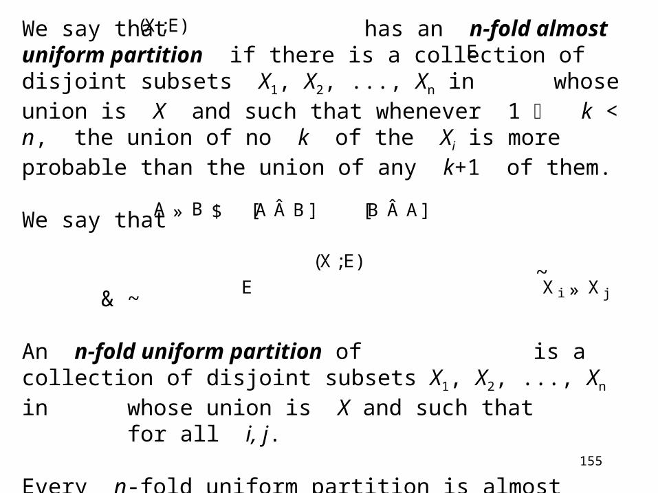
We say that has an n-fold almost uniform partition if there is a collection of disjoint subsets X1, X2, ..., Xn in whose union is X and such that whenever 1 k < n, the union of no k of the Xi is more probable than the union of any k+1 of them.

We say that

~ & ~

An n-fold uniform partition of is a collection of disjoint subsets X1, X2, ..., Xn in whose union is X and such that for all i, j.

Every n-fold uniform partition is almost uniform.

(X ;E)E

(X ;E)E X i » X j

[A Â B] [B Â A]A » B $

156

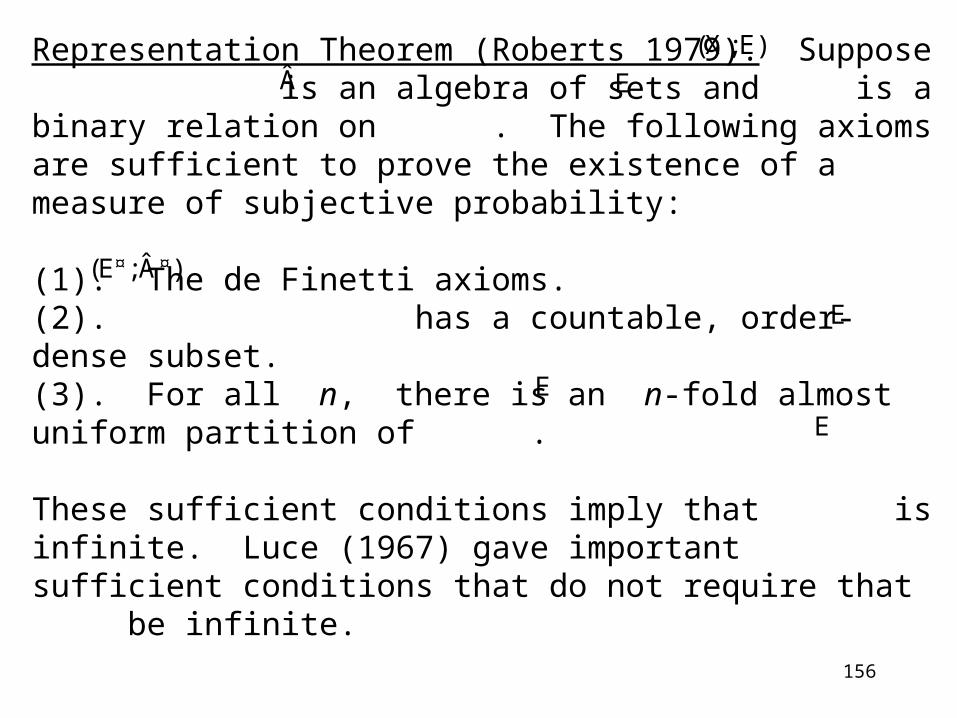
Representation Theorem (Roberts 1979). Suppose is an algebra of sets and is a binary relation on . The following axioms are sufficient to prove the existence of a measure of subjective probability:

(1). The de Finetti axioms.(2). has a countable, order-dense subset.(3). For all n, there is an n-fold almost uniform partition of .

These sufficient conditions imply that is infinite. Luce (1967) gave important sufficient conditions that do not require that be infinite.

(X ;E)E

(E¤;¤)

E

E

E

Â

157

Uniqueness Results

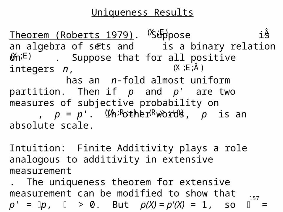
Theorem (Roberts 1979). Suppose is an algebra of sets and is a binary relation on . Suppose that for all positive integers n, has an n-fold almost uniform partition. Then if p and p' are two measures of subjective probability on , p = p'. In other words, p is an absolute scale.

Intuition: Finite Additivity plays a role analogous to additivity in extensive measurement . The uniqueness theorem for extensive measurement can be modified to show that p' = p, > 0. But p(X) = p'(X) = 1, so = 1.

(X ;E)

E(X ;E)

(X ;E;Â)

((A;R;±) ! (R ;>;+))

Â

158

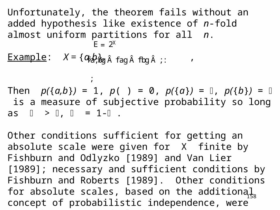
Unfortunately, the theorem fails without an added hypothesis like existence of n-fold almost uniform partitions for all n.

Example: X = {a,b}, ,

Then p({a,b}) = 1, p( ) = 0, p({a}) = , p({b}) = is a measure of subjective probability so long as > , = 1- .

Other conditions sufficient for getting an absolute scale were given for X finite by Fishburn and Odlyzko [1989] and Van Lier [1989]; necessary and sufficient conditions by Fishburn and Roberts [1989]. Other conditions for absolute scales, based on the additional concept of probabilistic independence, were given by Suppes and Alechina [1994].

E = 2X

f a;bg fag fbg ; :

;

159

Probabilistic Consistency

If judgments are made repeatedly, individuals are often inconsistent. For example, a subject might prefer a to b once, b to a later; or say that a is warmer than b once, b is warmer than a later. Let pab represent the proportion of times that a is preferred to b, or a is judged warmer than b, etc.

Then p is a function from A into [0,1]. Call (A,p) a forced choice pair comparison system (fcpcs) if for all a,b in A, pab + pba = 1.

We try to capture the idea that the individual, while being inconsistent, is being consistent in a probabilistic sense.

160

Definition: A fcpcs satisfies the weak utility model if there is so that for all a,b in A,

Representation and Uniqueness Theorems: Define W on A by

Then (A,p) satisfies the weak utility model iff (A,W) is homomorphic to . Moreover, if f is a function satisfying the weak utility model, then f defines a (regular) ordinal scale.

f : A ! R

(R ;>)

pab>pba $ f (a) > f (b):

aWb$ pab>pba:

161

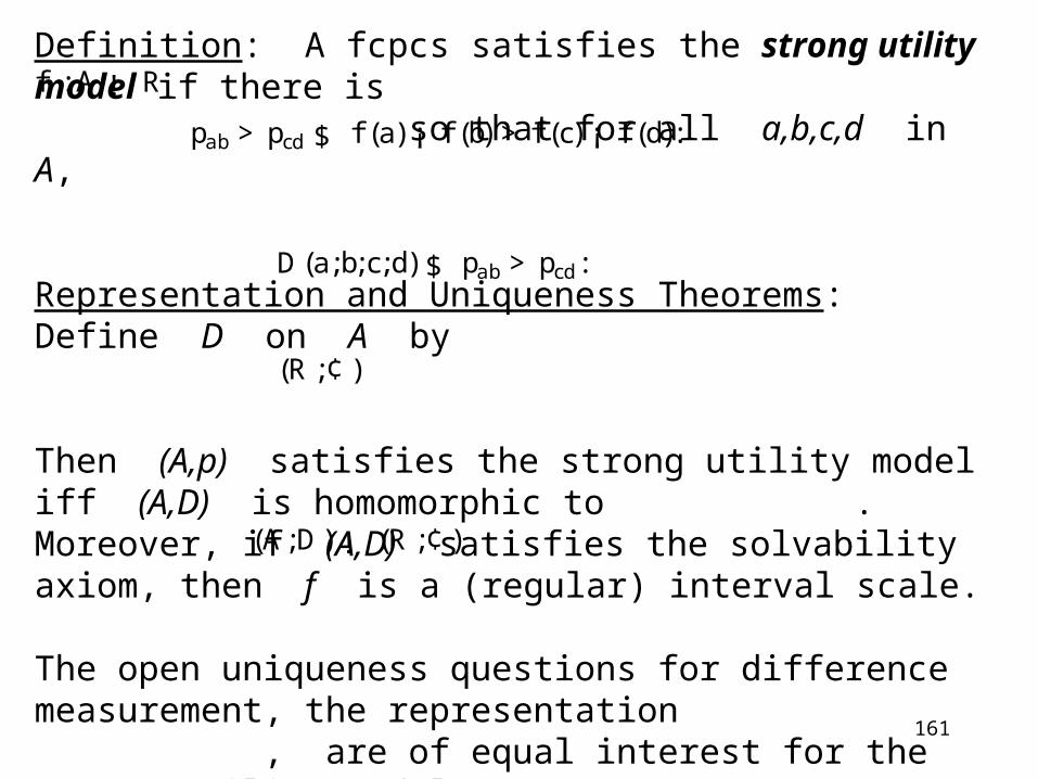
Definition: A fcpcs satisfies the strong utility model if there is so that for all a,b,c,d in A,

Representation and Uniqueness Theorems: Define D on A by

Then (A,p) satisfies the strong utility model iff (A,D) is homomorphic to . Moreover, if (A,D) satisfies the solvability axiom, then f is a (regular) interval scale.

The open uniqueness questions for difference measurement, the representation , are of equal interest for the strong utility model.

f : A ! R

(R ;¢ )

pab>pcd $ f (a) ¡ f (b) > f (c) ¡ f (d):

D(a;b;c;d) $ pab>pcd:

(A;D) ! (R ;¢ )

162

Stochastic Transitivity Conditions

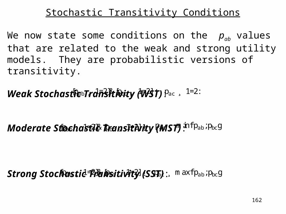
We now state some conditions on the pab values that are related to the weak and strong utility models. They are probabilistic versions of transitivity.

Weak Stochastic Transitivity (WST):

Moderate Stochastic Transitivity (MST):

Strong Stochastic Transitivity (SST):

pac ¸ minfpab;pbcg

pac ¸ maxfpab;pbcg

[pab ¸ 1=2]&[pbc ¸ 1=2] ! pac ¸ 1=2:

[pab ¸ 1=2]&[pbc ¸ 1=2] !

[pab ¸ 1=2]&[pbc ¸ 1=2] !

163

Theorem: WST is equivalent to the weak utility model.

Theorem: The Strong Utility Model implies SST, but they are not equivalent.

The pony-bicycle example mentioned in connection with semiorders gives an argument against SST and hence against the strong utility model:

Suppose .

We have .

But .

pbicycle;pony ¼1=2

pbicycle+bell;bicycle =1

pbicycle+bell;pony ¼1=2

164

Homogeneous Families of Semiorders

In experiments with loudness judgments, we often take a to be louder than b (or beyond threshold) if it is judged to be louder a sufficiently high percentage of the time, like 3/4. Given a number [1/2,1), we can define a binary relation R on A by:

Luce [1958,1959] showed that under certain conditions, each (A,R) is a semiorder. For instance, SST implies this conclusion. Thus, under SST, is a family of semiorders.

F = f (A;R¸ ) : ¸ 2 [1=2;1)g

aR¸b$ pab> ¸:

165

We have noted that for a semiorder (A,R), the order in which the elements are mapped into the reals under a homomorphism into is essentially unique. This order is sometimes called the compatible weak order.

We shall call a family of semiorders on the same underlying set homogeneous if there is one weak order compatible with all of the semiorders in the family. It turns out that under SST, is a homogeneous family of semiorders. This is another condition of probabilistic consistency.

The converse is also true under one additional assumption.

(R ;>±)

F

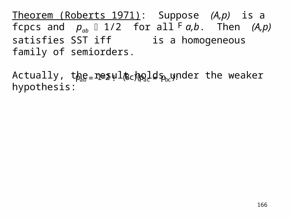
166

Theorem (Roberts 1971): Suppose (A,p) is a fcpcs and pab 1/2 for all a,b. Then (A,p) satisfies SST iff is a homogeneous family of semiorders.

Actually, the result holds under the weaker hypothesis:

F

pab=1=2! (8c)(pac =pbc):

167

x y

20

a1 2

Meaningfulness of Conclusions from Combinatorial Optimization(Roberts 1990)

What conclusions about optimal solutions or algorithms are meaningful?

Shortest Path Problem

What is the shortest path from x to y?

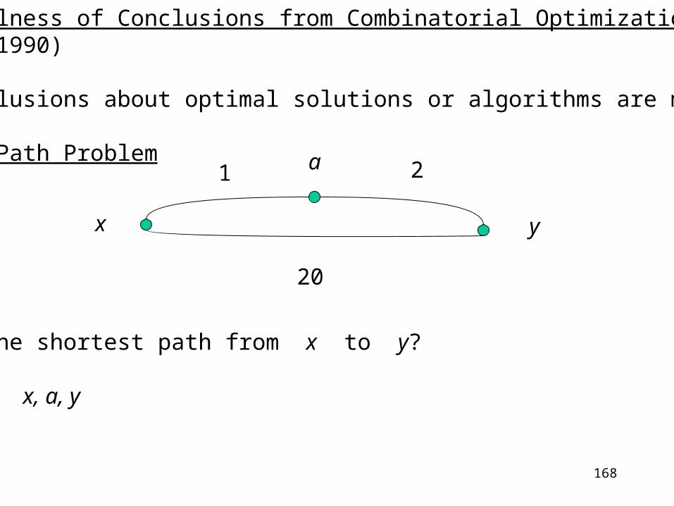
168

x y

20

a1 2

Meaningfulness of Conclusions from Combinatorial Optimization(Roberts 1990)

What conclusions about optimal solutions or algorithms are meaningful?

Shortest Path Problem

What is the shortest path from x to y?

Solution: x, a, y

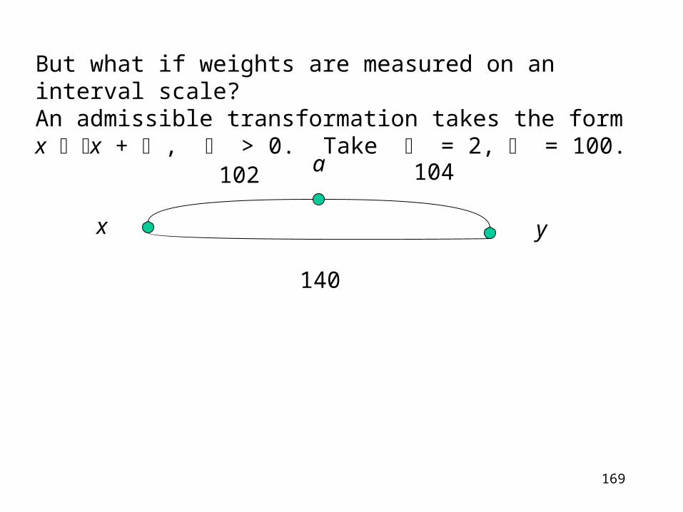
169

x y

140

a102 104

But what if weights are measured on an interval scale?An admissible transformation takes the form x x + , > 0. Take = 2, = 100.

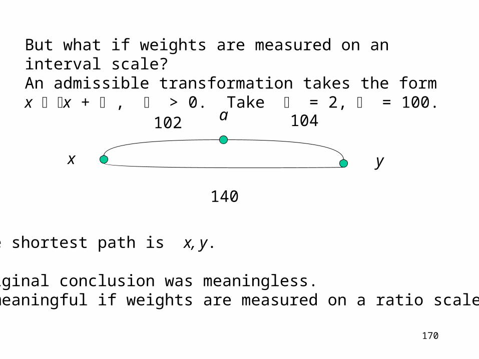
170

x y

140

a102 104

But what if weights are measured on an interval scale?An admissible transformation takes the form x x + , > 0. Take = 2, = 100.

Now the shortest path is x, y.

The original conclusion was meaningless.It is meaningful if weights are measured on a ratio scale.

171

Linear ProgrammingThe shortest path problem can be formulated as a linear programming problem. The above discussion illustrates the following point: The conclusion that z is an optimal solution in a LPP can be meaningless if the cost parameters are measured on an interval scale.

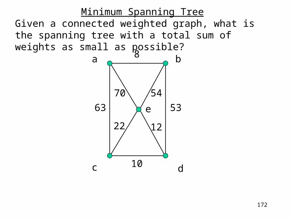
172

a b

c d

e

8

63 53

10

70

22

54

12

Minimum Spanning TreeGiven a connected weighted graph, what is the spanning tree with a total sum of weights as small as possible?

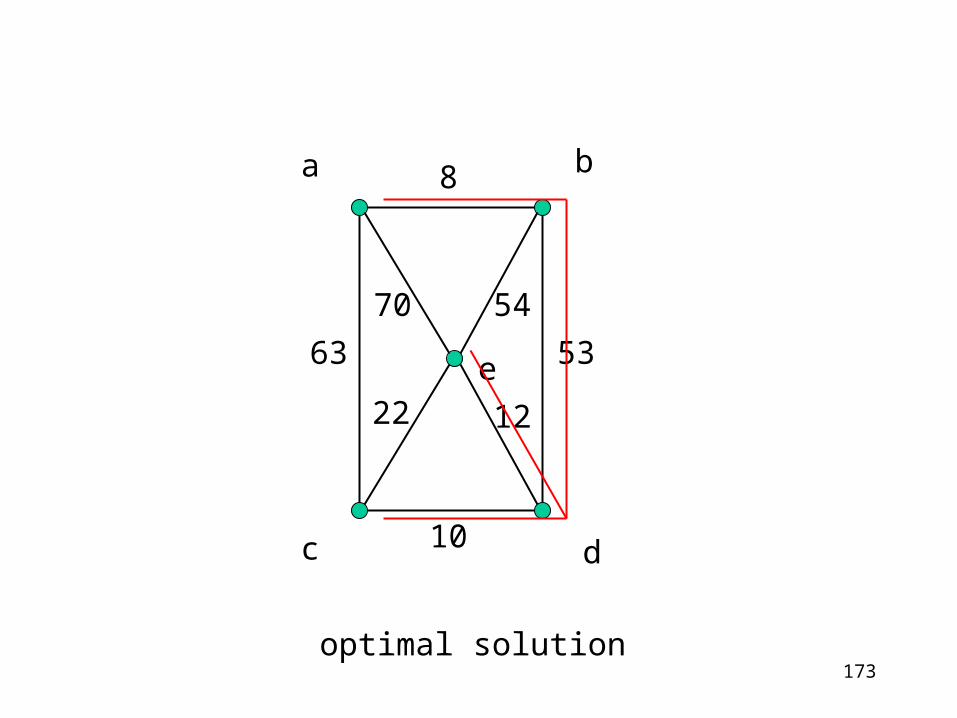
173

a b

c d

e

8

63 53

10

70

22

54

12

optimal solution

174

What if we change weights, say by an admissible transformation for interval scales?Say we take x x + with = 2, = 100. We get the following weighted graph.

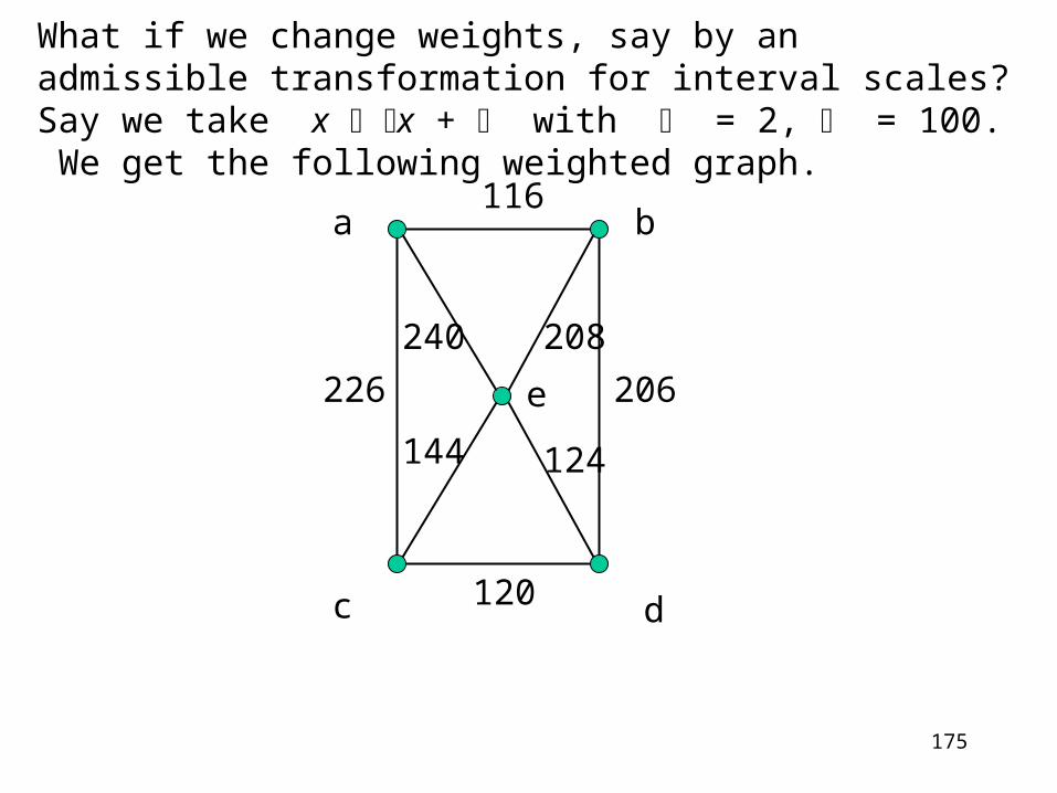
175

a b

c d

e

116

226 206

120

240

144

208

124

What if we change weights, say by an admissible transformation for interval scales?Say we take x x + with = 2, = 100. We get the following weighted graph.

176

a b

c d

e

116

226 206

120

240

144

208

124

optimal solution

177

The optimal solution is the same. Is this an accident?

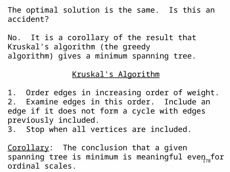
178

The optimal solution is the same. Is this an accident?

No. It is a corollary of the result that Kruskal's algorithm (the greedy algorithm) gives a minimum spanning tree.

Kruskal's Algorithm

1. Order edges in increasing order of weight.2. Examine edges in this order. Include an edge if it does not form a cycle with edges previously included.3. Stop when all vertices are included.

Corollary: The conclusion that a given spanning tree is minimum is meaningful even for ordinal scales.

179

Note that analysis of meaningfulness is something like sensitivity analysis. However, the perturbations studied do not have to be small. We are investigating the sensitivity (or invariance) of conclusions under certain kinds of changes.

180

Frequency Assignment and T-ColoringThe following problem arises from questions of channel assignment.

Let G = (V,E) be a graph and T be a set of nonnegative integers. Find an assignment f of a positive integer f(x) to each vertex x in G so that

Such an f is called a T-coloring of G.In the application:V = set of transmitters;E means conflict;f(x) is channel assigned to transmitter x;T is a set of disallowed separations between channels assigned to conflicting transmitters. E.g.., T = {0}, T = {0,1}.

f x;yg2 E ! jf (x) ¡ f (y)j =2 T:

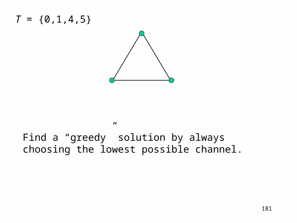
181

Find a “greedy” solution by always choosing the lowest possible channel.

T = {0,1,4,5}

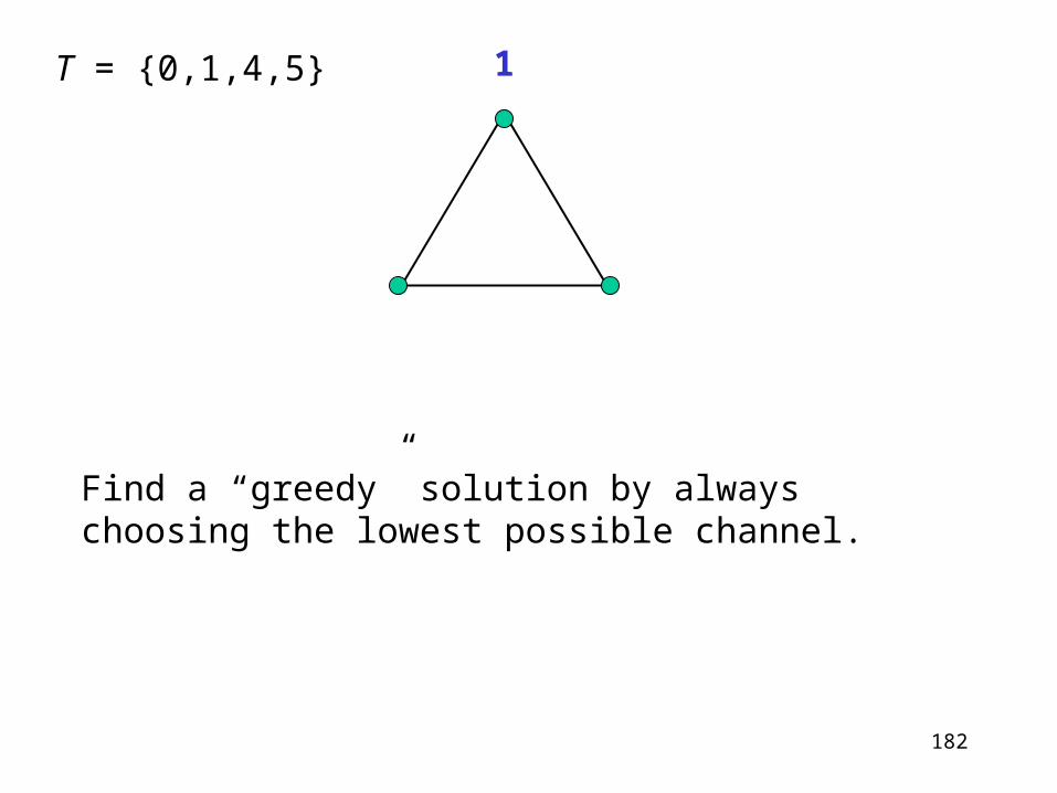
182

1

Find a “greedy” solution by always choosing the lowest possible channel.

T = {0,1,4,5}

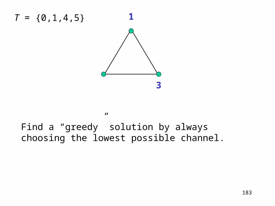
183

1

3

Find a “greedy” solution by always choosing the lowest possible channel.

T = {0,1,4,5}

184

1

9 3

Find a “greedy” solution by always choosing the lowest possible channel.

T = {0,1,4,5}

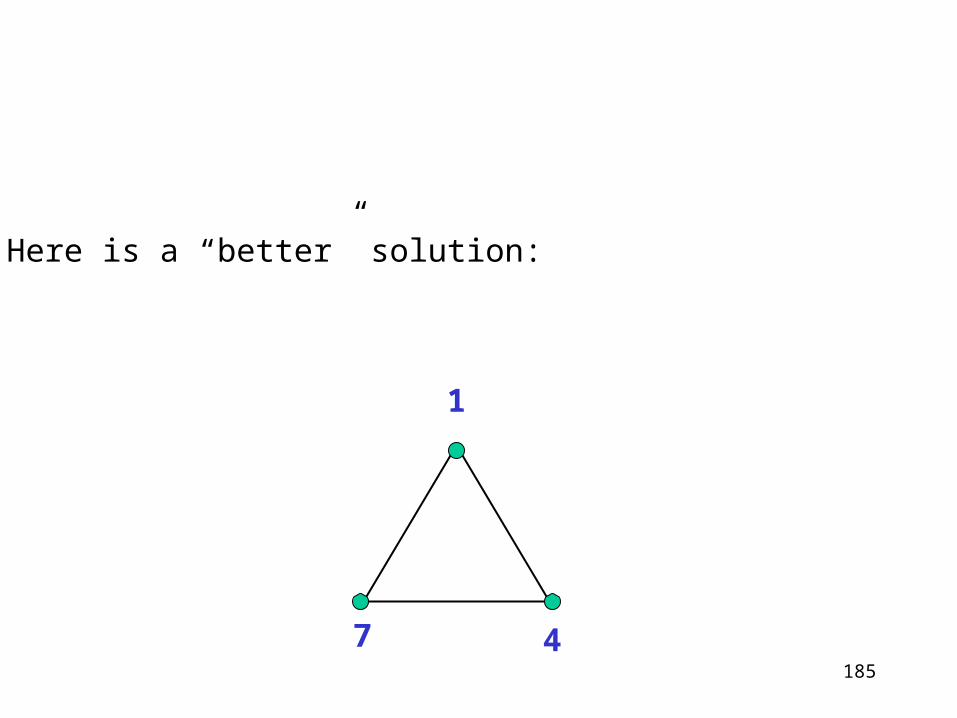
185

1

7 4

Here is a “better” solution:

186

In what sense is this better? In the sense that

is smaller.

S(f) is called the span of f.

The minimum S(f) over all T-colorings f of G is called the span of G.

(Note that it is NP-complete to compute the optimal span.)

Widely studied question: For what graphs does the greedy algorithm obtain the optimal span?

S(f ) = maxx;y2V

jf (x) ¡ f (y)j

187

What if numbers in T change by a scale transformation? Is the answer to this widely studied question meaningful?

Consider the case of ratio scales. Then we can have transformations t t, > 0.

In this case, even for complete graphs Kn, the conclusion that the greedy algorithm obtains the optimal span is meaningless.

Take the above example with = 2. Then

T = {0,2,8,10}

The greedy algorithm does obtain the optimal span:

188

1

T = {0,2,8,10}

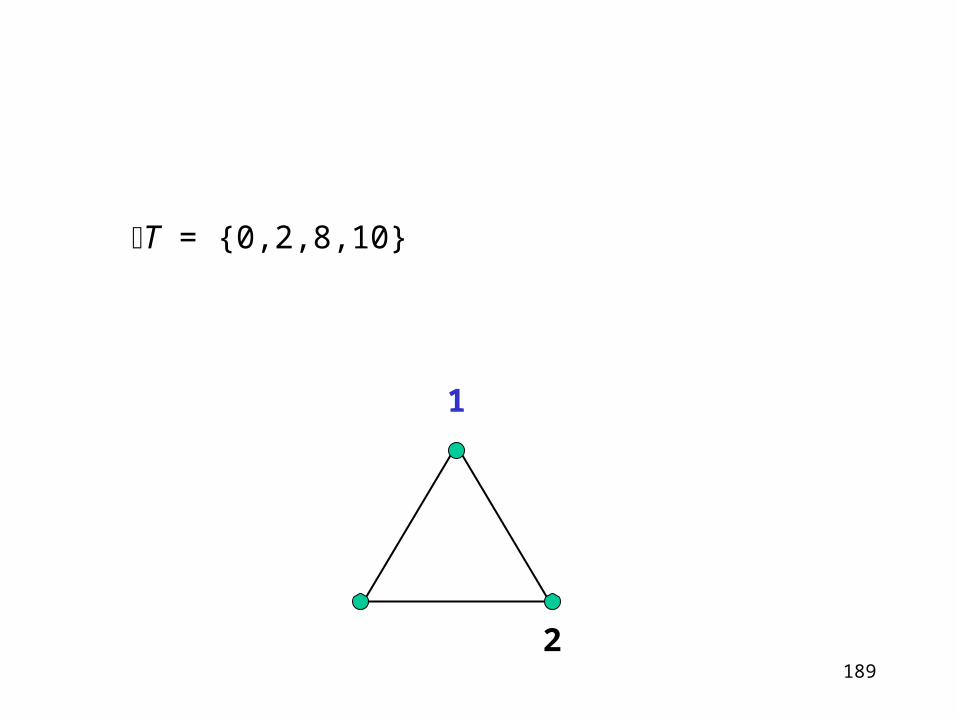
189

1

2

T = {0,2,8,10}

190

1

5 2

T = {0,2,8,10}

191

Aside

It is not as easy to give an example of a complete graph Kn and set T and number such that the greedy algorithm obtains the optimal span for Kn with T but not with T.

One example is K6 with

and = 2.

The greedy T-coloring uses the channels 1, 6, 15, 20, 29, 34.

T = f0;1;2;3;4g[ f8g[ f10;11;12g[ f31;32g

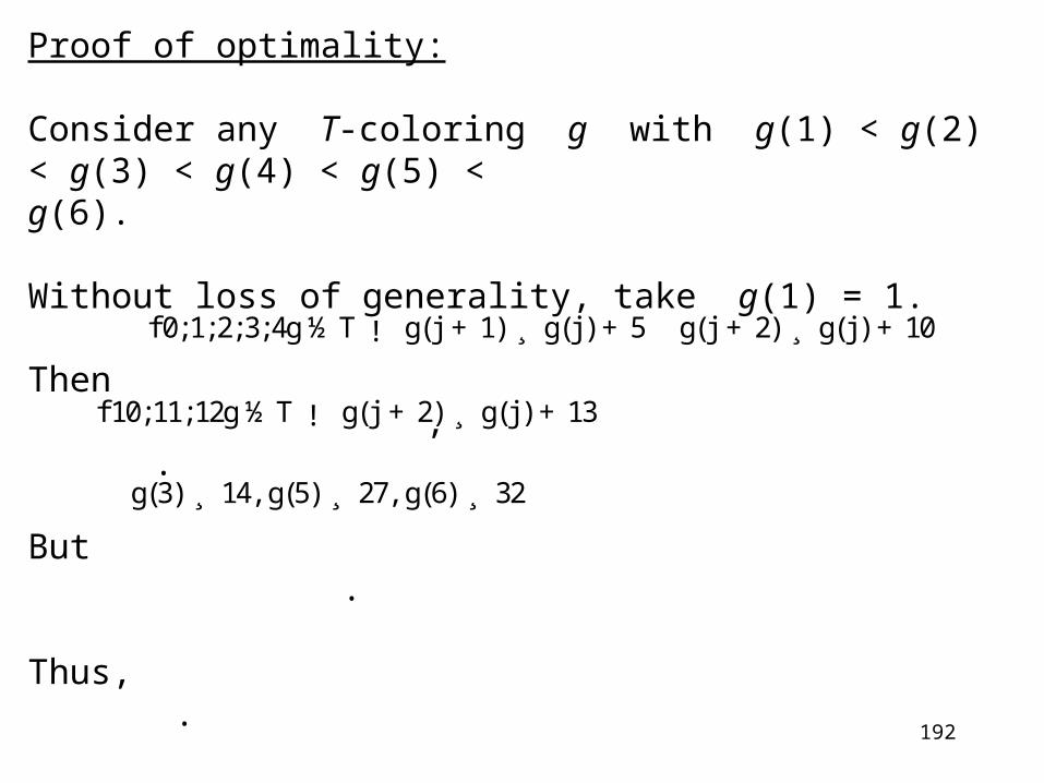
192

Proof of optimality:

Consider any T-coloring g with g(1) < g(2) < g(3) < g(4) < g(5) < g(6).

Without loss of generality, take g(1) = 1.

Then , .

But .

Thus, .

But 32-1 = 31, 33-1 = 32, so g(6) 34.

QED

g(j +2) ¸ g(j ) +10

g(3) ¸ 14, g(5) ¸ 27, g(6) ¸ 32

f0;1;2;3;4g½T ! g(j +1) ¸ g(j ) +5

f10;11;12g½T ! g(j +2) ¸ g(j ) +13

193

With = 2,

The greedy T-coloring uses the channels 1, 2, 11, 12, 29, 30.

A better T-coloring uses the channels 1, 2, 13, 14, 27, 28.

®T = f0;2;4;6;8g[ f16g[ f20;22;24g[ f62;64g:

194

What is meaningful?

Theorem (Cozzens and Roberts 1991): The conclusion that the greedy algorithm obtains the optimal span for all complete graphs is meaningful if elements of T are measured on a ratio scale.

For example, if T = {0,1,2, ... , r}, this conclusion is true for all complete graphs. Even true if T = {0,1,2, ..., r} S where S contains no multiple of r+1.

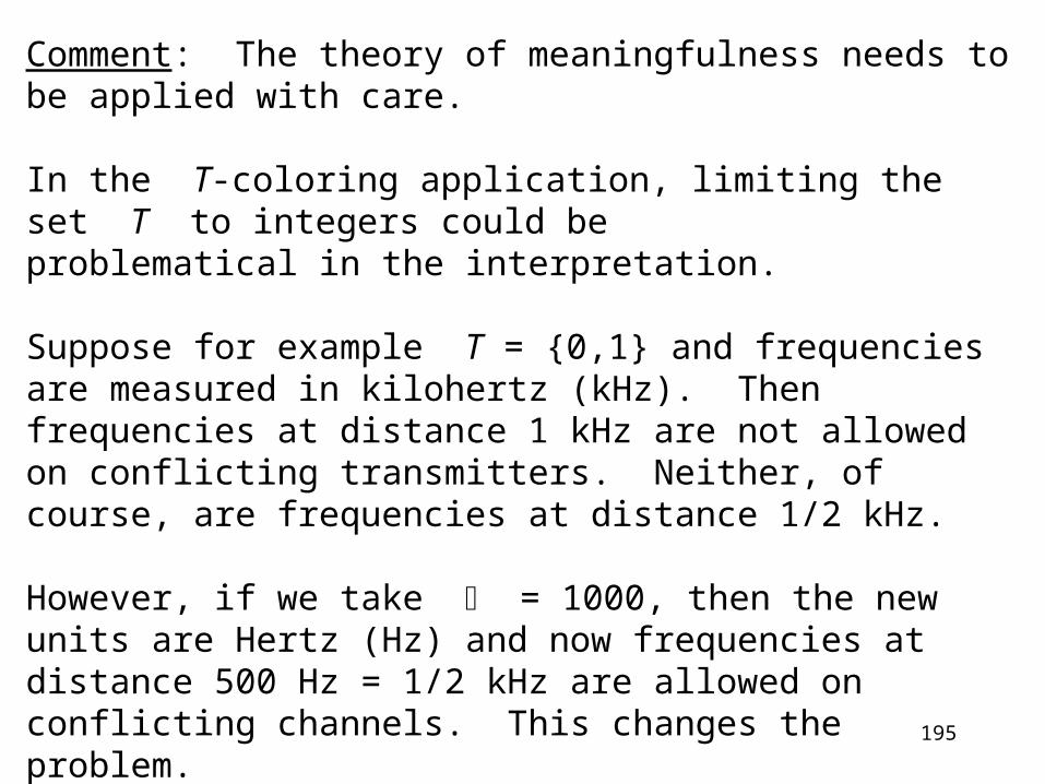
195

Comment: The theory of meaningfulness needs to be applied with care.

In the T-coloring application, limiting the set T to integers could be problematical in the interpretation.

Suppose for example T = {0,1} and frequencies are measured in kilohertz (kHz). Then frequencies at distance 1 kHz are not allowed on conflicting transmitters. Neither, of course, are frequencies at distance 1/2 kHz.

However, if we take = 1000, then the new units are Hertz (Hz) and now frequencies at distance 500 Hz = 1/2 kHz are allowed on conflicting channels. This changes the problem.

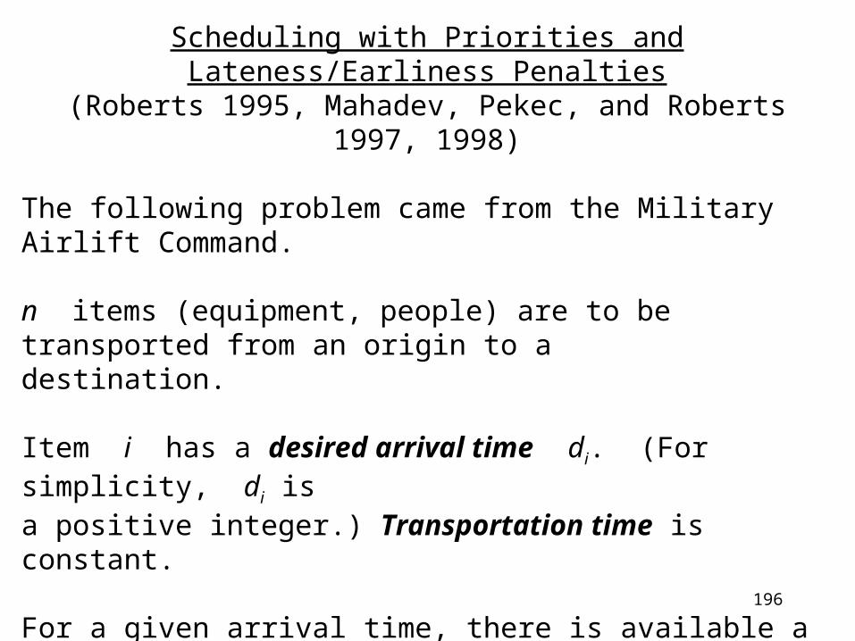
196

Scheduling with Priorities and Lateness/Earliness Penalties(Roberts 1995, Mahadev, Pekec, and Roberts 1997, 1998)

The following problem came from the Military Airlift Command.

n items (equipment, people) are to be transported from an origin to a destination.

Item i has a desired arrival time di. (For simplicity, di isa positive integer.) Transportation time is constant.

For a given arrival time, there is available a certain capacity c for transportation (# of seats, cargo space, etc.) Note constant c.

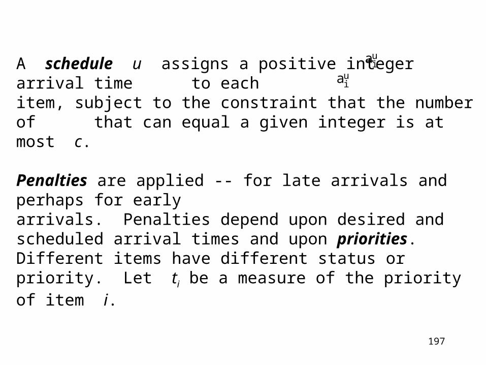
197

A schedule u assigns a positive integer arrival time to each item, subject to the constraint that the number of that can equal a given integer is at most c.

Penalties are applied -- for late arrivals and perhaps for early arrivals. Penalties depend upon desired and scheduled arrival times and upon priorities. Different items have different status or priority. Let ti be a measure of the priority of item i.

auiaui

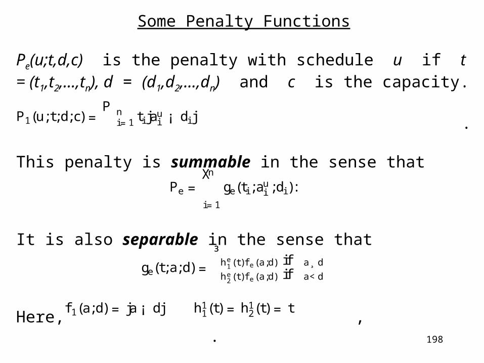
198

Some Penalty Functions

Pe(u;t,d,c) is the penalty with schedule u if t = (t1,t2,...,tn), d = (d1,d2,...,dn) and c is the capacity.

.

This penalty is summable in the sense that

It is also separable in the sense that

Here, , .

P1(u;t;d;c) =P n

i=1ti jaui ¡ di j

Pe =nX

i=1

ge(ti ;aui ;di ):

ge(t;a;d) =³he1(t)f e(a;d) if a¸ d

he2(t)f e(a;d) if a<d

f 1(a;d) = ja¡ dj h11(t) = h12(t) = t

199

Other examples of summable, separable penalty functions have and fe(a,d) defined as follows:

if a > d and 0 otherwise.

if a d and 0 otherwise.

if a d and |a - d| otherwise

A summable example is P6(u;t,d,c): g6(t,a,d) = 1 if a d + F(t) and 0 otherwise.

he1(t) = he2(t) = t

P2(u;t;d;c) : f 2(a;d) = ja¡ dj

P3(u;t;d;c) : f 3(a;d) = 1

P4(u;t;d;c) : f 4(a;d) = °ja¡ dj

P5(u;t;d;c) : f 5(a;d) = ja¡ dj2

200

Problem: Find an optimal schedule, i.e., one which minimizes the penalty.

Analogous Problem in Manufacturing

n tasks to perform;task i has desired completion time di;c processors;constant processing time;tasks have different priorities

This problem arises in "just-in-time" production: Toyota, Boeing, etc.

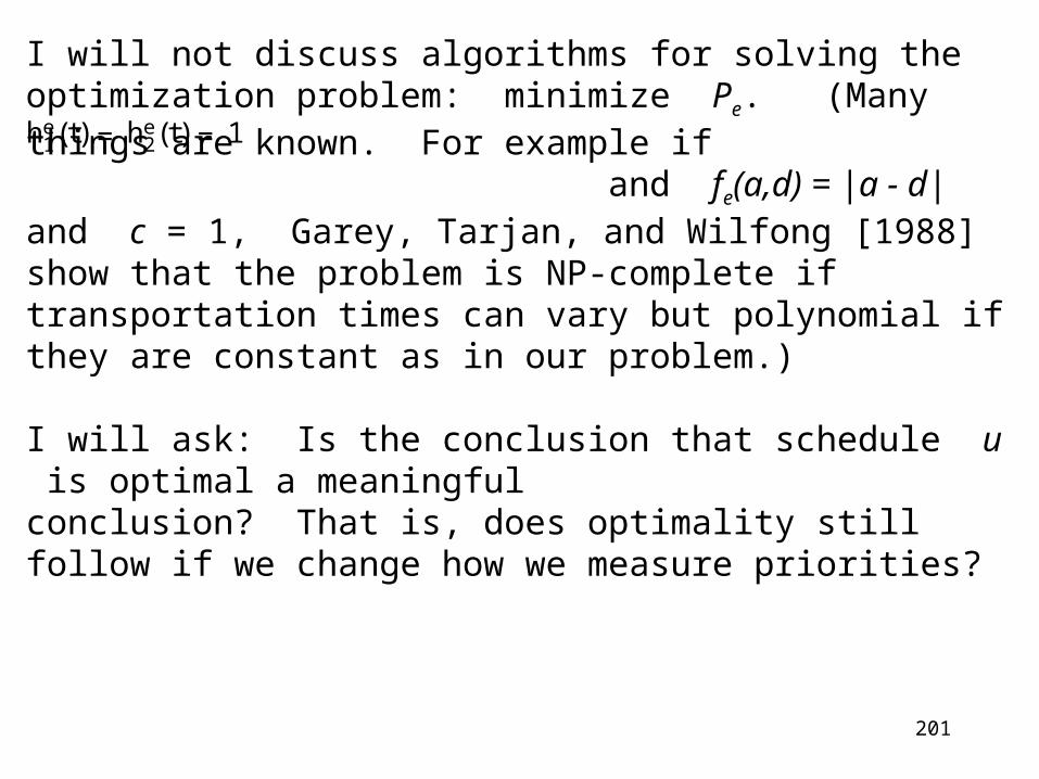
201

I will not discuss algorithms for solving the optimization problem: minimize Pe. (Many things are known. For example if and fe(a,d) = |a - d| and c = 1, Garey, Tarjan, and Wilfong [1988] show that the problem is NP-complete if transportation times can vary but polynomial if they are constant as in our problem.)

I will ask: Is the conclusion that schedule u is optimal a meaningful conclusion? That is, does optimality still follow if we change how we measure priorities?

he1(t) = he2(t) = 1

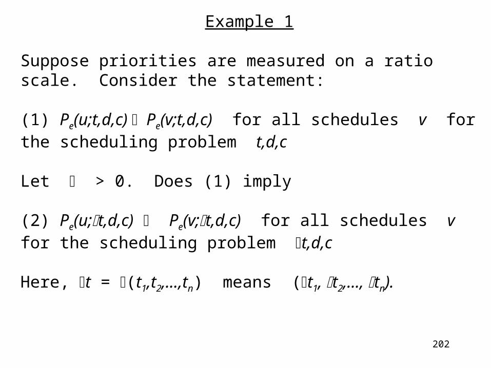
202

Example 1

Suppose priorities are measured on a ratio scale. Consider the statement:

(1) Pe(u;t,d,c) Pe(v;t,d,c) for all schedules v for the scheduling problem t,d,c

Let > 0. Does (1) imply

(2) Pe(u;t,d,c) Pe(v;t,d,c) for all schedules v for the scheduling problem t,d,c

Here, t = (t1,t2,...,tn) means (t1, t2,..., tn).

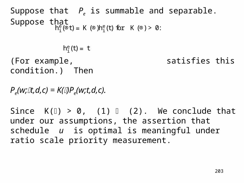
203

Suppose that Pe is summable and separable. Suppose that

(For example, satisfies this condition.) Then

Pe(w;t,d,c) = K()Pe(w;t,d,c).

Since K() > 0, (1) (2). We conclude that under our assumptions, the assertion that schedule u is optimal is meaningful under ratio scale priority measurement.

hei (®t) = K (®)hei (t) for K (®) > 0:

hei (t) = t

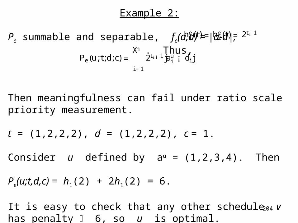
204

Example 2:

Pe summable and separable, fe(a,d) = |a-d|, . Thus,

Then meaningfulness can fail under ratio scale priority measurement.

t = (1,2,2,2), d = (1,2,2,2), c = 1.

Consider u defined by au = (1,2,3,4). Then

Pe(u;t,d,c) = h1(2) + 2h1(2) = 6.

It is easy to check that any other schedule v has penalty 6, so u is optimal.

he1(t) = he2(t) = 2t¡ 1

Pe(u;t;d;c) =nX

i=1

2ti ¡ 1jaui ¡ di j

205

However, consider = 2. Then t = (2,4,4,4).

Pe(u;2t,d,c) = h1(4) + 2h1(4) = 24.

Let av be given by (4,1,2,3). Then

Pe(v;2t,d,c) = 3h1(2) + h2(4) + h1(4) = 22.

Thus, u is no longer optimal after a change of unit.

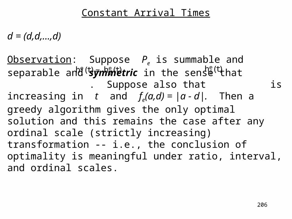
206

Constant Arrival Times

d = (d,d,...,d)

Observation: Suppose Pe is summable and separable and symmetric in the sense that . Suppose also that is increasing in t and fe(a,d) = |a - d|. Then a greedy algorithm gives the only optimal solution and this remains the case after any ordinal scale (strictly increasing) transformation -- i.e., the conclusion of optimality is meaningful under ratio, interval, and ordinal scales.

he1(t) = he2(t) hei (t)

207

Example 3

The conclusion we have stated is false without symmetry.

fe(a,d) = |a - d|

t = (1/4,1/9,1), d = (2,2,2), c = 1.

Then the optimal schedule u is given by au = (3,4,2).

.

he1(t) = t2, he2(t) =pt

Pe(u;t;d;c) = he1(1=4) +2he1(1=9) = 1=16+2=81

208

In comparison, if av = (3,1,2), then

.

However, let = 36. Then t = (9,4,36) and

.

.

Thus, u is no longer optimal.

Pe(v;t;d;c) = he1(1=4) +he2(1=9) = 1=16+1=3

Pe(u;®t;d;c) = he1(9) +2he1(4) = 81+32

Pe(v;®t;d;c) = he1(9) +he2(4) = 81+2

209

Nonconstant Arrival Times

Observation: Suppose , fe(a,d) = |a - d|.

As noted above in Example 1, optimality is meaningful for ratio scale priority measurement with this penalty function. However, we note that it fails for interval scale priority measurement. Are interval scales relevant to priority measurement in scheduling? Yes. Utility or worth or loss of goodwill are not necessarily ratio scales and could very well be interval or ordinal scales.

t = (9,9,9,1), d = (2,2,2,1), c = 1.

au = (2,1,3,4); Pe(u;t,d,c) = 21.

It is easy to check that u is optimal.

he1(t) = he2(t) = t

210

However, let = 1/8, = 7/8. Then t+ = (2,2,2,1) and

Pe(u; t+,d,c) = 7.

If av = (2,3,4,1), then

Pe(v; t+,d,c) = 6.

211

A Special Case of Interval Scale Priority Measurement and Nonconstant d

Assumptions:

Let d = (d,d,...,d,k), with 0 < d < k n. Let c = 1.

Suppose Pe is summable and separable with increasing in t, i = 1,2, and with fe(a,d) = D|a - d|, D > 0.

Assume that

Theorem: Then the conclusion that u is an optimal schedule is meaningful if priorities are measured on an interval scale.

hei (t)

hei (®t+¯) = K (®;¯)hei (t) +L(®;¯);

K (®;¯) > 0: