1 Logistic Regression Source This note follows Business Research Methods and Statistics using SPSS...
36
1 Logistic Regression Source This note follows Business Research Methods and Statistics using SPSS by Robert Burns & Richard Burns (text) for which it is an additional chapter (24) . Saturday 12 March 2022 02:26 PM
-
Upload
emerald-chandler -
Category
Documents
-
view
257 -
download
2
Transcript of 1 Logistic Regression Source This note follows Business Research Methods and Statistics using SPSS...

1
Logistic Regression
Source
This note follows Business Research Methods and Statistics using SPSS by Robert Burns & Richard Burns (text) for which it is an additional chapter (24).
Wednesday 19 April 2023 12:34 AM
2
Logistic Regression
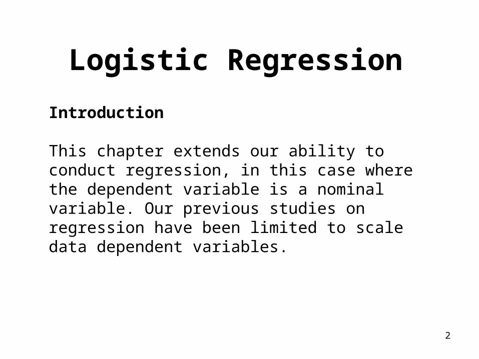
Introduction
This chapter extends our ability to conduct regression, in this case where the dependent variable is a nominal variable. Our previous studies on regression have been limited to scale data dependent variables.
3
Logistic Regression
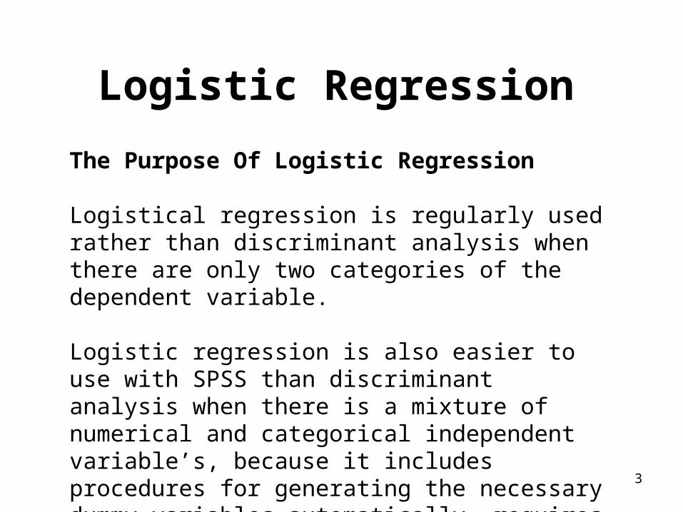
The Purpose Of Logistic Regression
Logistical regression is regularly used rather than discriminant analysis when there are only two categories of the dependent variable.
Logistic regression is also easier to use with SPSS than discriminant analysis when there is a mixture of numerical and categorical independent variable’s, because it includes procedures for generating the necessary dummy variables automatically, requires fewer assumptions, and is more statistically robust.

4
Logistic Regression
The Purpose Of Logistic Regression
Since the dependent variable is dichotomous we cannot predict a numerical value for it using logistic regression, so the usual regression least squares deviations criteria for best fit approach of minimizing error around the line of best fit is inappropriate. Logistic regression forms a best fitting equation or function using the maximum likelihood method.

5
Logistic Regression
The Purpose Of Logistic Regression
Like ordinary regression, logistic regression provides a coefficient, which measures each independent variable’s partial contribution to variations in the dependent variable. The goal is to correctly predict the category of outcome for individual cases using the most parsimonious model.

6
Logistic Regression
There are two main uses of logistic regression:
The first is the prediction of group membership.
Logistic regression also provides knowledge of the relationships and strengths among the variables (e.g. marrying the boss’s daughter puts you at a higher probability for job promotion than undertaking five hours unpaid overtime each week).

7
Assumptions Of Logistic Regression
1. Logistic regression does not assume a linear relationship between the dependent and independent variables.
2. The dependent variable must be a dichotomy (2 categories).
3. The independent variables need not be interval, nor normally distributed, nor linearly related, nor of equal variance within each group.

8
Logistic Regression
For those interested the printed notes contain more technical details.

9
Data - Logistic Regression
The data file contains data from a survey of home owners conducted by an electricity company about an offer of roof solar panels with a 50% subsidy from the state government as part of the state’s environmental policy. The variables involve household income measured in units of a thousand dollars, age, monthly mortgage, size of family household, and whether the householder would take or decline the offer. You can follow the instructions below and conduct a logistic regression to determine whether family size and monthly mortgage will predict taking or declining the offer.

10
Data - Logistic Regression
Acronym Description
income household income in $,000
age years old
takeoffer take solar panel offer {0 decline offer}
Mortgage monthly mortgage payment
Famsize number of persons in household
n = 30
11
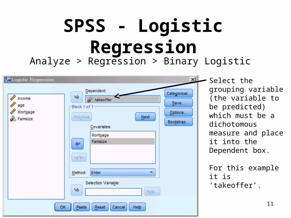
SPSS - Logistic Regression
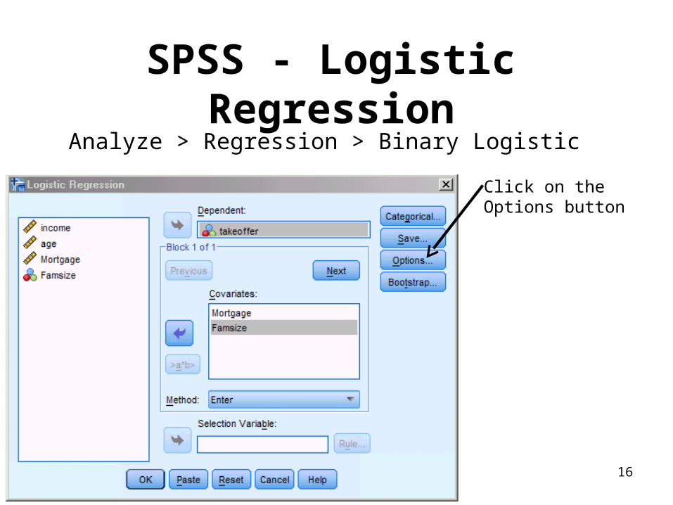
Analyze > Regression > Binary Logistic
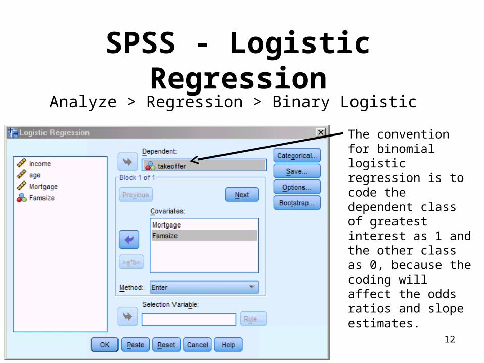
Select the grouping variable (the variable to be predicted) which must be a dichotomous measure and place it into the Dependent box.
For this example it is ‘takeoffer’.
12
SPSS - Logistic Regression
Analyze > Regression > Binary Logistic
The convention for binomial logistic regression is to code the dependent class of greatest interest as 1 and the other class as 0, because the coding will affect the odds ratios and slope estimates.
13
SPSS - Logistic Regression
Analyze > Regression > Binary Logistic
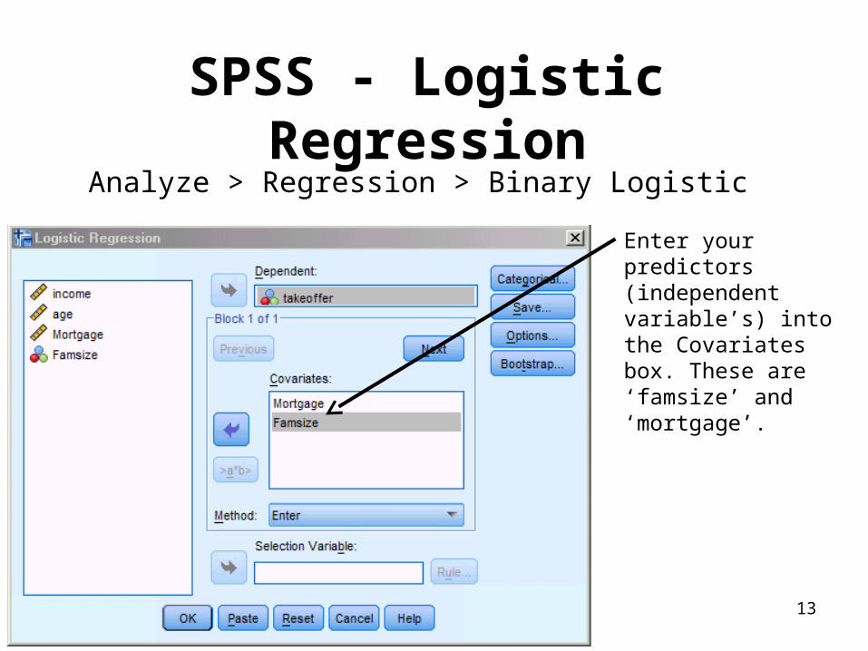
Enter your predictors (independent variable’s) into the Covariates box. These are ‘famsize’ and ‘mortgage’.
14
SPSS - Logistic Regression
Analyze > Regression > Binary Logistic
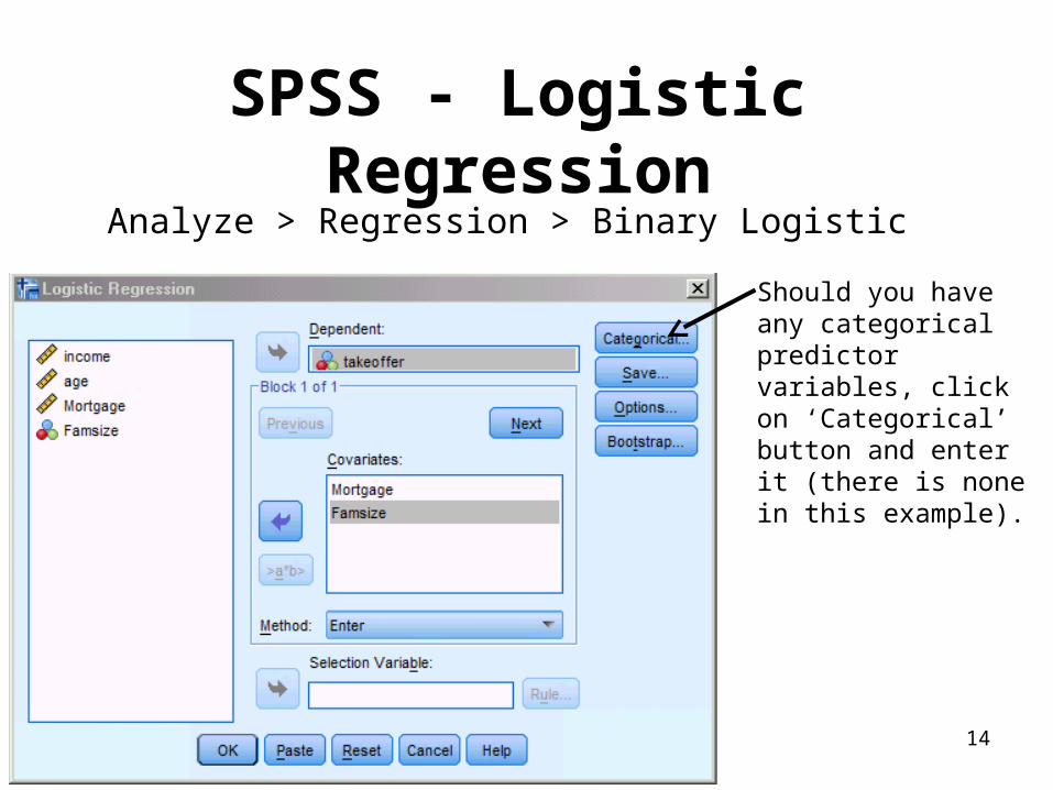
Should you have any categorical predictor variables, click on ‘Categorical’ button and enter it (there is none in this example).
15
SPSS - Logistic Regression
Analyze > Regression > Binary Logistic
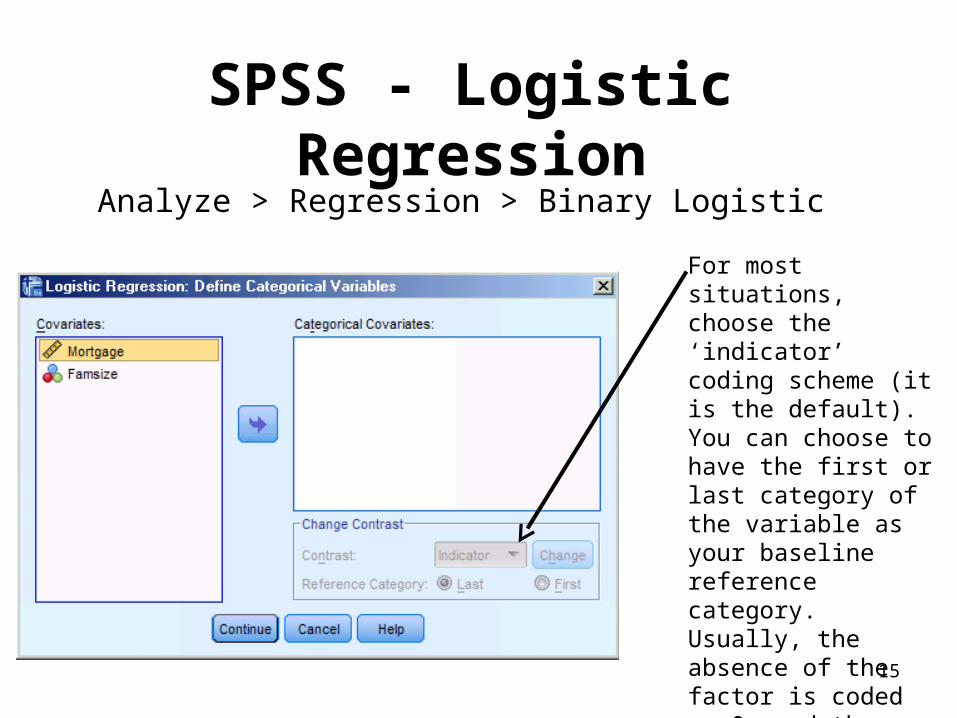
For most situations, choose the ‘indicator’ coding scheme (it is the default). You can choose to have the first or last category of the variable as your baseline reference category. Usually, the absence of the factor is coded as 0, and the presence of the factor is coded 1.
16
SPSS - Logistic Regression
Analyze > Regression > Binary Logistic
Click on the Options button
17
SPSS - Logistic Regression
Analyze > Regression > Binary Logistic
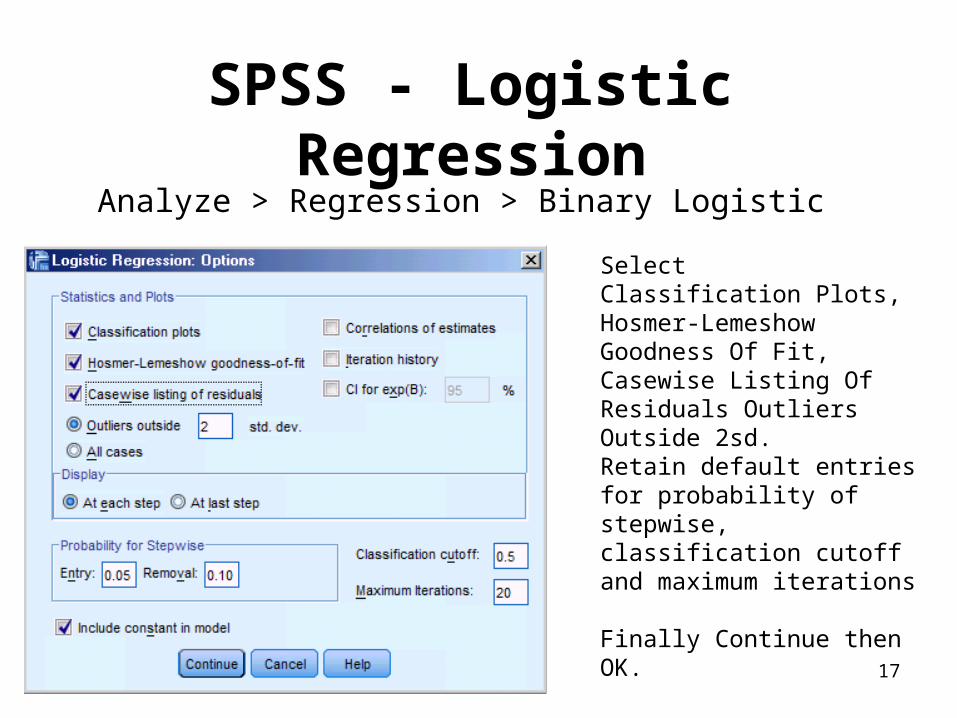
Select Classification Plots, Hosmer-Lemeshow Goodness Of Fit, Casewise Listing Of Residuals Outliers Outside 2sd. Retain default entries for probability of stepwise, classification cutoff and maximum iterations
Finally Continue then OK.

18
Interpretation Of The Output
Presents the results with only the constant included before any coefficients (i.e. those relating to family size and mortgage) are entered into the equation. Logistic regression compares this model with a model including all the predictors (family size and mortgage) to determine whether the latter model is more appropriate. The table suggests that if we knew nothing about our variables and guessed that a person would not take the offer we would be correct 53.3% of the time.
Block 0: Beginning Block
Classification Tablea,b
Predicted
takeoffer
Observed .00 1.00
Percentage
Correct
.00 0 14 .0 takeoffer
1.00 0 16 100.0
Step 0
Overall Percentage 53.3
a. Constant is included in the model.
b. The cut value is .500

19
Interpretation Of The Output
The table tells us whether each independent variable improves the model. The answer is yes for both variables, with family size slightly better than mortgage size, as both are significant and if included would add to the predictive power of the model. If they had not been significant and able to contribute to the prediction, then termination of the analysis would obviously occur at this point.
Variables not in the Equation
Score df Sig.
Mortgage 6.520 1 .011 Variables
Famsize 14.632 1 .000
Step 0
Overall Statistics 15.085 2 .001

20
Interpretation Of The Output
The classification error rate has changed from the original 53.3% (slide 18). By adding the variables we can now predict with 90% accuracy. The model appears good, but we need to evaluate model fit and significance as well. SPSS will offer you a variety of statistical tests for model fit and whether each of the independent variables included make a significant contribution to the model.
Classification Tablea
Predicted
takeoffer
Observed .00 1.00
Percentage
Correct
.00 13 1 92.9 takeoffer
1.00 2 14 87.5
Step 1
Overall Percentage 90.0
a. The cut value is .500

21
Interpretation Of The Output
The overall significance is tested using what SPSS calls the Model Chi square, which is derived from the likelihood of observing the actual data under the assumption that the model that has been fitted is accurate. There are two hypotheses to test in relation to the overall fit of the model:
H0 The model is a good fitting model.H1 The model is not a good fitting model (i.e. the predictors have a significant effect).

22
Interpretation Of The Output
The difference between –2log likelihood for the best-fitting model and –2log likelihood for the null hypothesis model (in which all the b values are set to zero in block 0) is distributed like chi squared, with degrees of freedom equal to the number of predictors; this difference is the Model chi square that SPSS refers to The –2log likelihood value from the Model Summary table is 17.359.
Model Summary
Step
-2 Log
likelihood
Cox & Snell R
Square
Nagelkerke R
Square
1 17.359a .552 .737
a. Estimation terminated at iteration number 8 because
parameter estimates changed by less than .001.
23
Interpretation Of The Output
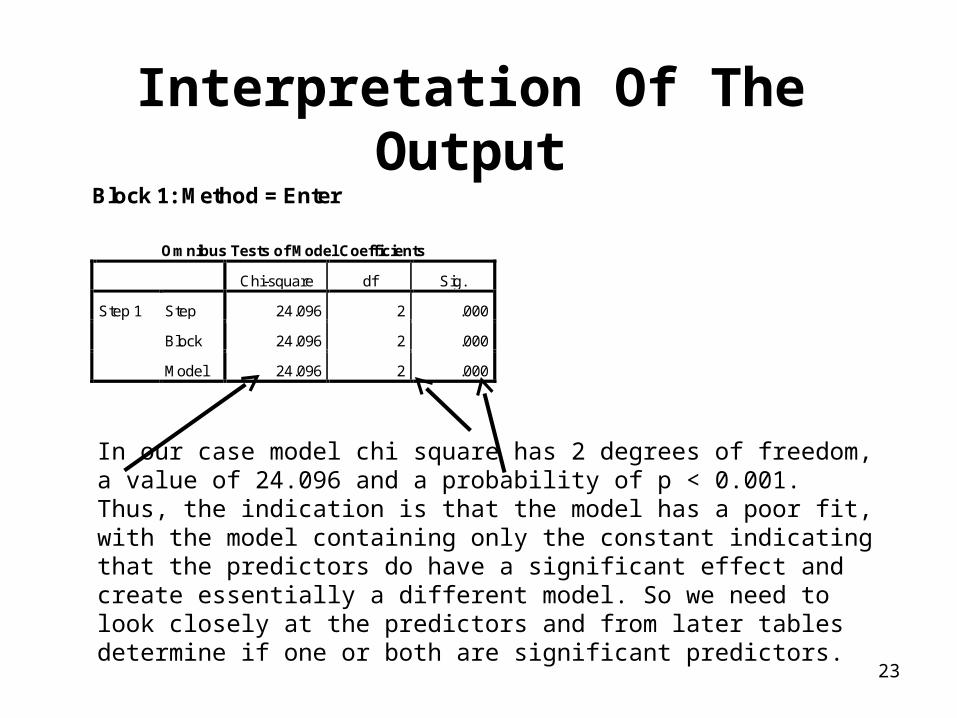
In our case model chi square has 2 degrees of freedom, a value of 24.096 and a probability of p < 0.001. Thus, the indication is that the model has a poor fit, with the model containing only the constant indicating that the predictors do have a significant effect and create essentially a different model. So we need to look closely at the predictors and from later tables determine if one or both are significant predictors.
Block 1: Method = Enter
Omnibus Tests of Model Coefficients
Chi-square df Sig.
Step 1 Step 24.096 2 .000
Block 24.096 2 .000
Model 24.096 2 .000

24
Interpretation Of The Output
Although there is no close analogous statistic in logistic regression to the coefficient of determination R2 the Model Summary Table provides some approximations. Cox and Snell’s R-Square attempts to imitate multiple R-Square based on ‘likelihood’, but its maximum can be (and usually is) less than 1.0, making it difficult to interpret. Here it is indicating that 55.2% of the variation in the dependent variable is explained by the logistic model. The Nagelkerke modification that does range from 0 to 1 is a more reliable measure of the relationship. Nagelkerke’s R2 will normally be higher than the Cox and Snell measure. Nagelkerke’s R2 is part of SPSS output in the ‘Model Summary’ table and is the most-reported of the R-squared estimates. In our case it is 0.737, indicating a moderately strong relationship of 73.7% between the predictors and the prediction.
25
Interpretation Of The Output
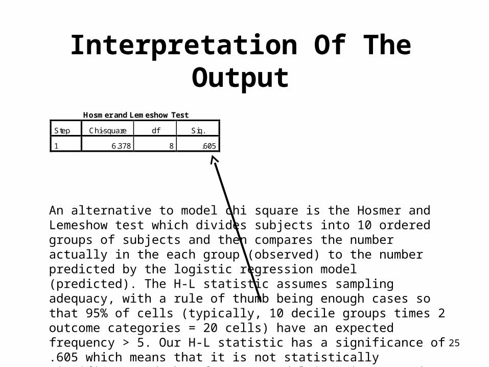
An alternative to model chi square is the Hosmer and Lemeshow test which divides subjects into 10 ordered groups of subjects and then compares the number actually in the each group (observed) to the number predicted by the logistic regression model (predicted). The H-L statistic assumes sampling adequacy, with a rule of thumb being enough cases so that 95% of cells (typically, 10 decile groups times 2 outcome categories = 20 cells) have an expected frequency > 5. Our H-L statistic has a significance of .605 which means that it is not statistically significant and therefore our model is quite a good fit.
Hosmer and Lemeshow Test
Step Chi-square df Sig.
1 6.378 8 .605
26
Interpretation Of The Output
Rather than using a goodness-of-fit statistic, we often want to look at the proportion of cases we have managed to classify correctly. For this we need to look at the classification table printed out by SPSS, which tells us how many of the cases where the observed values of the dependent variable were 1 or 0 respectively have been correctly predicted. In the Classification table, the columns are the two predicted values of the dependent, while the rows are the two observed (actual) values of the dependent. In a perfect model, all cases will be on the diagonal and the overall percent correct will be 100%.
27
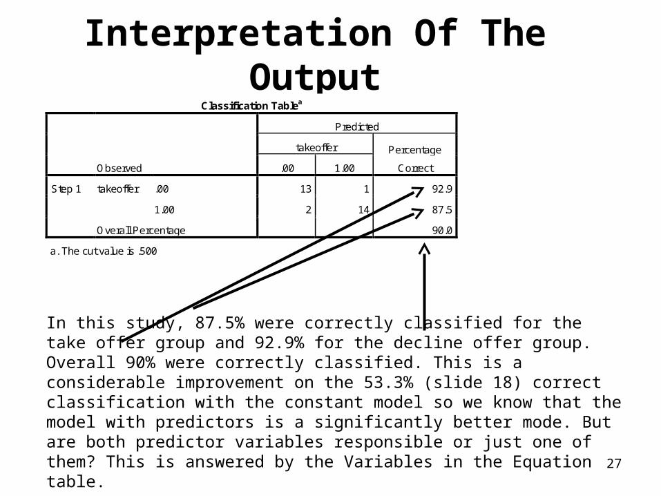
Interpretation Of The Output
In this study, 87.5% were correctly classified for the take offer group and 92.9% for the decline offer group. Overall 90% were correctly classified. This is a considerable improvement on the 53.3% (slide 18) correct classification with the constant model so we know that the model with predictors is a significantly better mode. But are both predictor variables responsible or just one of them? This is answered by the Variables in the Equation table.
Classification Tablea
Observed
Predicted
takeoffer Percentage
Correct .00 1.00
Step 1 takeoffer .00 13 1 92.9
1.00 2 14 87.5
Overall Percentage 90.0
a. The cut value is .500

28
Interpretation Of The Output
The Variables in the Equation table has several important elements. The Wald statistic and associated probabilities provide an index of the significance of each predictor in the equation. The Wald statistic has a chi-square distribution.
The simplest way to assess Wald is to take the significance values and if less than .05 reject the null hypothesis as the variable does make a significant contribution. In this case, we note that family size contributed significantly to the prediction (p = .013) but mortgage did not (p = .075). The researcher may well want to drop independents from the model when their effect is not significant by the Wald statistic (in this case mortgage).
Variables in the Equation
B S.E. Wald df Sig. Exp(B)
Mortgage .005 .003 3.176 1 .075 1.005
Famsize 2.399 .962 6.215 1 .013 11.007
Step 1a
Constant -18.627 8.654 4.633 1 .031 .000
a. Variable(s) entered on step 1: Mortgage, Famsize.

29
Interpretation Of The Output
The Exp(B) column in the table presents the extent to which raising the corresponding measure by one unit influences the odds ratio. We can interpret Exp(B) in terms of the change in odds. If the value exceeds 1 then the odds of an outcome occurring increase; if the figure is less than 1, any increase in the predictor leads to a drop in the odds of the outcome occurring. For example, the Exp(B) value associated with family size is 11.007. Hence when family size is raised by one unit (one person) the odds ratio is 11 times as large and therefore householders are 11 more times likely to belong to the take offer group.
Variables in the Equation
B S.E. Wald df Sig. Exp(B)
Mortgage .005 .003 3.176 1 .075 1.005
Famsize 2.399 .962 6.215 1 .013 11.007
Step 1a
Constant -18.627 8.654 4.633 1 .031 .000
a. Variable(s) entered on step 1: Mortgage, Famsize.

30
Interpretation Of The Output
The ‘B’ values are the logistic coefficients that can be used to create a predictive equation (similar to the b values in linear regression) formula. In this example:
Variables in the Equation
B S.E. Wald df Sig. Exp(B)
Mortgage .005 .003 3.176 1 .075 1.005
Famsize 2.399 .962 6.215 1 .013 11.007
Step 1a
Constant -18.627 8.654 4.633 1 .031 .000
a. Variable(s) entered on step 1: Mortgage, Famsize.
62718mortgage0050sizeamily 3992
62718mortgage0050sizeamily 3992
1case a ofy Probabilit
..f.
..f.
e
e
31
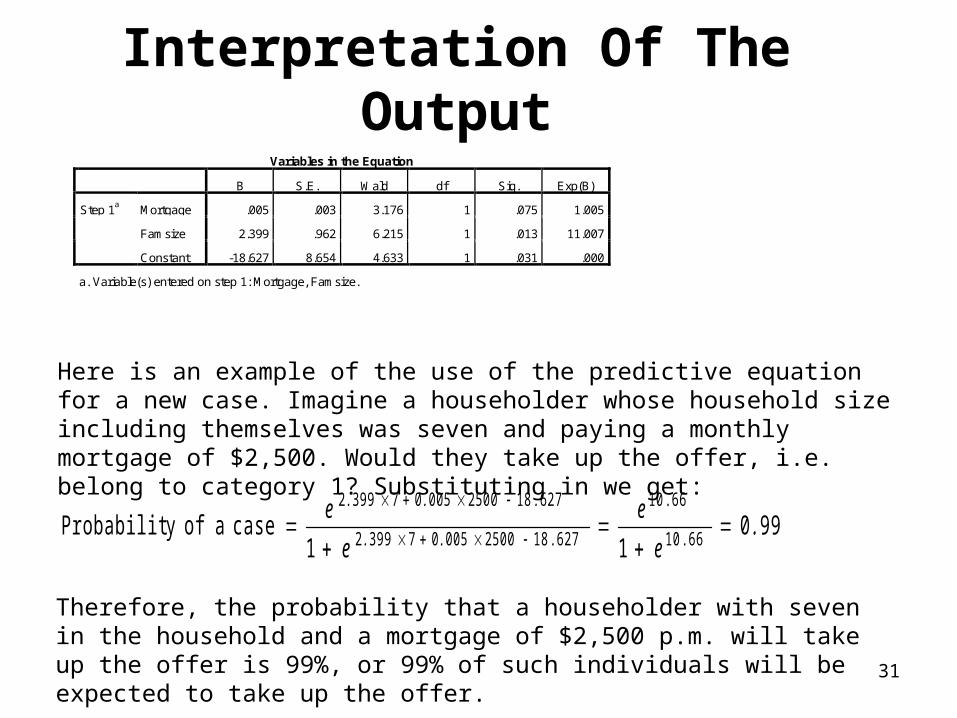
Interpretation Of The Output
Here is an example of the use of the predictive equation for a new case. Imagine a householder whose household size including themselves was seven and paying a monthly mortgage of $2,500. Would they take up the offer, i.e. belong to category 1? Substituting in we get:
Variables in the Equation
B S.E. Wald df Sig. Exp(B)
Mortgage .005 .003 3.176 1 .075 1.005
Famsize 2.399 .962 6.215 1 .013 11.007
Step 1a
Constant -18.627 8.654 4.633 1 .031 .000
a. Variable(s) entered on step 1: Mortgage, Famsize.
99011
case a ofy Probabilit6610
6610
627182500005073992
627182500005073992
.e
e
e
e.
.
...
...
Therefore, the probability that a householder with seven in the household and a mortgage of $2,500 p.m. will take up the offer is 99%, or 99% of such individuals will be expected to take up the offer.

32
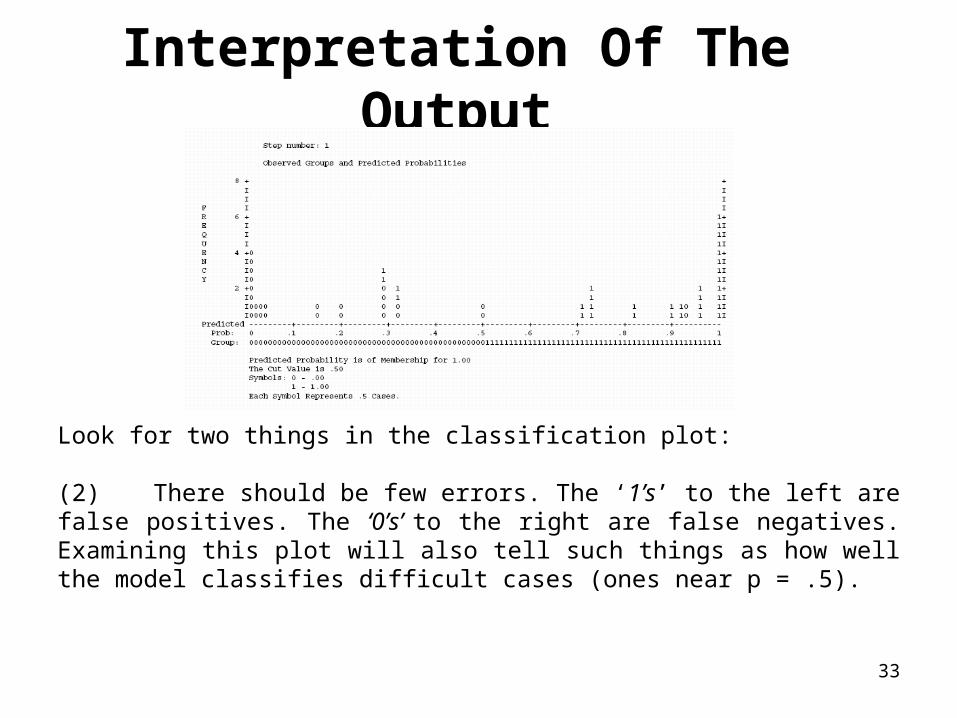
Interpretation Of The Output
Look for two things in the classification plot: (1) A U-shaped rather than normal distribution is desirable. A U-shaped distribution indicates the predictions are well-differentiated with cases clustered at each end showing correct classification. A normal distribution indicates too many predictions close to the cut point, with a consequence of increased misclassification around the cut point which is not a good model fit. For these around .50 you could just as well toss a coin.
33
Interpretation Of The Output
Look for two things in the classification plot: (2) There should be few errors. The ‘1’s’ to the left are false positives. The ‘0’s’ to the right are false negatives. Examining this plot will also tell such things as how well the model classifies difficult cases (ones near p = .5).

34
Interpretation Of The Output
Finally, the casewise list produces a list of cases that didn’t fit the model well. These are outliers. If there are a number of cases this may reveal the need for further explanatory variables to be added to the model. Only one case (No. 21) falls into this category in our example and therefore the model is reasonably sound. This is the only person who did not fit the general pattern. We do not expect to obtain a perfect match between observation and prediction across a large number of cases. No excessive outliers should be retained as they can affect results significantly. The researcher should inspect standardized residuals for outliers (ZResid) and consider removing them if they exceed > 2.58 (outliers at the .01 level).
Casewise Listb
Observed Temporary Variable
Case
Selected
Statusa takeoffer Predicted Predicted Group Resid ZResid
21 S 0** .924 1 -.924 -3.483
a. S = Selected, U = Unselected cases, and ** = Misclassified cases.
b. Cases with studentized residuals greater than 2.000 are listed.
35
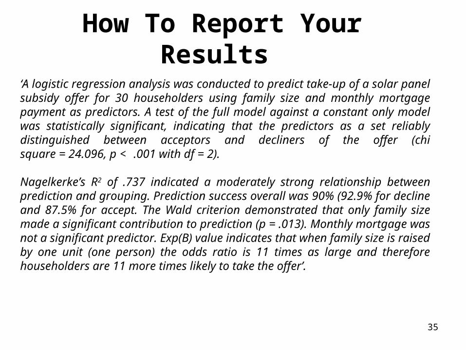
How To Report Your Results
‘A logistic regression analysis was conducted to predict take-up of a solar panel subsidy offer for 30 householders using family size and monthly mortgage payment as predictors. A test of the full model against a constant only model was statistically significant, indicating that the predictors as a set reliably distinguished between acceptors and decliners of the offer (chi square = 24.096, p < .001 with df = 2). Nagelkerke’s R2 of .737 indicated a moderately strong relationship between prediction and grouping. Prediction success overall was 90% (92.9% for decline and 87.5% for accept. The Wald criterion demonstrated that only family size made a significant contribution to prediction (p = .013). Monthly mortgage was not a significant predictor. Exp(B) value indicates that when family size is raised by one unit (one person) the odds ratio is 11 times as large and therefore householders are 11 more times likely to take the offer’.
36
To Relieve Your Stress
Some parts of this chapter may have seemed a bit daunting. But remember, SPSS does all the calculations. Just try and grasp the main principles of what logistic regression is all about. Essentially, it enables you to: 1 see how well you can classify people/events into groups from a knowledge of independent variables; this is addressed by the classification table and the goodness-of-fit statistics discussed above;
2 see whether the independent variables as a whole significantly affect the dependent variable; this is addressed by the Model Chi-square statistic.
3 determine which particular independent variables have significant effects on the dependent variable; this can be done using the significance levels of the Wald statistics, or by comparing the –2log likelihood values for models with and without the variables concerned in a stepwise format.