Central Auditory System and Central Auditory Processing Disorders
Upload
emory-yorkCategory
view
223download
1
1
Linking Computational Auditory Scene Analysis with ‘Missing Data’ Recognition
of Speech
Guy J. Brown
Department of Computer Science, University of Sheffield
Collaborators
Kalle Palomäki, University of Sheffield and Helsinki University of Technology
DeLiang Wang, The Ohio State University

2
Introduction
• Human speech perception is remarkably robust, even in the presence of interfering sounds and reverberation.
• In contrast, automatic speech recognition (ASR) is very problematic in such conditions:
“error rates of humans are much lower than those of machines in quiet, and error rates of current recognizers increase substantially at noise levels which have little effect on human listeners” – Lippmann (1997)
• Can we improve ASR performance by taking an approach that models auditory processing more closely?

3
Auditory processing in ASR
• Until recently, the influence of auditory processing on ASR has been largely limited to the front-end.
• ‘Noise robust’ feature vectors, e.g. RASTA-PLP, modulation filtered spectrograms.
• Can auditory processing be applied in the recogniser itself?
• Cooke et al. (2001) suggest that speech perception is robust because listeners can recognise speech from a partial description, i.e. with missing data.
• Modify conventional recogniser to deal with missing or unreliable features.

4
Missing data approach to ASR
• Aim of ASR is to assign an acoustic vector Y to a class W such that the posterior probability P(W|Y) is maximised:
P(W|Y) P(Y|W) P(W)
• If components of Y are unreliable or missing, cannot compute P(Y|W) as usual.
• Solution: partition Y into reliable parts Yr and unreliable parts Yu, and use marginal distribution P(Yr|W).
• Provide a time-frequency mask showing reliable regions.
acousticmodel
languagemodel

5
Missing data mask
Time
Fre
quen
cyF
requ
ency
Time
Rate map
Mask
6
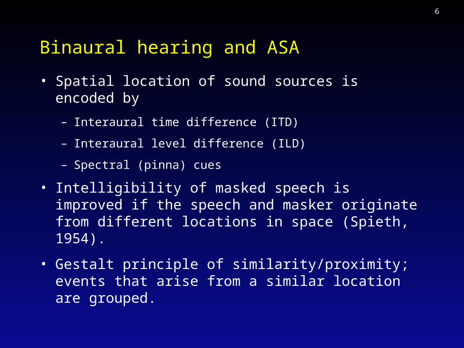
Binaural hearing and ASA
• Spatial location of sound sources is encoded by
– Interaural time difference (ITD)
– Interaural level difference (ILD)
– Spectral (pinna) cues
• Intelligibility of masked speech is improved if the speech and masker originate from different locations in space (Spieth, 1954).
• Gestalt principle of similarity/proximity; events that arise from a similar location are grouped.

7
Binaural processor for MD ASR
• Assumptions:
– Two sound sources, speech and an interfering sound;
– Sources spatialised by filtering with realistic head-related impulse responses (HRIR);
– Reverberation may be present.
• Key features of the system:
– Components of the same source identified by common azimuth;
– Azimuth estimated by ITD, with ILD constraint;
– Spectral normalisation technique for handling convolutional distortion due to HRIR filtering and reverberation.

8
Block diagram of the system
Auditoryfilterbank Envelope
Precedencemodel
Groupingcommonazimuth
Crosscorrelation
MissingdataASR
9
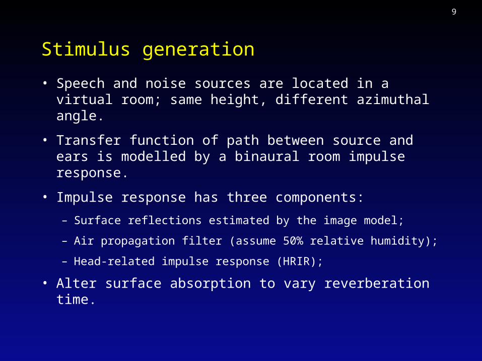
Stimulus generation
• Speech and noise sources are located in a virtual room; same height, different azimuthal angle.
• Transfer function of path between source and ears is modelled by a binaural room impulse response.
• Impulse response has three components:
– Surface reflections estimated by the image model;
– Air propagation filter (assume 50% relative humidity);
– Head-related impulse response (HRIR);
• Alter surface absorption to vary reverberation time.

10
Virtual room
Length 6mWidth 4m
Height 3mSpeechsource
Noise source

11
Auditory periphery
• Cochlear frequency analysis modelled by bank of 32 gammatone filters, rectify and cube root compress.
• Instantaneous envelope computed.
• Smooth envelope and downsample to obtain ‘rate map’; feature vectors for the recogniser.
Freq
uenc
y
Time
12
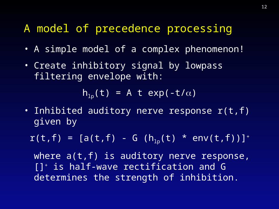
A model of precedence processing
• A simple model of a complex phenomenon!
• Create inhibitory signal by lowpass filtering envelope with:
hlp(t) = A t exp(-t/)
• Inhibited auditory nerve response r(t,f) given by
r(t,f) = [a(t,f) - G (hlp(t) * env(t,f))]+
where a(t,f) is auditory nerve response, []+ is half-wave rectification and G determines the strength of inhibition.
13
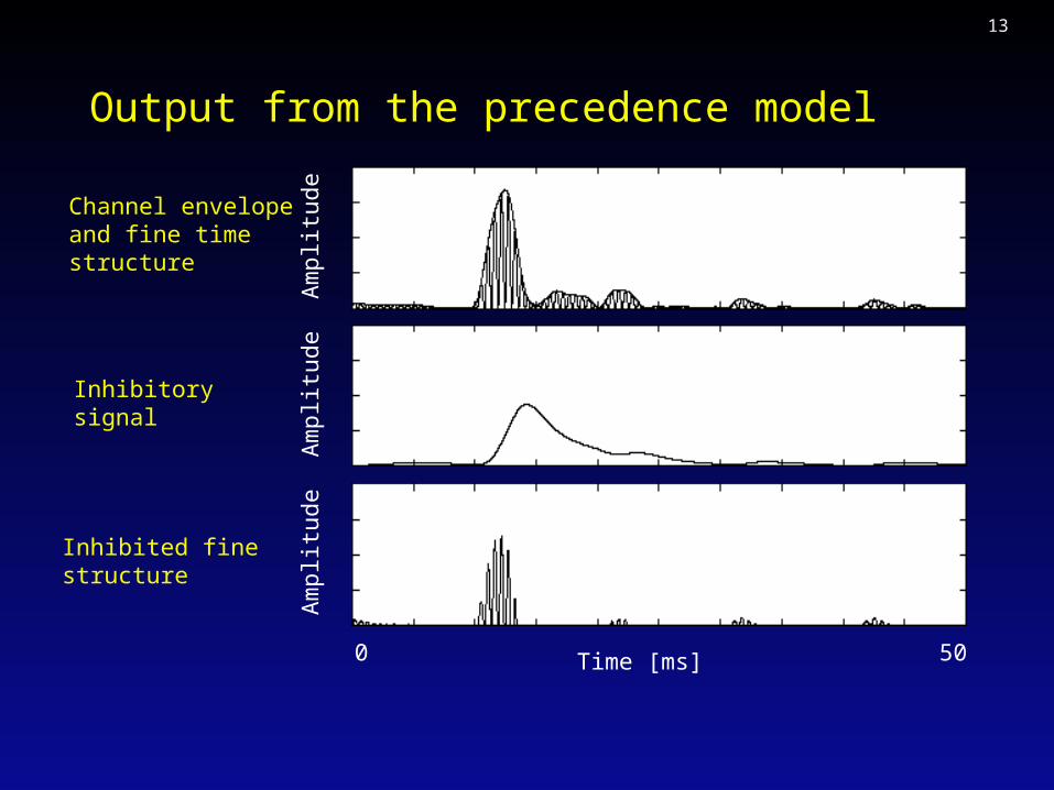
Output from the precedence model
Am
plit
ude
Am
plit
ude
Am
plit
ude
Time [ms]0 50
Channel envelopeand fine timestructure
Inhibitorysignal
Inhibited finestructure

14
Azimuth estimation
• Estimate ITD by computing cross-correlation in each frequency band.
• Form a cross-correlogram (CCG), a two-dimensional plot of ITD against frequency band.
• Sum across frequency, giving pooled cross-correlogram.
• Warp to azimuth axis, since HRIR-filtered sounds show weak frequency-dependence in ITD.
• Sharpen CCG by replacing local peaks with narrow Gaussians – skeleton CCG. Like lateral inhibition.

15
Cross-correlogram (ITD)
Interaural time difference (ITD)
Cha
nnel
cen
tre
freq
uenc
y
Mixture of maleand female speech
Azimuths:Male speech +20 degFemale speech -20 deg
16
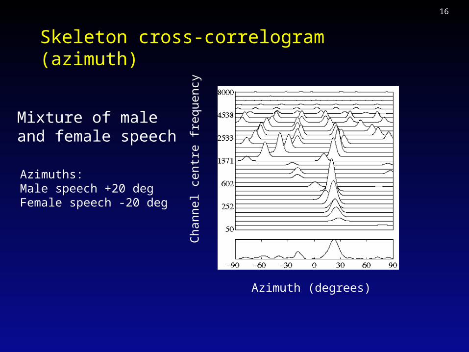
Skeleton cross-correlogram (azimuth)
Azimuth (degrees)
Cha
nnel
cen
tre
freq
uenc
y
Mixture of maleand female speech
Azimuths:Male speech +20 degFemale speech -20 deg
17
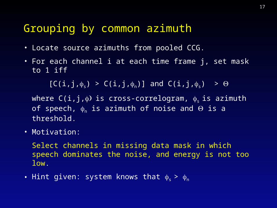
Grouping by common azimuth
• Locate source azimuths from pooled CCG.
• For each channel i at each time frame j, set mask to 1 iff
[C(i,j,s) > C(i,j,n)] and C(i,j,s) >
where C(i,j,is cross-correlogram, s is azimuth of speech, n is azimuth of noise and is a threshold.
• Motivation:
Select channels in missing data mask in which speech dominates the noise, and energy is not too low.
• Hint given: system knows that s > n

18
ILD constraint
• Compute interaural level difference as:
ILD(i,j) = 10 log10 [engR(i,j)/engL(i,j)]
where engk(i,j,n) is energy in channel i at time frame j for ear k.
• Store ‘ideal’ ILD for a particular azimuth in a lookup table.
• Cross-check observed ILD against ‘ideal’ ILD for observed azimuth; if they do not agree to within 0.5 dB set mask to zero.

19
Spectral energy normalisation
• HRIR filtering and reverberation introduces convolutional distortion.
• Usually normalise by mean and variance of features in each frequency band; but what if data is missing?
• Current approach is simple: normalise by the mean of the N largest reliable feature valuesYr in each channel.
• Motivation:
Features that have high energy and are marked as reliable should be least affected by the noise background.

20
A priori mask
• To assess limits of the missing data approach, we employ an a priori mask.
• Derived by measuring the difference between the rate map for clean speech and its noise/reverberation contaminated counterpart.
• Only set mask elements to 1 if this difference lies within a threshold value (tuned for each condition).
• Should give near-optimal performance.

21
Masks estimated by binaural grouping
Rate maps A priori mask
Mask estimated bybinaural processor
Mixture of speech (+20 deg azimuth) and interfering talker (-20 deg azimuth)SNR 0dBTop: anechoic Bottom: T60 reverberation time of 0.3 sec
22
Evaluation
• Hidden Markov model (HMM) recogniser, modified for missing data approach.
• Tested on 240 utterances from TiDigits connected digit corpus.
• 12 word-level HMMs (silence, ‘oh’, ‘zero’ and ‘1’ to ‘9’).
• Noise intrusions from Cooke’s (1993) corpus; male speaker and rock music.
• Baseline recogniser for comparison, trained on mel-frequency cepstral coefficients (MFCCs) and derivatives.

23
Example sounds
‘one five zero zero six’, male speaker, anechoic
With T60 reverberation time 0.3 sec
With interfering male speaker, 0 dB SNR, anechoic, 40 degrees azimuth separation
Two speakers, T60 reverberation time 0.3 sec

24
Effect of reverberation (anechoic)
Reverberation time 0 sec
MFCC
A priori
BinauralA
ccur
acy
[%]
Signal-to-noise ratio (dB)
Male speech masker40 degrees separation

25
Effect of reverberation (small office)
Reverberation time 0.3 sec
MFCC
A priori
BinauralA
ccur
acy
[%]
Signal-to-noise ratio (dB)
Male speech masker40 degrees separation

26
Effect of spatial separation (10 deg)
Signal-to-noise ratio (dB)
Acc
urac
y [%
]
MFCC
A priori
Binaural
Reverberation time 0.3 sec
27
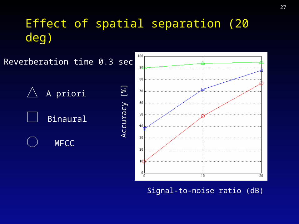
Effect of spatial separation (20 deg)
Signal-to-noise ratio (dB)
Acc
urac
y [%
]
MFCC
A priori
Binaural
Reverberation time 0.3 sec

28
Effect of spatial separation (40 deg)
Signal-to-noise ratio (dB)
Acc
urac
y [%
]
MFCC
A priori
Binaural
Reverberation time 0.3 sec

29
Effect of noise source (rock music)
Signal-to-noise ratio (dB)
Acc
urac
y [%
]
MFCC
A priori
Binaural
Reverberation time 0.3 sec

30
Effect of noise source (male speech)
Signal-to-noise ratio (dB)
Acc
urac
y [%
]
MFCC
A priori
Binaural
Reverberation time 0.3 sec
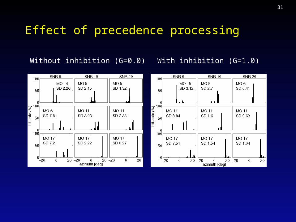
31
Effect of precedence processing
Without inhibition (G=0.0) With inhibition (G=1.0)

32
Summary of results
• The binaural missing data system is more robust than a conventional MFCC-based recogniser when interfering sounds and reverberation are present.
• The performance of the binaural system depends on the angular separation between sources.
• Source characteristics influence performance of binaural system; most helpful when spectra of speech and interfering sounds substantially overlap.
• Performance of binaural system is close to a priori masks in anechoic conditions; room for improvement elsewhere.

33
Conclusions and future work
• Combination of binaural model and missing data framework appears promising.
• However, still far from matching human performance.
• Major outstanding issues:
– Better model of precedence processing;
– Source identification (top-down constraints);
– Source selection (role of attention);
– Moving sound sources;
– More complex acoustic environments.
34
Additional Slides
35
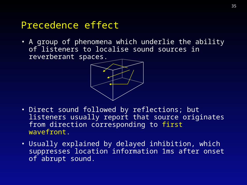
Precedence effect
• A group of phenomena which underlie the ability of listeners to localise sound sources in reverberant spaces.
• Direct sound followed by reflections; but listeners usually report that source originates from direction corresponding to first wavefront.
• Usually explained by delayed inhibition, which suppresses location information 1ms after onset of abrupt sound.
36
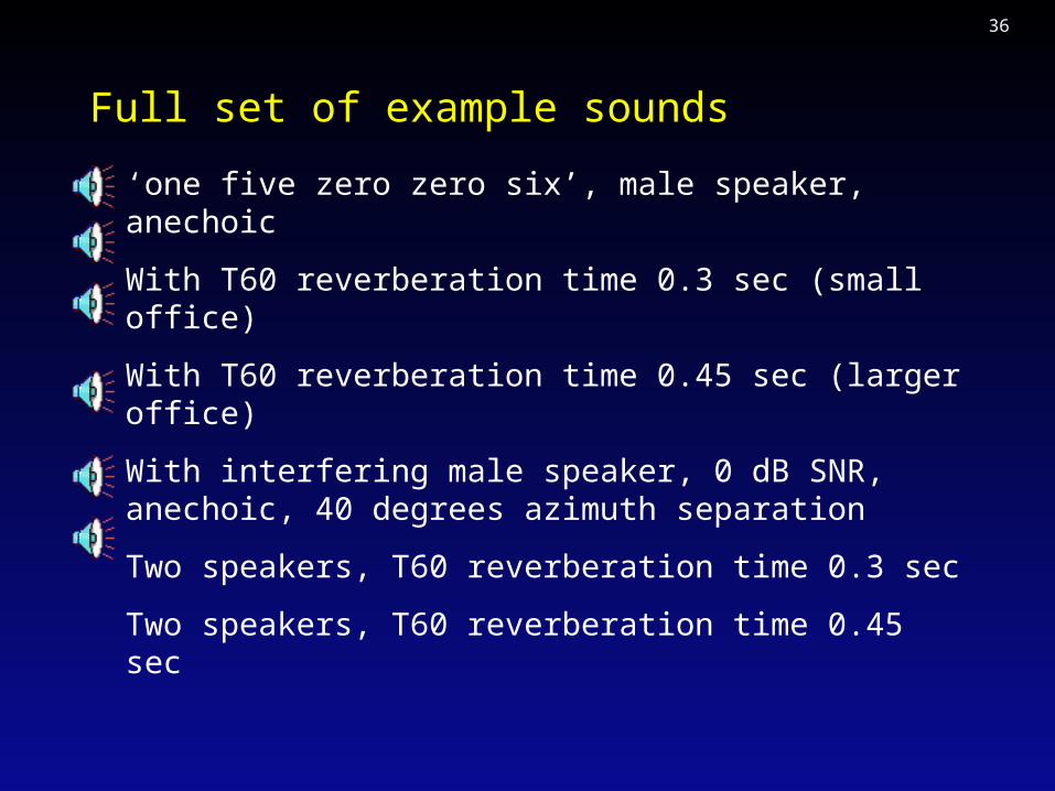
Full set of example sounds
‘one five zero zero six’, male speaker, anechoic
With T60 reverberation time 0.3 sec (small office)
With T60 reverberation time 0.45 sec (larger office)
With interfering male speaker, 0 dB SNR, anechoic, 40 degrees azimuth separation
Two speakers, T60 reverberation time 0.3 sec
Two speakers, T60 reverberation time 0.45 sec
37
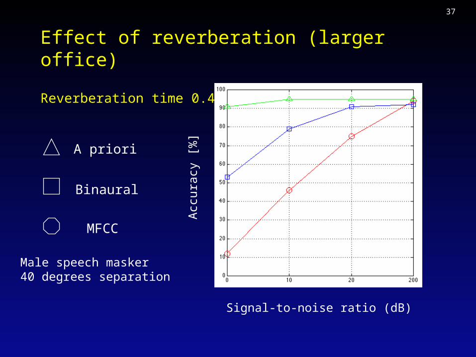
Effect of reverberation (larger office)
Reverberation time 0.45 sec
MFCC
A priori
BinauralA
ccur
acy
[%]
Signal-to-noise ratio (dB)
Male speech masker40 degrees separation

38
Effect of noise source (female speech)
Signal-to-noise ratio (dB)
Acc
urac
y [%
]
MFCC
A priori
Binaural
Reverberation time 0.3 sec