1

Limnological Analysis of the Groundwater, Biological, and Morphological Factors in Relation to Stratification and Dissolved Oxygen Levels of the North and South

Basins of Roosevelt Lake, Minnesota

Andrew Ritts Senior Integrative Exercise

March 10, 2010

Submitted in partial fulfillment of the requirements for a Bachelor of Arts degree from Carleton College, Northfield, Minnesota

2

TABLE OF CONTENTS

Abstract 3

Introduction 4

Geologic Setting 7

Methods 10

Models 11

Data 16

Discussion 29

Acknowledgements 33

References 33

Appendices 36

3

Limnological Analysis of the Groundwater, Biological, and Morphological Factors in Relation to Stratification and Dissolved Oxygen Levels of the North and South Basins of

Roosevelt Lake, Minnesota

Andrew Ritts Senior Integrative Exercise

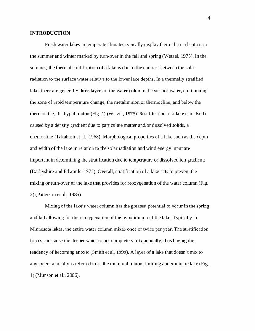
March 10, 2010 Advisors: Howard Mooers, University of Minnesota Duluth Cameron Davidson, Carleton College ABSTRACT Groundwater, biological, and morphological data were collected on Roosevelt Lake, MN, from July through August of 2009 to analyze the contrast in dissolved oxygen levels in the north and south basins of Roosevelt Lake. Chemoclines were present between 3-8 m in the north and south basins, with a second deeper chemocline present only in the north basin at depths greater than 12 m. The formation of the 3-8 m chemocline was primarily influenced by increased ionic concentrations of Ca2+, Cl-, SO4

2, Na+, Mg2+, total Fe, and total P in the groundwater between 6-9 m. Anoxic biological decomposition in the deep hypolimnion in the north basin was the principal component of the 12-15 m chemocline in the north basin. The chemoclines were related to the contrast in the dissolved oxygen levels between the north and south basins. The north basin had dissolved oxygen levels lower than about 0.1 mg/L at about 8 m that were anoxic below approximately 12 m. In contrast, the south basin had oxygen levels around 5-6 mg/L for the hypolimnion in early July that diminished throughout the summer approaching about 1-2 mg/L by late August. In coalescence with the chemoclines in the north and south basins, the crucial factors that control the dissolved oxygen level differences in the north and south basins are the morphological characteristics of the basins. The north basin’s lower fetch and sheltered surroundings result in decreased wind energy input into the north relative to the south basin. Decreased wind energy input has caused shorter time periods of destratification in the spring and fall for the north relative to the south basins, and thus reduced water column reoxygenation potential for the north basin.

Keywords: limnology, meromictic lake, thermocline, chemocline, stratification, morphology, dissolved oxygen levels

4

INTRODUCTION

Fresh water lakes in temperate climates typically display thermal stratification in

the summer and winter marked by turn-over in the fall and spring (Wetzel, 1975). In the

summer, the thermal stratification of a lake is due to the contrast between the solar

radiation to the surface water relative to the lower lake depths. In a thermally stratified

lake, there are generally three layers of the water column: the surface water, epilimnion;

the zone of rapid temperature change, the metalimnion or thermocline; and below the

thermocline, the hypolimnion (Fig. 1) (Wetzel, 1975). Stratification of a lake can also be

caused by a density gradient due to particulate matter and/or dissolved solids, a

chemocline (Takahash et al., 1968). Morphological properties of a lake such as the depth

and width of the lake in relation to the solar radiation and wind energy input are

important in determining the stratification due to temperature or dissolved ion gradients

(Darbyshire and Edwards, 1972). Overall, stratification of a lake acts to prevent the

mixing or turn-over of the lake that provides for reoxygenation of the water column (Fig.

2) (Patterson et al., 1985).

Mixing of the lake’s water column has the greatest potential to occur in the spring

and fall allowing for the reoxygenation of the hypolimnion of the lake. Typically in

Minnesota lakes, the entire water column mixes once or twice per year. The stratification

forces can cause the deeper water to not completely mix annually, thus having the

tendency of becoming anoxic (Smith et al, 1999). A layer of a lake that doesn’t mix to

any extent annually is referred to as the monimolimnion, forming a meromictic lake (Fig.

1) (Munson et al., 2006).

Epilimnion

Thermocline

Hyplimnion

Monimolimnion

Figure 1. Water column layers’ classification with (A) expressing a lake’s water column profile and (B) the corresponding classification of the lake’s layers. The density gradients are the thermocline and chemocline.The thermocline is defined by a temperature gradient, while the chemocline is defined by a particulate and dissolved solids gradient. In a meromictic lake a monimolimnion can form below a chemocline (Munson et al., 2009).

Chemocline Mixing Boundary

Mixing Boundary

Temperature Density

Dep

th

TemperatureDensity

A B

5

Epilimnion

Epilimnion

Thermocline

Hypolimnion

Hypolimnion

Summer: increasing solar radiation preferentially heats the epilimnion waters creating a heat gradient betweenthe top and bottom waters, forming a thermocline.

Thermal Stratification

Spring Turnover: After the ice melts, there are lowthermal stratification forces allowing for low wind energy inputs needed to create mixing of the water column.

Turnover Turnover

Fall Turnover: As solar energy input to the surface waters decreases, the thermocine deeens weakening thermal stratification forces.

Figure 2. Cross-Sections of cycles of water column mixing through the seasons (Munson et al., 2009).

Winter: Due to water having its greatest density at 4*C, the epilimnionwaters become cooler than the hypolimnion waters at 4*C causing inverse thermal stratification.

Summer

Winter

Spring Fall

IceInverse Themal Stratification

6

7

The purpose of this paper is to determine the cause of the lower dissolved oxygen

levels in the hypolimnion of the north basin relative to the south basin of Roosevelt Lake,

Minnesota, and, subsequently, to interpret any changes that could be made in lake

management to help control the dissolved oxygen levels of the basins. Dissolved oxygen

levels are directly related to the ability of the water column to mix and allow atmospheric

dissolution of oxygen to saturate the water column (Wetzel, 1975). In order to

characterize the mixing properties of these basins, this paper will approach the dissolved

oxygen levels in relation to the stratification characteristics of the lake through the

analysis of the groundwater, biological, and morphological components of the lake

system.

GEOLOGIC SETTING

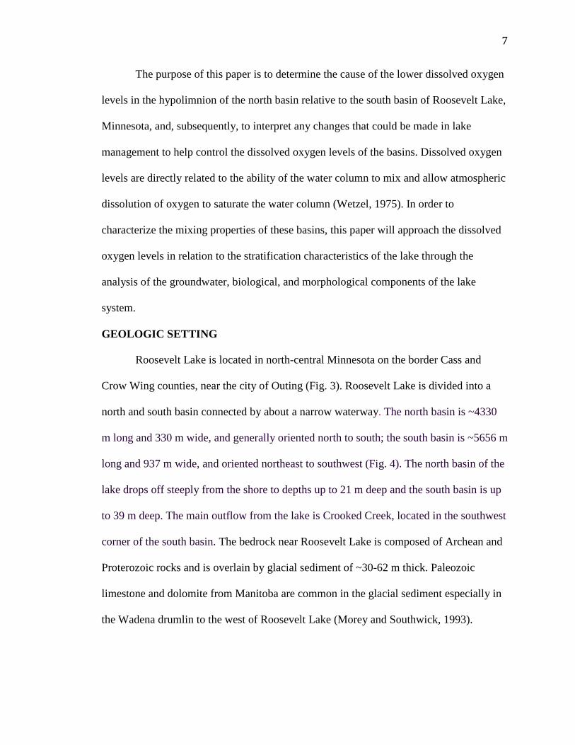
Roosevelt Lake is located in north-central Minnesota on the border Cass and

Crow Wing counties, near the city of Outing (Fig. 3). Roosevelt Lake is divided into a

north and south basin connected by about a narrow waterway. The north basin is ~4330

m long and 330 m wide, and generally oriented north to south; the south basin is ~5656 m

long and 937 m wide, and oriented northeast to southwest (Fig. 4). The north basin of the

lake drops off steeply from the shore to depths up to 21 m deep and the south basin is up

to 39 m deep. The main outflow from the lake is Crooked Creek, located in the southwest

corner of the south basin. The bedrock near Roosevelt Lake is composed of Archean and

Proterozoic rocks and is overlain by glacial sediment of ~30-62 m thick. Paleozoic

limestone and dolomite from Manitoba are common in the glacial sediment especially in

the Wadena drumlin to the west of Roosevelt Lake (Morey and Southwick, 1993).

Figure 3 . Satellite map of Roosevelt Lake, MN (A) Minnesota state wide view(B) Roosevelt Lake with sample sites (Google Earth, 2009).

B

South Basin

A

Roosevelt Lake

North Basin

8

Figure 4. Bathymetric map of (A) the north basin and (B) the south basin with the approximate location of the four sampling sites indicated with the red dots (modi�ed from MN DNR).

A

B

9

10

METHODS

YSI 350 was used to measure dissolved oxygen, temperature, and specific

conductivity at every meter of depth at four locations in Roosevelt Lake every two weeks

during July and August, 2009. Groundwater influx rates into the lake were measured at

the water depths of 0.9-1.3 m at 15 sites using a seepage meter and piezometer following

the procedures described in Rosenberry et al. (1999), and at each location GPS

coordinates and wind speed were recorded.

Darcy's flow law was applied to find the hydraulic conductivity, using the flow

rate from each seepage meter and piezometer measurements:

Q= -K*A*(H/L)

where Q is groundwater flow rate, K is the hydraulic conductivity, A is the area of

seepage, H is the difference between the height of the water in the piezometer and the

lake surface, and L is the length of the piezometer into the sediments (Fetter, 2001).

Seepage flux was corrected for water currents through using a 0.10 correction factor of

the hydraulic head:

C=(v2)/9.8, (2)

where C is the current velocity correction factor and v is the surface water velocity

current (Fetter, 2001). From Darcy’s flow law the hydraulic gradient and permeability

constants were individually averaged to allow for the calculation of the groundwater

inflow rates at deeper depths (Appendix 1). The distribution of groundwater flow into the

lake was estimated using the technique discussed in Pfannkuch and Winter (1984).

Ground water chemistry was sampled from 16 wells encompassing both the north

and south basins at depths from 6 to 27 m. Lake water was sampled with a Van Doren

11

Sampler in the epilimnion, near the top of the hypolimnion, and one meter above the lake

bottom sediments on July 13 in four different locations (Fig. 4). The Natural Resource

Institute of Duluth analyzed the lake water samples for the nutrients, P and N, and the

University of Minnesota Geoscience Laboratory determined the major cation and anion

concentrations for the groundwater and lake water samples (Appendix 2). Biological

productivity and bacterial decompositional processes of the lake were measured by

trophic status indices: secchi disk depth measurements, used to determine the depth that

solar radiation is able to penetrate; the concentration of phosphorus in the surface water,

often the limiting nutrient in plant growth; and nitrogen concentrations (Smith et al.,

1999) (Hagerthey and Kerfoot, 1998).

Morphological factors were accounted for by calculating the heat flux model

between the lake and the atmosphere using the method discussed by French et al. (2004).

The predominate wind direction was determined through field observation to be from the

northeast (Appendix 3). The heat flux model was used to estimate the time for each basin

to destratify based on different wind speeds. Ivey and Patterson’s (1984) dissolved

oxygen model was used to then estimate the time that it would take the hypolimnion of

each basin to reach full dissolved oxygen saturation levels based upon varying wind

speeds (Appendix 4).

MODELS There are four models for explaining the differences in the dissolved oxygen

levels between the north and south basins:

Groundwater

12

The differences in the dissolved oxygen levels are caused by contrasts in the net

influx rates of groundwater between the two basins. The assumption in this case is that

groundwater is anoxic throughout most depths, which was true for 12 of the groundwater

samples from below 6 m, as a result of bacterial decompositional processes listed in

Tables 1 and 2. Higher rates of groundwater influx into the hypolimnion of the north

basin would directly cause the lower oxygen levels in the north basin relative to the south

basin.

Biological

There are significant differences in dissolved oxygen levels due to contrasts in the

rates of biological productivity between the two basins (Hagerthey and Kerfoot, 1998).

Within this model the variables that are most significant in controlling the rate of algae

growth are the nutrients of phosphorus and nitrogen, while also the depth of solar

radiation within each basin’s water column. Higher rates of algal production in the north

basin would cause the depletion of dissolved oxygen levels in the lower part of the

hypolimnion for the north basin in July and August, as algal production generally peaks

during the summer (Smith et al., 1999).

Morphological

The differences in the dissolved oxygen levels in the hypolimnions in the north

and south basins are connected with the time that it takes the thermocline to destratify

and stratify the water column in the fall and spring respectively. This model is based

upon Darbyshire and Edward’s (1972) relationship of the depth of the thermocline being

positively proportional to the wind energy input divided by the heat input. The decreased

wind energy imparted into the north basin compared to the south basin would cause the

TABLE 2 . ANAEROBIC CONDITIONS: DECOMPOSITIONAL REACTIONS

Decomposition oxidation O2(g) + CH2O = CO2(g) + H2O Sul�de oxidation O2 + 1/2HS- = 1/2SO4

2- + 1/2H+ Iron oxidation 1/4O2 + Fe2++ H+ = Fe3+ + 1/2H2O Nitri�cation O2 + 1/2NH4

+ = 1/2NO3- + H+ + 1/2H2O

Manganese oxidation O2 + 2Mn2+ + 2H2O = 2MnO2(s) + 4H+ Iron sul�de oxidation 15/4O2 + FeS2(s) + 7/2H2O = Fe(OH)3(s) + 2SO4

2- + 4H+

Rection Type Reaction Formula

Rection Type Reaction Formula

TABLE 1. AEROBIC CONDITIONS: DECOMPOSITIONAL REACTIONS

Denitri�cation CH2O + 4/5NO3- = 2/5N2(g) + HCO3

- + 1/5H + 2/5H2O Manganese IV reduction: CH2O + 2MnO2(s) + 3H+ = 2Mn2+ + HCO3

-+ 2H2O Iron III reduction CH2O + 4Fe(OH)3(s) + 7H+ = 4Fe2+ +HCO3

- +10H2O Sulfate reduction CH2O + 1/2SO4

2- = 1/2HS- + HCO3- + 1/2H+

Methane fermentation CH2O + 1/2H2O = 1/2CH4(g) + 1/2HCO3- + 1/2H+

13

14

north basin to stratify earlier in the spring and destratify later in the fall, leading to

decreased time for mixing of the north basin’s water column (Fig. 5). Subsequently, there

will be lower dissolved oxygen levels in the north basin relative to the south basin

throughout the year.

Chemocline

The causes of the contrast in dissolved oxygen levels is from the presence of

dissolved ion gradients, chemoclines, within the two basins. Increases in the strength,

number, and depths of the chemoclines could be causing the lower dissolved oxygen

levels in the hypolimnion of the north basin relative to the south basin (Socolofsky and

Jirka, 2004). Similar models as above related to the stratification forces of groundwater,

biological, and morphological differences could be explanations for the causes of the

chemoclines:

Biological

The chemoclines are formed from the release of dissolved ions into the water

column from bacterial decompositional processes under reducing conditions. The types

of bacterial decompositional processes, which involve oxidation and reduction reactions,

are controlled by dissolved oxygen levels, redox conditions. Adsorption, removal of

dissolved ions from the water column, occurs under oxic conditions on the surfaces of

polyvalent ions such as oxyhydroxides of Fe, Mn, Al, and carbonates. Under hypoxic

conditions, Fe and Mn oxyhydroxides (OOH) become reduced and soluble, resulting in

the desorption of ions (Caraco and Likens, 1993).

Groundwater

Figure 5. Thermal Destratification: through the fall the stratification of the water column decreases as the thermocline gradient deepens. This allows for the turnover of the lake. The north basin (A) thermallystratifies earlier in the spring and destratifies later in the fall than the south basin (B) due to lower wind energy input into the north basin (Darbyshire and Edwards, 1972).

Legend

15

16

The formation of the chemocline was from significantly increased dissolved ions

in the groundwater with depth over the chemocline interval (Takahashi et al., 1968).

Oxidation-reduction reactions produce carbon dioxide, which can then form acidic

solutions leaching cations from the surrounding rocks, increasing the groundwater’s total

dissolved ions (Freeze and Cherry, 1979).

Morphological

The differences in the orientations and shapes of the two basins lead to contrasts

in the wind energy inputted into the two basins (Weimer and Lee, 1973). Lower wind

energy will lead to an increase in number and strength of the chemoclines as the water

column mixing potential decreases.

DATA Profile Data

July Profile Data

As shown in Figure 6, the north basin’s thermocline is generally between 3-8 m,

while the conductivity gradient representing a chemocline is between 3-8 m; the south

basin has a thermocline between 4-8 m and a chemocline between 5-8 m. There is also an

increase in conductivity shown only in the north basin with depth, forming a second

chemocline from 12-15 m. Specific conductivity is greater for all depths of the north

basin compared to the south basin, reflecting the higher total dissolved ions in the north

basin. The south basin has a fully oxygenated water column, while the north basin has

anoxic water below about 8 m (Fig. 6). The pH in the lower hypolimnion of the north and

south basins are overall not significantly different, which are slightly alkaline between

7.6-7.9.

0

5

1 0

1 5

2 0

2 5

3 0

0 3 6 9 1 2 1 52 8 02 9 03 0 03 1 03 2 03 3 03 4 03 5 03 6 03 7 0

D is s o lve d o xyg e n (m g /L )Te m p e ra tu re (*C )S p e cific C o n d u ctivty (u S )

0

5

10

15

20

25

30

0 2 4 6 8 10 12 14 16 18 20275280285290295300305310315320325

Dis s olv ed ox y gen (mg/L)Temperature (*C)Spec if ic Conduc tiv ity (uS)

0

5

10

15

20

25

0 2 4 6 8 10 12 14 16 18 20 22 24255

260

265

270

275

280

Dis s olv ed Ox y gen (mg/L)Temperature (*C)Spec if ic Conduc tiv ity (uS)

Figure 6. July profile data avarage from July 2 and July 13. (A) Upper North Basin (B) Lower North Basin (C) South Basin. Underlined are the location of the chemoclines (MN Department of Natural Resources, 2009).

Depth (m)

Depth (m)

Depth (m)

Co

nd

uctivity (u

S)

Co

nd

uctivity (u

S)

Co

nd

uctivity (u

S)

Tem

per

atu

re (°

C)

Dis

solv

ed O

xyg

en (m

g/L

)Te

mp

erat

ure

(°C

)D

isso

lved

Oxy

gen

(mg

/L)

Tem

per

atu

re (°

C)

Dis

solv

ed O

xyg

en (m

g/L

)

A

B

C

17

18

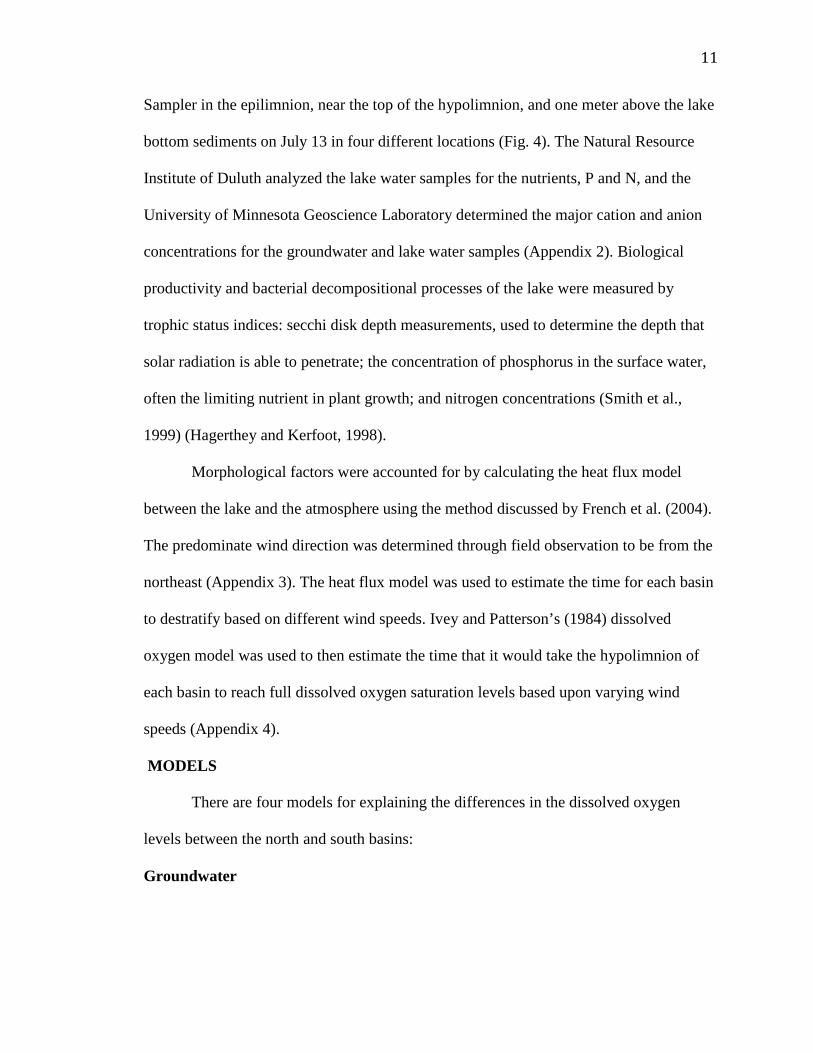
August Relative to July Profile Data

As shown in Figure 7, an important characteristic between the north and south

basins is the consistent chemocline depth relative to the changing thermocline depth. The

chemocline in the north basin remained similar, while in the south basin the gradient

increased significantly. Also, there is the pattern that the conductivity values at each level

in the water column are highest in the northern part of the north basin, and decrease

sequentially to the lowest values in the southern part of the south basin. For example, the

water at between 7-11 m, in the north basin had specific conductivity values of about 298

uS and in the south basin had values of about 272 uS.

In the north basin, there existed about a 20-25 uS/cm specific conductivity

gradient across the 3-8 m chemocline in the north compared to about a 15 uS/cm gradient

in the south basin. The north basin’s chemocline from 12-15 m is of about 15-30 uS/cm.

Now, for comparison the chemocline gradient in four meromictic lakes: Lake Mary’s

chemocline in Wisconsin is about 32 uS/cm (Weimer and Lee, 1973); Hall Lake in

Washington is about 30 uS/cm (Culver, 1977); Green Lake in New York is about 800

uS/cm; Round Lake’s in New York is about 600 uS/cm (Brunskill and Ludlam, 1969).

Groundwater Influx Rates

The total surface area of influx of the north basin was ~ 2.4E6 m2, while for the

south basin was ~1.1E7 m2; outflux surface area for the north basin was ~3.1E5 m2, and

in the south basin ~2.7E6 m2 (Fig. 8). As shown in Figure 9, the net influx rate per m2

was about three times larger in the south basin relative to the north basin at depths of 1-

1.2 m (Fig. 9). As expressed in Figure 10, the south basin would likely have a slightly

higher width ratio, however, the similarity between the width ratio and influx values

230

240

250

260

270

280

290

0

5

10

15

20

25

0 5 10 15 20 25

August Dissolved oxygen (mg/L)

August Temperature (*C)

August Specific conductivity (uS)

270

280

290

300

310

320

330

0

5

10

15

20

25

0 2 4 6 8 10 12 14 16 18 20

August Dissolved oxygen (mg/L)

August Temperature (*C)

August Specific Conductivity (uS)

Tem

pera

ture

(ºC)

Tem

pera

ture

(ºC)

Dis

solv

ed O

xyge

n (m

g/L)

Dis

solv

ed O

xyge

n (m

g/L)

Speci�c Conductivity (uS/cm)

Speci�c Conductivity (uS/cm)

Figure 7. August pro�le data averages from August 3 and August 14: (A) North Basin (B) South Basin.

A

B

19

0.0E+00

5.0E-08

1.0E-07

1.5E-07

2.0E-07

2.5E-07

3.0E-07

3.5E-07

4.0E-07

4.5E-07

Net

Influ

x (m

^3/s

/m)

North Basin South Basin

Figure 9. Groundwater net in�ux rates into the north and south basins.

North BasinSouth Basin

Lower Potential

Higher Potential

Figure 8. Groundwater flow map generated in ArcGIS. The digital elevation map, shows the approximated water table elevation contours demonstrating high to low groundwater gradients, potentials, encompassing Roosevelt Lake from the north, east, and west directions (MN DNR Data Deli, 2009). The outflow gradientpath is through the south end of the south basin.

20

North Basin

South Basin

40 80 120 161 201 241 281 322 362 402

16 33 49 65 82 98 114 130 146 163

0South Basin Distance from shore (m)

North Basin Distance from shore (m)

Distance from shore/Half width of basin

Cu

mm

ula

tive

Dis

trib

uti

on

Rat

io o

f In

flux

Figure 10. Cummulative distribution of groundwater inflow into the north and south basins as shown by south basin and north basin’s distance from the shore axis.The curves on the graphs represent varying width ratios. WR- width ratio: higher width ratios result in more uneven distribution of groundwater influx into the basin (graph modified from Pfannuch and Winter, 1984).

0

21

22

indicates that the groundwater seepage into the lake will have a similar distribution curve

across the lake bottom. This relationship illustrates that groundwater flow will be

concentrated near the shore, with approximately 80% of total groundwater flow occurring

within about 49 and 120 m from the shoreline for the north and south basins respectively

corresponding to 8-9 m and 9-12 m deep in each basin (Fig. 10) (Winter and Pfannkuch,

1984).

Chemistry

Lake

As shown in Figure 11, the anoxic 1 m above the sediments, deep hypolimnion,

water of the north basin is distinct in chemical composition from the 10 m depth, upper

hypolimnion, water of the north and south basins, and the deep hypolimnion water of the

south basin. The deep hypolimnion water of the north basin has higher concentrations of

the redox sensitive ions of Fe, Mn, P, and decreased SO42- and NO3

2- than the other layers

sampled (Hongve, 1997). The deep hypolimnion of the north basin also has higher

concentrations of Ca and Si. The north and south basins’ upper hypolimnions and south

basin’s deep hypolimnion concentrations are correspondingly similar in compositional

concentrations (Fig. 11).

Groundwater Relative to the Lake

The concentration of redox sensitive and less redox dependent ions near the

bottom of the hypolimnion in the north and south basins are less for many of the major

ions (SO42-, Fe, Cl-, Na+, Mg2+, P) compared to the groundwater at 6 and 9 m, but are

similar in alkalinity (Fig. 12). The groundwater at 9 m has higher major ion

concentrations than the groundwater at 6 m, especially in Ca2+ and Cl-. These

0

2000

4000

6000

8000

10000

12000

SO Fe K Cl Mn Na Si Mg

VSR-12

VNR-10

VSR-1m above bottom

VNR-1m above bottom

0

50

100

150

200

250

300

350

400

450

500

Ba Li P Sr F NO NO Br Al

VSR-12

VNR-10

VSR-1m above bottom

VNR-1m above bottom

Ions

Ions

Water Column Site

Water Column Site

Co

nce

ntr

atio

n (n

g/g

)C

on

cen

trat

ion

(ng

/g)

Figure 11. Lake water column chemistry comparison grouped by decreasing ion concentration: (A) Calcium is the most, (B), (C). VSR-#: south basin lake sample at depth # m; VNR-#: north basin lake sample at depth # m.

32000

37000

42000

47000

Ca

VSR-12

VNR-10

VSR-1m above bottom

VNR-1m above bottom

Ion

Co

nce

ntr

atio

n (n

g/g

)

Water Column Site

A

B

C

23

0

5

100

150

200

250

300

350

400

450

500

Ba Li P Sr F NO NO Br Al

VSR-12

VNR-10

SR-6

SR-9

0

10000

20000

30000

40000

50000

60000

70000

80000

SO Fe K Cl Mn Na Si Mg

VSR-12

VNR-10

SR-6

SR-9

Figure 12. Top of the hypolimnion chemistry relative to groundwater chemistry comparison grouped by decreasing ion concentration: (A) Calcium, (B), (C). VSR-#: south basin lake sample at depth # m; SR-#: south basin groundwater sample at depth # m; VNR-#: north basin lake sample from depth # m; NR-#: north basin groundwater sample at depth #m.

Ions

Ions

Sample Site

Sample Site

0

20000

40000

60000

80000

100000

120000

Ca

VSR-12

VNR-10

SR-6

SR-9

Ion

Sample Site

Co

nce

ntr

atio

n (n

g/g

)C

on

cen

trat

ion

(ng

/g)

Co

nce

ntr

atio

n (n

g/g

)

A

B

C

24

25

groundwater depths correspond to about the middle and bottom of the metalimnion of the

lake.

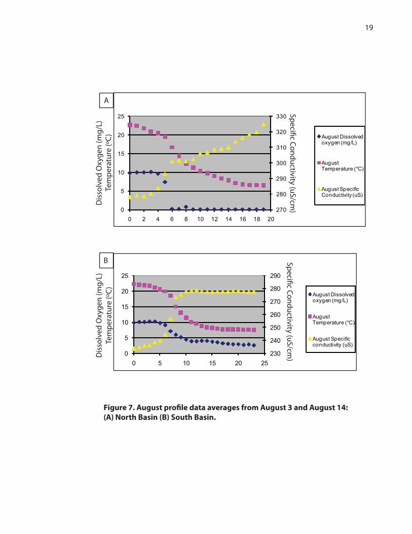
As expressed in Figure 13, the deep hypolimnion of the north basin had

significant differences in concentrations of ions, which are sensitive to redox conditions,

(Fe, Mn, P, SO42-), compared to the corresponding groundwater. The groundwater in

contrast had higher concentrations of ions that aren’t as sensitive to redox conditions as in

Ca2+, Cl-, Si, Mg2+, and Ba2+ concentrations than the corresponding lake water (Freeze

and Cherry, 1979).

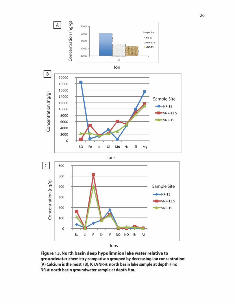
Biological

Based upon the phosphorus concentrations and secchi depth measurements the

trophic state index of the south basin increased from the high 30s to mid 40s between

July and August (Fig. 14). The trophic state index remained consistently in the low 40s

for the north basin between July and August. The trophic state indices of the north and

south basins correspond to medium productivity, which can cause anoxic water where

decompositional processes are concentrated (MN DNR). Solar energy can allow

photosynthesis to occur to depths of about 3 times secchi depth, which would be about 11

m in the north basin, and about 9-10 m in the south basin (Munson et al., 2006).

Generally, total P (TP) increases with depth shown by the significantly higher TP levels

near the sediments especially in the north basin likely from the decomposition processes

involving Fe and Mn.

Morphological

Figure 15 expresses the modeled relationship in which the south basin relative to

the north basin destratifies at a faster rate through the late summer into the fall (French,

0

2000

4000

6000

8000

10000

12000

14000

16000

18000

20000

SO Fe K Cl Mn Na Si Mg

NR-15

VNR-13.5

VNR-19

0

100

200

300

400

500

600

Ba Li P Sr F NO NO Br Al

NR-15

VNR-13.5

VNR-19

Ions

Ions

Conc

entr

atio

n (n

g/g)

Conc

entr

atio

n (n

g/g)

Figure 13. North basin deep hypolimnion lake water relative togroundwater chemistry comparison grouped by decreasing ion concentration: (A) Calcium is the most, (B), (C).VNR-#: north basin lake sample at depth # m;NR-#: north basin groundwater sample at depth # m.

Sample Site

Sample Site

30000

40000

50000

60000

70000

Ca

NR-15

VNR-13.5

VNR-19

IonC

on

cen

trat

ion

(ng

/g)

Sample Site

A

B

C

26

0.00

10.00

20.00

30.00

40.00

50.00

60.00

70.00

80.00

90.00

100.00

0.00

10.00

20.00

30.00

40.00

50.00

60.00

70.00

80.00

90.00

100.00

0

10

20

30

40

50

60

70

80

90

100

Figure 14. Biological trophic state indices, (TSI), (A) secchi disk depth (B) total P concentration (C) total N concentration.

TSI-Secchi = 60 - 14.41 ln Secchi disk (meters)TSI-P= 14.42 ln Total phosphorus (ug/L) + 4.15TSI-N = 56 + 19 ln Total nitrogen (ug/L)

A

B

C

Tro

ph

ic S

tate

Ind

exTr

op

hic

Sta

te In

dex

Tro

ph

ic S

tate

Ind

ex

North BasinSouth Basin

Legend

Epilimnion Metalimnion

Epilimnion Metalimnion

27

0

10

20

30

40

50

60

70

80

90

0 2 4 6 8 10

Wind Speed (m/s)

Day

s

Time to Destratify

Time to Reoxygenate

Figure 15. The time for the hypolimnion of the north or south basin to destratifybased upon the surface waters being 5 ºC less than the atmopheric temperature. The time for the hypolimnion or the north or south basin to reoxygenate means thetime needed for the entire water column to reach dissolved oxygen saturation levels once the basin is destratified. These are two separate processes, so the total timefor the entire water column to reach oxygen saturation levels in the fall is approximated by adding the two quantities of days together.

Sampling North Basin South Basin Date Wind Speed (m/s) Wind Speed (m/s)

July 2 2.6 3.4July 13 3.1 4.2July 24 2.5 3.2August 3 2.2 2.8August 14 2.9 4.0August 25 2.7 3.8

Legend

TABLE 3. MEASURED WIND SPEEDS

28

29

McCutcheon, and Martin, 2004). This is demonstrated by the greater magnitude of

surface heat loss in the south basin relative to the north basin for each respective wind

speed as shown in Figure 15. Figure 15 also shows the exponential relationship between

wind speed and the approximated time for the hypolimnion to attain full oxygen

saturation. Wind speeds measured on the north and south basins are shown in Table 3.

The time to for the entire water column to attain complete oxygen saturation is estimated

to be 54 days for the north basin and 39 days for the south basin, assuming that the wind

velocities for each basin respectively were 3 and 4 m/s (Ivey and Patterson, 1984).

DISCUSSION

First, an analysis of the groundwater, biological, and morphological models as

direct causes of the lower dissolved oxygen levels in the hypolimnion of the north basin

relative to the south basin. The groundwater model is not supported based upon the data

that the epilimnion’s net groundwater influx rates were determined to be about 3 times

higher into the south basin relative to the north basin, and that the groundwater influx

distribution curves into each basin were shown to be similar. The biological model is

supported to explain part of the dissolved oxygen level differences. The north basin’s

phosphorus trophic state index in the metaliminon was approximately 23 units greater

than the south basin’s index, which supports higher bacterial decompositional processes

in the hypolimnion of the north basin. The actual quantity of the phosphorus trophic state

index for the north basin corresponds to lower oxygen levels near the sediments. The

increased biological decompositional processes are not sufficient to explain the

completely, anoxic conditions below 8 m in the north basin. The morphological model

predicts differences of 1-2 month in the time for the north basin’s hypolimnion to reach

30

oxygen saturation levels compared to the south basin. The magnitude of this difference

would lead to the north basin’s hypolimnion waters to have significantly decreased

oxygen saturation levels immediately after stratification in the spring. The lower

dissolved oxygen levels in the north basin then become depleted sooner in the summer

due to biological decompositional processes.

In coalescence with the biological and morphological causes for the lower oxygen

levels in the north basin compared to the south basin, differences in the chemoclines

between the basins are also important. First, there is the direct connection between the

plummet of the oxygen levels in both the north and south basins and the 3-8 m

chemocline. The cumulative magnitude of the north basin’s chemocline from 3-8 m and

12-15 m are comparable to the chemoclines in meromictic lakes causing a layer of the

water column below a certain depth, an monimolimnion, to not turnover to any extent.

This would result in the absence of oxygenation of this monimolimnion, although, the

data in this study is not sufficient to make the degree of this statement. The difference in

the biological, morphological, and chemocline components between the north and south

basins does support a spectrum of mixing in relationship to depth that varies between the

north and south basins.

The similarity of the 3-8m chemocline in both the north and south basins can be

explained by a similar sequence in the concentration of the ions in the groundwater with

depth surrounding both basins (Fig. 16). The groundwater from the lower part of the

chemocline interval showed a significant increase in almost all ions measured. The

importance of the similarities of the concentrations of the upper part of the hypolimnions

in both the north and south basins supports that this chemocline is likely from the

Sediments

Biological: Bacterial DecompositionAnoxic desorption by sediments

Chemocline: 12-15 m

Chemocline: 3-8 m Groundwater

G1: Low dissolved solids

Tota

l Dis

solv

ed S

olid

s

Low

High

G2: High dissolved solids

Hypolimnion

Metalimnion

Ground and Lake surface levels

Epilimnion

Disso

lved O

xygen

Levels

High

Low

Wind Energy:South Basin

North Basin

Figure 16. Cross section of the north basin with outline of the lake indicated in dark blue.The contrast in groundwater composition is shown to be the cause of the chemocline from 3-8 m. The second chemocline from 12-15 m is shown to be caused by biological factors in correspondence with the lower wind energy inputted into the north basinas indicated by the smaller blue vector drawn above the lake surface.

31

32

differences in groundwater composition across this interval. The approximately 5 uS

higher magnitude of the north basin’s than the south basin’s 3-8 m chemocline is likely

from slightly increased bacterial decompositional processes occurring in the north basin.

The 12-15 m chemocline in the north basin was related to biological and

morphological factors (Fig. 16). First, the magnitude of the phosphorus and nitrogen

trophic state indices in the north basin compared to the south basin support significant

levels of bacterial decomposition near the sediments, which is in correspondence with the

12-15 m chemocline. The anaerobic decompositional processes under the low redox

conditions are responsible for the increase in dissolved solids near the sediments below

about 11 m in the north basin. There is also low correlation between groundwater and

deep hypolimnion chemistry. The morphology, due to the decreased wind energy input

into the north basins, has been conducive to allowing for the stability for the formation of

the 12-15 m chemocline. The low redux conditions have caused the increased Fe2+, Mn2+,

and Ca concentrations, leading to the desorption of the other ionic components like P and

increased Si, subsequently, causing the higher dissolved solids in the north basin.

CONCLUSION

In conclusion, these results indicate that in order to increase the dissolved oxygen

levels within the north basin’s hypolimnion, management practices such as controlling

the nutrient input from the surroundings could be significant. Also, practices involving

changing the morphology of the lake, through increasing the ability of wind energy input

could also be effective. Increasing the wind energy input into the north basin could

involve decreasing the elevation around the lake in the predominate northeast direction,

33

which holds implications for future studies of the wind energy input into the lake relative

to the surrounding topography.

ACKNOWLEDGEMENTS I would thank to thank Howard Mooers and Jason Aronson providing me with the opportunity to participate in this research project. I would also like to thank Cameron Davidson for his help in the writing process.

REFERENCES Brunskill, G. J., and Ludlam, S. D., 1969, Fayetteville-Green-Lake, New-York .1. Physical and Chemical Limnology: Limnology and Oceanography, v. 14, p. 817-829. Caraco, N. F., Cole, J. J., and Likens, G. E., 1993, Sulfate Control of Phosphorus Availability in Lakes - a Test and Reevaluation of Hasler and Einsele Model: Hydrobiologia, v. 253, p. 275-280. Computer Support Group Inc., 2009, Calculators: http://www.csgnetwork.com/h2odenscalc.html (August 2009). Culver, D. A., 1977, Biogenic Meromixis and Stability in a Soft-Water Lake: Limnology and Oceanography, v. 22, p. 667-686. Darbyshire, J., and Edwards, A., 1972, Seasonal Formation and Movement of Thermocline in Lakes: Pure and Applied Geophysics, v. 93, p. 141-149. Fetter, C.W., 2001, Applied Hydrogeology 4rth ed.: Saddle River, NJ, Prentice Hall, p. 113-140. Freeze, R.A., Cherry, J.A., 1979, Groundwater: Englewood Cliffs, NJ, Prentice Hall, p. 82-139, 237-295. French, R.H., McCutcheon, S.C., Martin, J.L., 2004, Environmental Hydraulics: McGraw-Hill, p. 5.1-6.1. EPA, Understanding Lake Ecology: http://www.epa.gov/watertrain/pdf/limnology.pdf (August 2009). Google Earth, 2009, Satellite Map Program: Google.

34

Hagerthey, S.E., Kerfoot, C.W., 1998, Groundwater Flow Influences the Biomass and Nutrient Ratios of Epibenthic Algae in a North Temperate Lake: Limnology and Oceanography, v. 43, no. 6, p.1227-1242. Hongve, D, 1997, Cycling of Iron, Manganese, and Phosphate in a Meromictic Lake: Limnology and Oceanography, v. 42., no. 4, p. 635-647. Ivey, G. N., and Patterson, J. C., 1984, A Model of the Vertical Mixing in Lake Erie in Summer: Limnology and Oceanography, v. 29, p. 553-563. MN Department of Natural Resources, 2009, Lake Finder: http://www.dnr.state.mn.us/lakefind/index.html (August 2009). MN DNR Data Deli, 2009, Digital Elevation Data: http://deli.dnr.state.mn.us (June 2009). Morey, G. B., and Southwick, D. L., 1993, Stratigraphic and Sedimentological Factors Controlling the Distribution of Epigenetic Manganese Deposits in Iron- Formation of the Emily District, Cuyuna Iron Range, East-Central Minnesota: Economic Geology and the Bulletin of the Society of Economic Geologists, v. 88, p. 104-122. Munson, B.H., Axler, R., Hagley, C., Host, G., Merrick, G., Richards, C., 2009, Monitoring Minnesota Lakes: http://WaterOntheWeb.org (November 2009). Patterson, J. C., Allanson, B. R., and Ivey, G. N., 1985, A Dissolved-Oxygen Budget Model for Lake Erie in Summer: Freshwater Biology, v. 15, p. 683-694. Pfannkuch, H. O., and Winter, T. C., 1984, Effect of Anisotropy and Groundwater System Geometry on Seepage through Lakebeds .1. Analog and Dimensional Analysis: Journal of Hydrology, v. 75, p. 213-237. Rosenberry, D.O., LaBaugh, J.W., Hunt, R.J. 2008, Field Techniques for Estimating Water Fluxes Between Surface Water and Groundwater: U.S. Geological Survey, p. 43-67. Smith, V. H., Tilman, G. D., and Nekola, J. C., 1999, Eutrophication: impacts of excess nutrient inputs on freshwater, marine, and terrestrial ecosystems: Environmental Pollution, v. 100, p. 179-196. Socolofsky, S.A., Jirka, G.H., 2004, 23 Aug. 2009, Mixing in lakes and reservoirs, p.160-200, https://ceprofs.civil.tamu.edu/kchang/ocen689/ocen689ch9.pdf.

35

Takahash. T., Broecker, W., Li, Y. H., and Thurber, D., 1968, Chemical and Isotopic Balances for a Meromictic Lake: Limnology and Oceanography, v. 13, p. 272- 279. Weimer, W. C., and Lee, G. F., 1973, Some Considerations of Chemical Limnology of Meromictic Lake Mary: Limnology and Oceanography, v. 18, p. 414-425. Wetzel, R. G., 1975, Limnology: Philadelphia, Saunders, xii, 743 p. Winter, T. C., and Pfannkuch, H. O., 1984, Effect of Anisotropy and Groundwater System Geometry on Seepage through Lakebeds .2. Numerical-Simulation Analysis: Journal of Hydrology, v. 75, p. 239-253.

south influx

current correction

factor corrected

a*h/l area*h/l area (m2) area (in.2) K (m/s) K corrected

(m/s) Q(L/s) Q (mL/min)

SP-1 0.00E+00 7.19E-03 7.19E-03 2.68E-01 4.15E+02 2.98E-06 2.98E-06 2.14E-08 1.29E+00

SP-2 0.00E+00 8.32E-02 8.32E-02 2.68E-01 4.15E+02 2.61E-07 2.61E-07 2.17E-08 1.30E+00

SP-2a 0.00E+00 8.32E-02 8.32E-02 2.68E-01 4.15E+02 6.41E-08 6.41E-08 5.33E-09 3.20E-01

SP-4 0.00E+00 4.39E-03 4.39E-03 2.68E-01 4.15E+02 4.25E-06 4.25E-06 1.87E-08 1.12E+00

SP-5 0.00E+00 7.54E-02 7.54E-02 2.68E-01 4.15E+02 5.24E-07 5.24E-07 3.96E-08 2.37E+00

SP-6 1.02E-01 3.36E-03 2.79E-03 2.68E-01 4.15E+02 1.44E-05 1.20E-05 4.02E-08 2.41E+00

SP-8 1.02E-01 2.88E-02 2.82E-02 2.68E-01 4.15E+02 8.82E-07 8.64E-07 2.49E-08 1.49E+00

Averages 3.34E-06 2.99E-06 south

outflux

SP-7 1.02E-01 -1.65E-03 -2.22E-03 2.68E-01 4.15E+02 -4.22E-06 -5.66E-06 9.37E-09 5.62E-01

SP-9 1.02E-01 -1.31E-03 -1.98E-03 2.68E-01 4.15E+02 -8.70E-06 -1.32E-05 1.72E-08 1.03E+00

Averages 6.46E-06 9.43E-06

north i nflux

SP-10 1.02E-01 9.02E-04 4.46E-04 2.68E-01 4.15E+02 1.15E-04 5.69E-05 5.13E-08 3.08E+00

SP-11 1.02E-01 4.92E-03 4.46E-03 2.68E-01 4.15E+02 8.85E-06 8.03E-06 3.95E-08 2.37E+00

SP-12 1.02E-01 2.99E-03 2.23E-03 2.68E-01 4.15E+02 1.01E-05 7.54E-06 2.25E-08 1.35E+00

SP-13 1.02E-01 2.37E-03 1.77E-03 2.68E-01 4.15E+02 2.70E-05 2.01E-05 4.76E-08 2.86E+00

SP-14 0.00E+00 1.12E-03 1.12E-03 2.68E-01 4.15E+02 3.85E-05 3.85E-05 4.30E-08 2.58E+00

Averages 3.99E-05 2.62E-05 north

outflux

SP-3 0.00E+00 -2.03E-02 -2.03E-02 2.68E-01 4.15E+02 9.26E-07 9.26E-07 -1.88E-08 1.13E+00

SP-15 1.00E-01 -5.98E-03 -5.54E-03 2.68E-01 4.15E+02 3.40E-06 3.14E-06 -1.88E-08 1.13E+00

Averages 2.16E-06 2.04E-06

Appendix 1A . SEEPAGE INPUTS FOR DARCY FLOW CALCULATION

*

*

SP-#: seepage sample site #

36

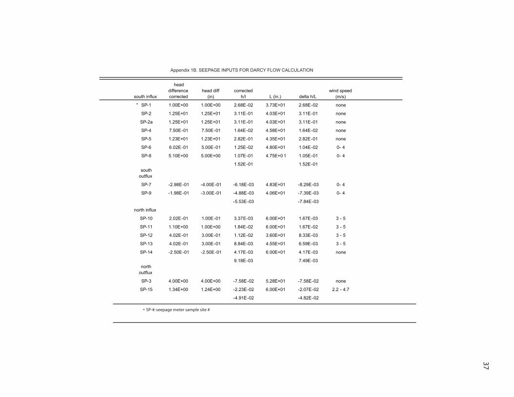
south influx

head difference corrected

head diff (in)

corrected h/l L (in.) delta h/L

wind speed (m/s)

SP-1 1.00E+00 1.00E+00 2.68E-02 3.73E+01 2.68E-02 none

SP-2 1.25E+01 1.25E+01 3.11E-01 4.03E+01 3.11E-01 none

SP-2a 1.25E+01 1.25E+01 3.11E-01 4.03E+01 3.11E-01 none

SP-4 7.50E-01 7.50E-01 1.64E-02 4.58E+01 1.64E-02 none

SP-5 1.23E+01 1.23E+01 2.82E-01 4.35E+01 2.82E-01 none

SP-6 6.02E-01 5.00E-01 1.25E-02 4.80E+01 1.04E-02 0- 4

SP-8 5.10E+00 5.00E+00 1.07E-01 4.75E+0 1 1.05E-01 0- 4

1.52E-01 1.52E-01 south

outflux

SP-7 -2.98E-01 -4.00E-01 -6.18E-03 4.83E+01 -8.29E-03 0- 4

SP-9 -1.98E-01 -3.00E-01 -4.88E-03 4.06E+01 -7.39E-03 0- 4

-5.53E-03 -7.84E-03

north influx

SP-10 2.02E-01 1.00E-01 3.37E-03 6.00E+01 1.67E-03 3 - 5

SP-11 1.10E+00 1.00E+00 1.84E-02 6.00E+01 1.67E-02 3 - 5

SP-12 4.02E-01 3.00E-01 1.12E-02 3.60E+01 8.33E-03 3 - 5

SP-13 4.02E-01 3.00E-01 8.84E-03 4.55E+01 6.59E-03 3 - 5

SP-14 -2.50E-01 -2.50E-01 4.17E-03 6.00E+01 4.17E-03 none

9.18E-03 7.49E-03 north

outflux

SP-3 4.00E+00 4.00E+00 -7.58E-02 5.28E+01 -7.58E-02 none

SP-15 1.34E+00 1.24E+00 -2.23E-02 6.00E+01 -2.07E-02 2.2 - 4.7

-4.91E-02 -4.82E-02

Appendix 1B. SEEPAGE INPUTS FOR DARCY FLOW CALCULATION

*

* SP-#: seepage meter sample site #

37

Site Dissolved Oxygen (mg/L)

Depth (m)

Al Ba Ca Fe K Li Cl Mg Mn Na

NR - 1 0 15 2.99 20.32 49755.00 294.90 1302.50 4.56 1552 14130.00 456.20 4290.00

NR - 2 0 15 0.92 48.56 58185.00 1219.00 1226.50 4.95 8235 15330.00 255.50 4725.50

NR - 3 0.73 26 6.03 33.22 57125.00 14.30 1330.00 7.35 6120 13915.00 39.43 4819.50

NR - 4 0.14 15 4.59 47.39 73770.00 221.10 1779.00 7.21 509 17285.00 607.75 5149.50

SH - 1 0 20 5.07 44.16 49085.00 4530.00 1070.00 6.02 1270 11705.00 354.05 6350.50

SH - 2 ua ua 1.23 60.83 48835.00 40.47 1743.50 3.43 589 13665.00 92.65 12960.00

SPG - 1 ua 0 10.80 39.97 61925.00 13.43 1413.00 3.34 475 16175.00 81.19 4575.50

SR - 1 0 6 11.25 43.56 49020.00 7833.00 795.65 1.66 602 9880.50 346.55 4196.50

SR - 2 0 27 8.78 89.38 57640.00 10410.00 934.90 3.05 446 9337.50 358.75 4076.00

SR - 3 0 9 30.83 85.18 96890.00 12760.00 1066.50 6.15 74326 25560.00 369.45 20965.00

SR - 4 0 18 8.59 57.35 47395.00 366.40 1640.00 5.50 943 14315.00 64.01 15355.00

SR - 5 3.33 6 153.10 9.37 25490.00 132.40 831.30 7.15 42008 6913.50 4.54 28905.00

SR - 6 0 23 1.49 41.74 17560.00 239.70 973.10 5.07 364 5796.00 90.31 2542.50

SR - 7 ua ua 3.76 56.43 50255.00 38.60 1599.00 4.23 414 13650.00 236.50 4803.00

SR - 8 ua ua 1.09 64.40 55855.00 692.60 1472.50 4.56 623 13995.00 326.95 4138.50

SR - 9 0.49 18 1.85 67.81 50395.00 388.60 1273.50 2.34 4555 11435.00 143.45 8535.50

VNR -1 0.03 10 3.62 49.66 42575.00 108.85 1490.50 3.06 2191 10915.00 573.65 4982.50

VNR -1 0 19 2.78 111.55 42820.00 2395.00 1505.50 1.81 2207 11040.00 2999.00 5036.00

VNR -2 0 13.5 4.48 162.60 46210.00 4906.50 1603.00 3.72 2296 11665.00 6146.50 5208.50

VSR -1 6.67 12 0.47 43.54 37335.00 12.73 1359.50 3.19 2360 10710.00 19.30 5351.00

VSR -1 4.66 24 1.84 51.76 37415.00 161.00 1395.00 3.89 2310 10625.00 457.40 5338.00

VSR -2 6.15 12 2.23 45.75 37645.00 26.29 1312.00 3.61 2325 10695.00 34.00 5374.00

VSR -2 5.22 20 2.30 46.81 37380.00 38.05 1344.50 2.43 2312 10695.00 106.40 5408.50

Appendix 2A . GROUNDWATER AND LAKE WATER MAJOR CATION AND ANION ANALYSIS

*NR #-north basin groundwater sample # SR #-south basin groundwater sample # VNR #-north basin lake sample # VSR #-south basin lake water sample # All Ion Concentrations in ng/g.

*

†

†§

§

#

#

**

**

38

NR-north basin groundwater sampleSR-south basin groundwater sampleVNR-north basin lake sampleVSR-south basin lake water sampleConcentrations in ng/g.

Site Dissolved Oxygen (mg/L)

Depth (m)

P Si Sr F NO2 ClO3 Br NO3 SO4 PO4

NR - 1 0 15 34.64 9148.00 70.76 193.00 2 10 5 3 16487 5

NR - 2 0 15 57.31 9249.00 70.10 135.00 2 10 5 7 33321 5

NR - 3 0.73 26 43.73 9505.50 72.03 114.00 2 10 5 3 7267 5

NR - 4 0.14 15 46.49 11410.00 95.41 203.00 2 10 5 10 5836 5

SH - 1 0 20 73.76 9431.50 88.56 118.00 2 10 5 2 11448 5

SH - 2 ua ua 51.45 6643.00 201.70 231.00 2 10 5 14 3402 5

SPG - 1 ua 0 29.41 10530.00 76.06 199.00 2 10 5 76 9088 5

SR - 1 0 6 161.25 11305.00 78.87 128.00 2 10 5 4 461 5

SR - 2 0 27 175.95 11425.00 79.06 134.00 2 10 6 9 10 5

SR - 3 0 9 157.15 12005.00 100.47 97.00 2 10 15 3 20518 5

SR - 4 0 18 24.80 6031.00 206.30 218.00 2 10 5 7 3563 5

SR - 5 3.33 6 25.05 11310.00 50.73 92.00 2 10 9 1069 8339 5

SR - 6 0 23 231.80 9835.50 49.95 48.00 2 10 5 4 10 219

SR - 7 ua ua 39.52 8897.00 100.32 145.00 2 10 5 9 4445 5

SR - 8 ua ua 30.50 9773.00 67.12 152.00 2 10 7 4 5648 5

SR - 9 0.49 18 32.08 7388.00 122.75 148.00 2 10 5 14 15211 5

VNR -1 0.03 10 37.89 7487.50 74.36 135.00 2 10 5 3 3447 5

VNR -1 0 19 397.50 8148.50 76.06 128.00 14 10 9 10 2265 5

VNR -2 0 13.5 506.70 8833.00 82.05 135.00 2 10 18 3 365 5

VSR -1 6.67 12 7.94 6034.00 73.87 127.00 2 10 5 4 3406 5

VSR -1 4.66 24 38.72 7210.50 74.54 128.00 3 10 5 96 3143 5

VSR -2 6.15 12 7.40 6427.00 74.12 131.00 2 10 5 8 3308 5

VSR -2 5.22 20 18.64 6766.00 74.40 131.00 2 10 5 51 3337 5

Appendix 2B. GROUNDWATER AND LAKE WATER MAJOR CATION AND ION DATA

*

*†

†

§

§

#

#

**

**

39

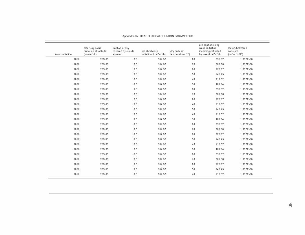
so lar rad ia tion

c lear sk y so la r rad ia tion a t la titude (kca l/m 2/h)

fraction o f sk y cove red by c louds squared

net sho rtw ave rad ia tion (kca l*m 2/h)

dry bu lb a ir tem pe rature (ºF )

a tm osphe ric long w ave rad ia tion incom ing -re flected by lake (kca l*m 2/h)

s te fan-bo ltzm an constan t (ca l*m 2/s /K 4)

1850 209 .05 0 .5 164 .57 80 338 .82 1 .357E -08

1850 209 .05 0 .5 164 .57 70 302 .88 1 .357E -08

1850 209 .05 0 .5 164 .57 60 270 .17 1 .357E -08

1850 209 .05 0 .5 164 .57 50 240 .45 1 .357E -08

1850 209 .05 0 .5 164 .57 40 213 .52 1 .357E -08

1850 209 .05 0 .5 164 .57 30 189 .14 1 .357E -08

1850 209 .05 0 .5 164 .57 80 338 .82 1 .357E -08

1850 209 .05 0 .5 164 .57 70 302 .88 1 .357E -08

1850 209 .05 0 .5 164 .57 60 270 .17 1 .357E -08

1850 209 .05 0 .5 164 .57 40 213 .52 1 .357E -08

1850 209 .05 0 .5 164 .57 50 240 .45 1 .357E -08

1850 209 .05 0 .5 164 .57 40 213 .52 1 .357E -08

1850 209 .05 0 .5 164 .57 30 189 .14 1 .357E -08

1850 209 .05 0 .5 164 .57 80 338 .82 1 .357E -08

1850 209 .05 0 .5 164 .57 70 302 .88 1 .357E -08

1850 209 .05 0 .5 164 .57 60 270 .17 1 .357E -08

1850 209 .05 0 .5 164 .57 50 240 .45 1 .357E -08

1850 209 .05 0 .5 164 .57 40 213 .52 1 .357E -08

1850 209 .05 0 .5 164 .57 30 189 .14 1 .357E -08

1850 209 .05 0 .5 164 .57 80 338 .82 1 .357E -08

1850 209 .05 0 .5 164 .57 70 302 .88 1 .357E -08

1850 209 .05 0 .5 164 .57 60 270 .17 1 .357E -08

1850 209 .05 0 .5 164 .57 50 240 .45 1 .357E -08

1850 209 .05 0 .5 164 .57 40 213 .52 1 .357E -08

Appendix 3A . HEAT FLUX CALCULATION PARAMETERS

40

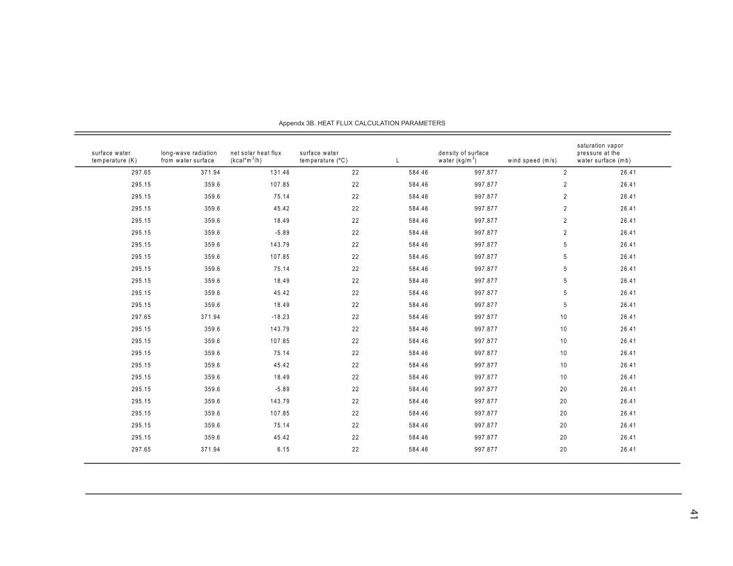
surface w ater tem pe rature (K )

long -w ave rad ia tion from w a te r su rface

net so la r hea t flux (kca l*m 2/h)

surface w ater tem pe rature (ºC ) L

density o f surface w ate r (kg /m 3) w ind speed (m /s)

sa tu ra tion vapor pressu re a t the w ate r su rface (m b)

297 .65 371 .94 131 .46 22 584 .46 997 .877 2 26.41

295 .15 359 .6 107 .85 22 584 .46 997 .877 2 26.41

295 .15 359 .6 75.14 22 584 .46 997 .877 2 26.41

295 .15 359 .6 45.42 22 584 .46 997 .877 2 26.41

295 .15 359 .6 18.49 22 584 .46 997 .877 2 26.41

295 .15 359 .6 -5 .89 22 584 .46 997 .877 2 26.41

295 .15 359 .6 143 .79 22 584 .46 997 .877 5 26.41

295 .15 359 .6 107 .85 22 584 .46 997 .877 5 26.41

295 .15 359 .6 75.14 22 584 .46 997 .877 5 26.41

295 .15 359 .6 18.49 22 584 .46 997 .877 5 26.41

295 .15 359 .6 45.42 22 584 .46 997 .877 5 26.41

295 .15 359 .6 18.49 22 584 .46 997 .877 5 26.41

297 .65 371 .94 -18 .23 22 584 .46 997 .877 10 26.41

295 .15 359 .6 143 .79 22 584 .46 997 .877 10 26.41

295 .15 359 .6 107 .85 22 584 .46 997 .877 10 26.41

295 .15 359 .6 75.14 22 584 .46 997 .877 10 26.41

295 .15 359 .6 45.42 22 584 .46 997 .877 10 26.41

295 .15 359 .6 18.49 22 584 .46 997 .877 10 26.41

295 .15 359 .6 -5 .89 22 584 .46 997 .877 20 26.41

295 .15 359 .6 143 .79 22 584 .46 997 .877 20 26.41

295 .15 359 .6 107 .85 22 584 .46 997 .877 20 26.41

295 .15 359 .6 75.14 22 584 .46 997 .877 20 26.41

295 .15 359 .6 45.42 22 584 .46 997 .877 20 26.41

297 .65 371 .94 6 .15 22 584 .46 997 .877 20 26.41

Appendx 3B. HEAT FLUX CALCULATION PARAMETERS

41

vapor pressu re o f the a tm osphere (m b)

E vapo rative heat flux (kca l/m 2/s )

E vapo rative heat flux (kca l/m 2/h )

a tm osphe ric tem pe rature (°C )

a tm osphe ric pressu re (m b)

convective heat flux (kca l/m 2/s)

convective heat flux (kca l/m 2/h)

T ota l net heat flux fo r surface w a ter o f lake (kca l/m 2/h)

34.88 -0 .03 -106.7 26.6 1020.5 -0 .0102 -36 .606 274 .76

24.99 0 .005 17.888 21.1 1020.5 0 .00199 7 .162 82.798

17.65 0 .031 110 .35 15.5 1020.5 0 .0144 51.73 -86 .942

12.27 0 .049 178 .13 10 1020.5 0 .0265 95.493 -228.2

8 .39 0 .063 227 .01 4 .4 1020.5 0 .039 140 .06 -348.58

5 .63 0 .073 261 .78 -1 .1 1020.5 0 .0511 183 .82 -451.49

34.88 -0 .07 -266.8 26.6 1020.5 -0 .0254 -91 .514 502 .06

24.99 0 .01 44.721 21.1 1020.5 0 .005 17.905 45.222

17.65 0 .08 275 .89 15.5 1020.5 0 .0359 129 .31 -330.06

12.27 0 .12 445 .32 10 1020.5 0 .0663 238 .73 -665.57

8 .39 0 .16 567 .52 4 .4 1020.5 0 .0973 350 .14 -872.23

5 .63 0 .18 654 .44 -1 .1 1020.5 0 .128 459 .56 -1095.51

34.88 -0 .15 -533.51 26.6 1020.5 -0 .0508 -183.03 698 .31

24.99 0 .02 89.442 21.1 1020.5 0 .0099 35.81 18.542

17.65 0 .15 551 .77 15.5 1020.5 0 .0718 258 .63 -702.55

12.27 0 .25 890 .65 10 1020.5 0 .133 477 .46 -1292.97

8 .39 0 .32 1135 4 .4 1020.5 0 .19 700 .28 -1789.89

5 .63 0 .36 1308.9 -1 .1 1020.5 0 .255 919 .12 -2209.51

34.88 -0 .3 -1067 26.6 1020.5 -0 .102 -366.06 1427.18

24.99 0 .05 178 .88 21.1 1020.5 0 .0199 71.62 -106.71

17.65 0 .31 1103.5 15.5 1020.5 0 .144 517 .25 -1512.95

12.27 0 .49 1781.3 10 1020.5 0 .265 954 .93 -2661.08

8 .39 0 .63 2270.1 4 .4 1020.5 0 .39 14 00.56 -3625.21

5 .63 0 .73 2617.8 -1 .1 1020.5 0 .511 1838.24 -4449.86

Appendix 3C . HEAT FLUX CAULCULATION PARAMETERS

42

43

Appendix 3D: Heat Flux Model

Heat exchange between the surface of the lake and the atmosphere was estimated

through the following model:

K= S +H

where K is net heat flux (kcal/m2/h), S is net solar heat flux, and H is heat flux form

convection.

Net solar heat flux (S) was estimated as

S=0.94(c)[1-0.65f2]+ (0.113)*[(1.16x1013)(1+0.17f2d+460)6]-

(1/0.278)[0.97(1.357x10-8)(w4)]

where c is clear sky solar radiation, f is the fraction of the sky covered by clouds, d is the

dry bulb air temperature, w is the temperature of the water surface.

Net convective heat flux (H) was estimated as:

H=[(597-0.57*w)*d*[(3x10-9)*q*(v -o))]*(6.19x10-4)*b*[(w - t)/(r - u)]

where d is density of surface water, q is the wind speed at surface, v is the saturation

vapor pressure at the water surface, o is the vapor pressure of the atmosphere, b is the

atmospheric pressure, w is the surface water temperature, t is the atmospheric

temperature, r is the saturation vapor pressure at the water surface, u is the vapor pressure

of the atmosphere (French, McCutcheon, and Martin, 2004).

w ind speed( m /s) f s (m g/m 3 ) m ph s/day day f c w

2 1 .68339E -06 12396.71 4 .74 85.23 0 .15 0 .00 0 1 .2949E -07

3 2 .61183E -06 12396.71 7 .10 54.93 0 .23 0 .00 0 2 .0091E -07

4 3 .59439E -06 12396.71 9 .47 39.92 0 .31 0 .00 0 2 .7649E -07

5 4 .6287E -06 12396.71 11.84 31.00 0 .40 0 .00 0 3 .5605E -07

6 5 .71265E -06 12396.71 14.21 25.12 0 .49 0 .00 0 4 .3943E -07

7 6 .84435E -06 12396.71 16.58 20.96 0 .59 0 .00 0 5 .2649E -07

8 8 .02213E -06 12396.71 18.94 17.89 0 .69 0 .00 0 6 .1709E -07

9 9 .24443E -06 12396.71 21.31 15.52 0 .80 0 .00 0 7 .1111E -07

10 1 .05099E -05 12396.71 23.68 13.65 0 .91 0 .00 0 8 .0845E -07

Appendix 4A . OXYGEN FLUX CALCULATION INPUTS

d v r constan t p b a

2 .06E -09 0 .000001 0 .0041 0 .069 1 .11 0 .00093 2

2 .06E -09 0 .000001 0 .0099 0 .069 1 .11 0 .00100 3

2 .06E -09 0 .000001 0 .0187 0 .069 1 .11 0 .00106 4

2 .06E -09 0 .000001 0 .0311 0 .069 1 .11 0 .00113 5

2 .06E -09 0 .000001 0 .0473 0 .069 1 .11 0 .00119 6

2 .06E -09 0 .000001 0 .0680 0 .069 1 .11 0 .00126 7

2 .06E -09 0 .000001 0 .0934 0 .069 1 .11 0 .00132 8

2 .06E -09 0 .000001 0 .1240 0 .069 1 .11 0 .00139 9

2 .06E -09 0 .000001 0 .1603 0 .069 1 .11 0 .00145 10

Appendix 4B. OXYGEN FLUX CALCULATION INPUTS

w ind speed ( m /s)

2

3

4

5

6

7

8

9

10

44

w ind speed ( m /s)

2

3

4

5

6

7

8

9

10

w ind speed ( m /s)

2

3

4

5

6

7

8

9

10

l s z y h

1000.08 12.40 13 0 .95 0 .40

1000.08 12.40 13 0 .95 0 .40

1000.08 12.40 13 0 .95 0 .40

1000.08 12.40 13 0 .95 0 .40

1000.08 12.40 13 0 .95 0 .40

1000.08 12.40 13 0 .95 0 .40

1000.08 12.40 13 0 .95 0 .40

1000.08 12.40 13 0 .95 0 .40

1000.08 12.40 13 0 .95 0 .40

x k g v

0 .0080 277 .15 0 .00092 4

0 .0080 277 .15 0 .00092 4

0 .0080 277 .15 0 .00092 4

0 .0080 277 .15 0 .00092 4

0 .0080 277 .15 0 .00092 4

0 .0080 277 .15 0 .00092 4

0 .0080 277 .15 0 .00092 4

0 .0080 277 .15 0 .00092 4

0 .0080 277 .15 0 .00092 4

Appedix 4C. OXYGEN CALULATION VARIABLES CONTINUED

Appendix 4D . OXYGEN CALULATION VARIABLES CONTINUED

45

46

Appendix 4E: Oxygen Model

Ivey and Patterson’s (1984) dissolved oxygen model for Lake Erie calculated the

oxygen flux between the atmosphere and surface of the water through the following

equation:

F=w(s-c)

where F is the flux of oxygen between the atmosphere and lake (mg O2/m2/s), w is the

gas transfer velocity (m/s), s is the dissolved oxygen saturation concentration at the water

surface (mg/L), c is the dissolved oxygen concentration of water (mg/L).

The gas transfer velocity (w) is a function positively proportional to the wind speed,

which can be modeled through the relationship (O’Connor, 1983):

w=0.114(d/v)2/3[((p*[10-3*(0.8+0.065*a)] *a2)/l)0.5/28.9]

where d is the molecular diffusivity of O2 (2.06E-9 m/s), d is the kinematic viscosity of

water (10E-6 m2/s), p is the air density, a is the wind velocity, l is the surface water

density.

The saturation concentration (s) of the water is predominately a function of water

temperature and altitude:

s=z*y*[((1-x/y)(1-gy))/(1-y)(1-g)]

where z is the equilibrium oxygen concentration at standard pressure of 1 atm, y is the

nonstandard pressure (atm), x is the partial pressure of water vapor, and

g= 0.000975-(v*1.426*10-5)+(6.436*10-8)(v2)

where v is the temperature, (°C).