1. Limits

1.1 Definition of a Limit

1.2 Computing Basic Limits

1.3 Continuity

1.4 Squeeze Theorem

1.1 Definition of a Limit

• The limit is the central object of calculus.

• It is a tool from which other fundamental definitions develop.

• The key difference between calculus and everything before is this idea.

• We say things like:a function f(x) has a limit at a point y

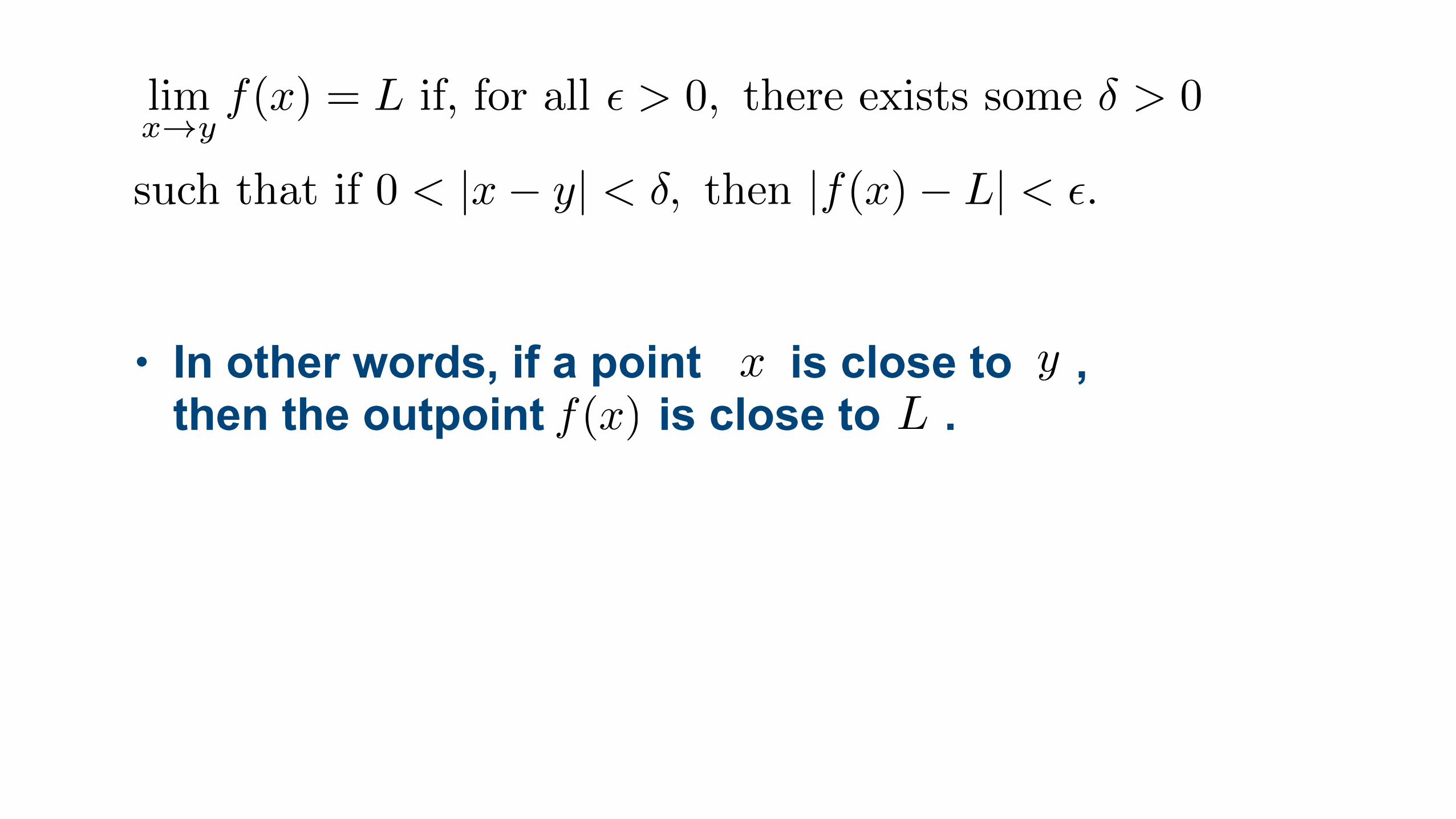
• In other words, if a point is close to , then the outpoint is close to .

yx

Lf(x)

lim

x!y

f(x) = L if, for all ✏ > 0, there exists some � > 0

such that if 0 < |x� y| < �, then |f(x)� L| < ✏.

• The limit definition does not say needs to exist!

• The special case when exists and is equal to is special, and will be discussed later.

f(x)

f(x)limy!x

f(y)

• One can sometimes visually check if a limit exists, but the definition is very important too.

• It’s a tough one the first time, but is a thing of great beauty.

1.2 Computing Basic Limits

• Computing limits can be easy or hard.

• A limit captures what the function looks like around a certain point, rather than at a certain point.

• To compute limits, you need to ignore the function’s value, and only analyze what happens nearby.

• This is what the definition attempts to characterize.

✏� �

Compute lim

x!0(x+ 1)

2

Compute lim

x!�1

x

2+ 2x+ 1

x+ 1

Compute lim

x!1

x

2+ 2x+ 1

x+ 1

Compute lim

x!0

1

x

Compute lim

x!0

px

4+ x

2

x

!

1.3 Continuity

• Sometimes, plugging into a function is the same as evaluating a limit. But not always!

• Continuity captures this property.

f is continuous at x if

limy!x

f(y) = f(x)

• Intuitively, a function that is continuous at every point can be drawn without lifting the pen.

f is continuous if it is continuous at x for all x

Discuss the continuity of f(x) =

(1x

if x 6= 0

0 if x = 0

Discuss the continuity of f(x) =

(2x+ 1 if x 1

3x

2if x > 1

• Polynomials, exponential functions, and are continuous functions.

• Rational functions are continuous except at points where the denominator is 0.

• Logarithm is continuous, because its domain is only .

sin, cos

(0,1)

1.4 Squeeze Theorem

• There are no one-size-fits-all methods for computing limits.

• One technique that is useful for certain problems is to relate one limit to another.

• A foundational technique for this is based around the Squeeze Theorem.

Suppose g(x) f(x) h(x) for some interval containing y.

) limx!y

g(x) limx!y

f(x) limx!y

h(x)

Squeeze Theorem

• We will not prove this (or any, really) theorem.

• One classic application of the theorem is computing

limx!0

sin(x)

x

• Direct substitution (which one should be very wary of when computing limits) fails.

• Indeed, plugging in yields

x = 0

sin(0)

0=

0

0= DNE

• An instructive exercise is to show that, for

cos(x) sin(x)

x

1

) lim

x!0cos(x) lim

x!0

sin(x)

x

lim

x!01

) 1 limx!0

sin(x)

x

1

) limx!0

sin(x)

x

= 1

2. Theory of the Derivative

2.1 Tangent Lines

2.2 Definition of Derivative

2.3 Rates of Change

2.4 Derivative Rules

2.5 Higher Order Derivatives

2.6 Implicit Differentiation

2.7 L’Hôpital’s Rule

2.8 Some Classic Theoretical Results

2.9 Derivatives of Inverse Functions

2.1 Tangent Lines

• Before we do any heavy lifting, let’s get a mental picture.

• One of the classical ideas behind calculus is the notion of tangent line to a function.

• This will motivate the limit definition of a derivative in the next submodule.

• A line is tangent to a function if it intersects it only once.

• This is somewhat of a simplification, in that the line is allowed to intersect multiple times outside of some small interval, but that is more advanced and theoretical than we will get into.

• Tangent lines can be constructed as limits of secant lines, i.e. lines that intersect a function in exactly two points.

• The slopes of the secant lines are computed using the classical slope formula.

• If a line passes through:

then the slope of the line is

• What is the slope of the tangent line? We need limits! This gives us the formal definition of the derivative!!!

2.2 Definition of Derivative

• The derivative is one of the two central objects in calculus.

• It measures rate of change of a function.

• In module 2, we will discuss methods for computing it, and discuss its geometric role.

• In module 3, we will use it as a tool to solve real-world problems.

• The slopes of the secant lines are computed using the classical slope formula.

• If a line passes through:

then the slope of the line is

• What is the slope of the tangent line? We need limits! This gives us the formal definition of the derivative!!!

f

0(x) = limh!0

f(x+ h)� f(x)

h

Let f(x) be a function. The derivative of f at x is

• So, the derivative is defined in terms of a limit.

• Notice that plugging in yields 0/0, so we must be careful.

• In later submodules, we will develop some nice tricks and formulae.

h = 0

Let f(x) = x. Compute f

0(x).

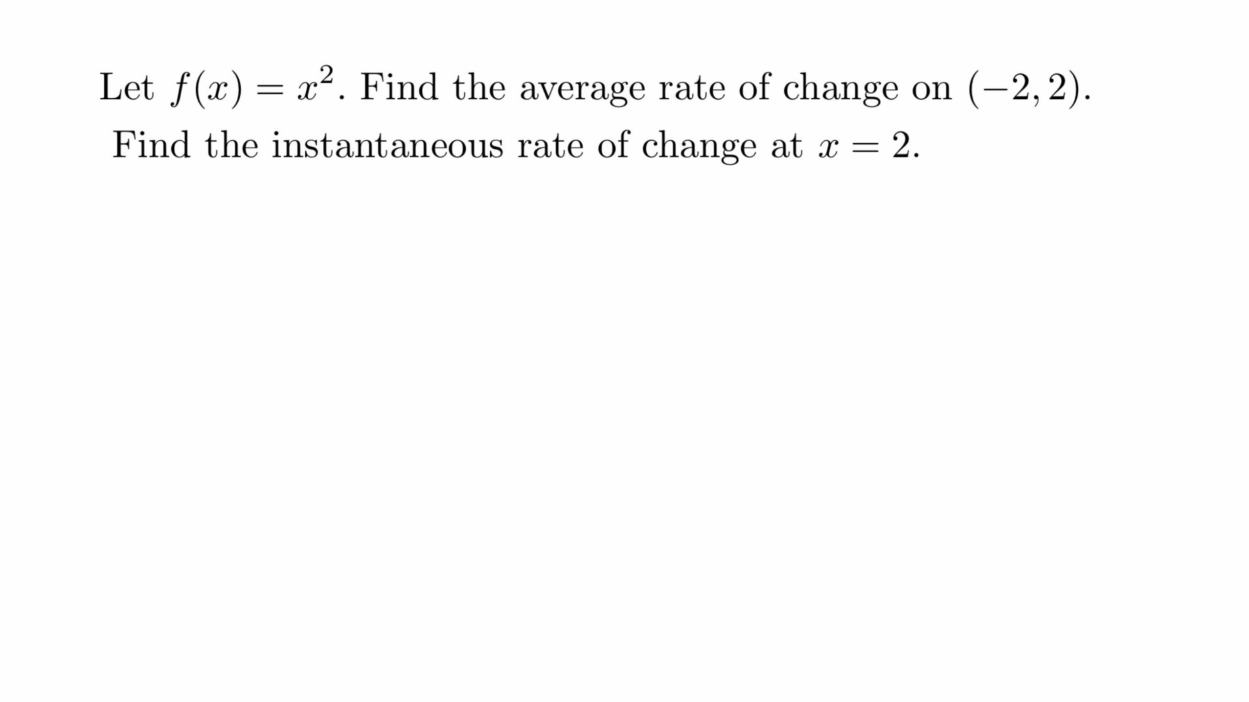
Let f(x) = x

2. Compute f

0(x).

2.3 Rates of Change

• Recall that for a general function , the slope of the secant line through may be interpreted as the average rate of change of on .

• More precisely,

• Let . Then we can say that

• This looks an awful lot like the definition of the derivative!

• Simply take the limit as

• This shrinks the interval in question to alone.

• We conclude that

• So, derivatives are equal to instantaneous rates of changes.

2.4 Derivative Rules

2.4.1 Fundamental Derivative Rules

2.4.2 Chain Rule

2.4.3 Derivatives of Exponential and Logarithmic Functions

2.4.4 Trigonometric Derivatives

2.4.5 Derivatives of Inverse Trigonometric Functions

2.4.1 Fundamental Derivative Rules

• The limit definition of the derivative is not always very convenient.

• For practical purposes, it is nice to know exactly how this definition works for certain types of functions.

• The following results are not obvious, but we will not prove them in this course.

Derivative of a Constant

[a]0 = 0

Derivative of a Polynomial

[xa]0 = ax

a�1, if a 6= 0

Let f(x) = x

4. Compute f

0(x).

Derivative of a Sum

[f(x) + g(x)]0 = f

0(x) + g

0(x)

Let f(x) = x

3 � 2x+ 1. Compute f

0(x).

Derivative of a Product

[f(x) · g(x)]0 = f

0(x) · g(x) + f(x) · g0(x)

Let f(x) = (x+ 1)

px. Compute f

0(x).

Derivative of a Quotient

f(x)

g(x)

�0=

f

0(x) · g(x)� f(x) · g0(x)g(x)2

Let f(x) =

2x� 3

x

4+ 1

. Compute f

0(x).

2.4.2 Chain Rule

• The chain rule is arguably to most foundational property of derivatives.

• It tells how to compute the derivation of a composition of functions, i.e. a function of the form f(x) = g � h(x) = g(h(x))

[g � h(x)]0 = [g0 � h(x)] · h0(x)

i.e. [g(h(x))]0 = [g0(h(x))] · h0(x)

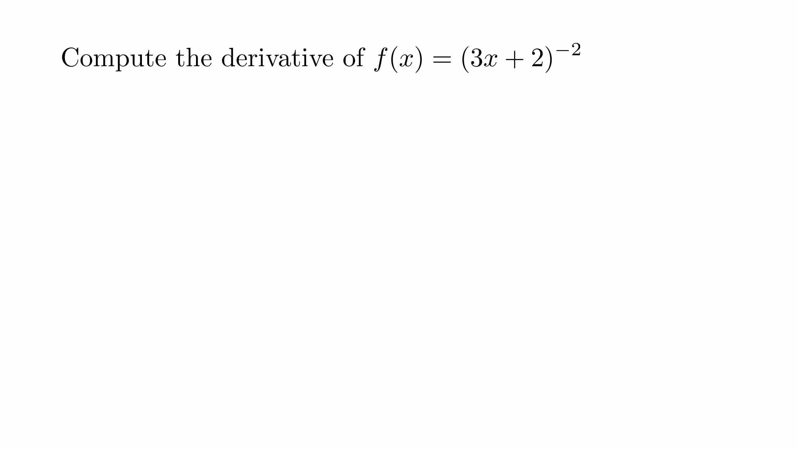
Compute the derivative of f(x) = (3x+ 2)

�2

Compute the derivative of f(x) = (x

2+ 2)

3p4x+ 1

• What if we are considering just plain old that does not appear to have the form of a composition?

• Well, we may always write:

• Taking derivatives and applying the chain rule yields:

f(x)

f(x) = f(g(x)), g(x) = x

• This emphasizes that we are always implicitly using the chain rule, even when it might appear there is no composition.

f

0(x) =f

0(g(x)) · g0(x)=f

0(x) · 1=f

0(x)

• It may be necessary to apply the chain rule iteratively:

[f(g(h(x)))]0 = f

0(g(h(x))) · g0(h(x)) · h0(x)

Compute the derivative of f(x) = (

px

2 � 1� 2)

�1

2.4.3 Derivatives of Exponential and Logarithmic Functions

• The exponential function with base is rather simple from the calculus standpoint.

• More general exponential functions have a slightly more delicate formula:

e

[ex]0 = ex

[ax]0 = ax · ln(a)

Compute

d

dx

⇥e

2x⇤

Compute

d

dz

hez

2

+ 4zi

Compute

d

dx

hxe

x

3i

• By contrast, logarithms are somewhat trickier. Derivatives of logarithms do not stay as logarithms:

[ln(x)]0 =1

x

[loga(x)]0=

1

ln(a)x

Compute

d

dx

⇥ln(x

2)

⇤

Compute

d

dy

⇥ln(y + y4)

⇤

Compute

d

dx

⇥ln(e

2x+1)

⇤

2.4.4 Trigonometric Derivatives

• The trigonometric functions all have derivatives that related to other trigonometric functions.

• The foundational ones are:

d

dx

[sin(x)] = cos(x)

d

dx

[cos(x)] = � sin(x)

Compute

d

dx

[cos(x

2+ 1)]

• We can use decompose into and then use the quotient rule to compute the derivatives of the remaining trigonometric functions.

• We will prove that

• Proving the rest of the trigonometric derivatives in a similar way is an excellent exercise.

sin(x), cos(x)

d

dx

[tan(x)] = sec(x)2

d

dx

[sec(x)] = sec(x) tan(x)

d

dx

[csc(x)] = � csc(x) cot(x)

d

dx

[cot(x)] = � csc(x)

2

Compute [tan(✓ + 1)]

0

Let f(x) = csc(x

2). Compute f

0(x).

2.4.5 Derivatives of Inverse Trigonometric Functions

• The inverse trigonometric functions also have derivatives that ought to be committed to memory for the CLEP exam.

• We will see in a later submodule how to prove these formulae starting from a general principle for derivatives of inverse functions.

• Until then, we will take the basic rules for granted.

2.5 Higher Order Derivatives

• It is possible to differentiate a function multiple times.

• The result of iterated differentiation is called a higher order derivative.

• First derivative:

• Second derivative:

• Third derivative:

• derivative: nth

f

0(x)

f

00(x)

f

(3)(x)

f

(n)(x)

Let f(x) = x

3 � 4x+ 1. Compute f

0, f

00, f

(3)

Let f(x) = e

x

2

. Compute f

0, f

00, f

(3)

Let f(x) = sin(2x). Find all values x for which f

00= 1.

Let f(x) = ln(g(x)). Compute f

00(x) in terms of g(x).

2.6 Implicit Differentiation

• All of our work has so far focused on differentiating a function where there was only one variable:

• We may at times come across an expression involving both

• In this case, is implicitly a function of .

f(x) = something depending on x

x and y

yx

• We differentiate in this case by noting that:

• This allows us to differentiate both sides of an expression, and solve for the resulting .

d

dx

[y] = y

0,

d

dx

[x] = 1.

y0

Solve for y

0: 2xy + y

2= 1

Solve for y

0:

py + 1 + x

2= y

Solve for y

0: e

xy�1= x

2

2.7 L’Hôpital’s Rule

• Recall that certain quantities are not well-defined:

• These indeterminate forms sometimes arise when taking limits of rational functions, i.e. computing limits of the form

0

0,11

limx!y

f(x)

g(x)

• In these special indeterminate cases, one can apply manipulations to in order to compute the limit.

• Another, slicker, trick is to use L’Hôpital’s rule, which we state loosely as

f(x)

g(x)

If lim

x!y

f(x) = lim

x!y

g(x) = 0 or ±1,

then lim

x!y

f(x)

g(x)

= lim

x!y

f

0(x)

g

0(x)

, provided the second limit exists.

Compute lim

x!1

x+ 1

3x� 1

Compute lim

x!0

e

x � 1

x

Compute lim

x!2

x

3 � 8

x� 2

Compute lim

x!0

sin(x)

x

Compute lim

x!0

cos(x)

x

2.8 Some Classic Theoretical Results

• This is not a course in theory, but certain results are important for the CLEP.

• Proving these would be an excellent learning experience, but is certainly not necessary. A basic understanding would suffice for the CLEP exam.

Differentiability Implies Continuity

Suppose a function f is di↵erentiable at a point x.

Then f is continuous at x.

Rolle’s Theorem

Suppose a function f is di↵erentiable on an interval (a, b).

If f(a) = f(b), then there is a point c, a < c < b such that f 0(c) = 0.

2.9 Derivatives of Inverse Functions

• We have seen already some special examples of derivatives of inverse functions: inverse trigonometric functions.

• Recall that the inverse function of is a function satisfying

Suppose f(x) = x

3+ x� 1. Compute the derivative of f

�1at x = 1.

3. Applications of the Derivative

3.1 Plotting with Derivatives

3.2 Rate of Change Problems

3.3 Some Physics Problems

3.1 Plotting with Derivatives

3.1.1 Increasing and Decreasing Functions

3.1.2 Extrema

3.1.3 Concavity

3.1.1 Increasing and Decreasing Functions

• Recall that the derivative of a function corresponds to the rate of change of a function.

• If the rate of change is positive, we say the function is increasing.

• If it is negative, we say it is decreasing.

• We can quantify this by discussing the sign of the derivative.

• Let be a function.

• If , then is increasing at .

• If , then is decreasing at .

• If , no definitive conclusion can be made without further analysis.

• Note that a function may not even be differentiable and still be increasing/decreasing.

3.1.2 Extrema

• We have seen that:

• So, what about if

• This is perhaps the most exciting aspect of differential calculus, and is a major reason it is studied by all kinds of people.

• Suppose

• Then transitions from decreasing to increasing at

• This means has a local minimum at

• Suppose

• Then transitions from increasing to decreasing at

• This means has a local maximum at

• A classic calculus problem is to find the local extrema (minima and maxima) of a function.

• To do so, set the derivative equal to 0 and check how the derivative changes sign.

• Not every place the derivative equals zero is a local extrema, however.

3.1.3 Concavity

• We saw in the previous submodule that the properties of a function being increasing, decreasing, and its local extrema are governed by its first derivative,

• A more subtle notion, concavity, is governed by the second derivative,

• A loose metaphor is in order: when plotting a function, try pouring water on it.

• If the function holds the water, it is concave up there.

• If it doesn’t hold water, it is concave down there.

• A function is concave up wherever

• A function is concave down wherever

• The second derivative can also be used to classify critical points, i.e. points where

• Second Derivative Test:

3.2 Rate of Change

• A classic application of the derivate is to compute the instantaneous rate of change of a quantity.

• Recall that the instantaneous rate of change of at is

• In contrast, the average rate of change of on the interval is

3.3 Some Physics Problems

• Another classic application of derivatives is related to the physical laws of motion.

• In this context, a one-dimensional particle’s position is given by a function

• Related quantities, like its velocity and its acceleration may be understood as certain derivatives of the position.

• Let the position of a particle be given by

• The velocity of the particle is given by

• The acceleration of the particle is given by

• So, velocity is the rate of change of position, and acceleration is the rate of change of velocity.

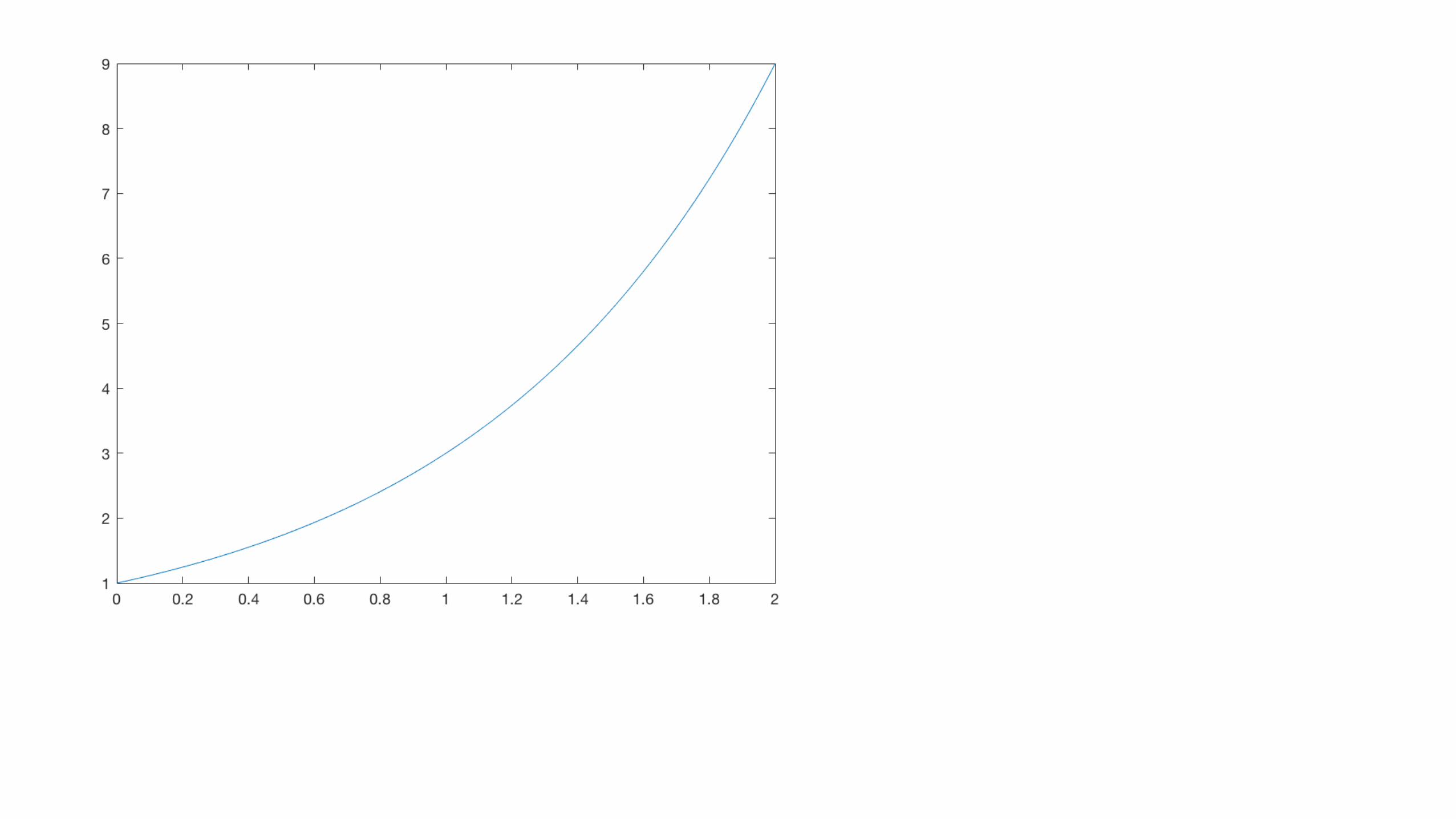
Suppose a one-dimensional particle has position p(t) = ln(t4 + t2), t > 0.

Show that the particle never changes direction.

4. Theory of the Integral

4.1 Antidifferentiation

4.2 The Definite Integral

4.3 Riemann Sums

4.4 The Fundamental Theorem of Calculus

4.5 Fundamental Integration Rules

4.6 U-Substitutions

4.1 Antidifferentiation

• We will begin our study of the integral by discussing antidifferentiation.

• As you might expect, this is the process of undoing a derivative.

Let f(x) be a function. A function F (x) is an

antiderivative of f(x) if F

0(x) = f(x).

Let f(x) = 1. Find an antiderivative of f(x).

Let f(x) = sin(x). Find an antiderivative of f(x).

Let f(x) = e

2x. Find an antiderivative of f(x).

• Notice that I am asking to find an antiderivative, not the antiderivative.

• That is because antiderivatives are not unique!

• Indeed, if is an antiderivative for , then

is also an antiderivative for any constant .

F (x)f(x)

F (x) + C

C

4.2 Definite Integral

• We will relate the antiderivative to another important object: the definite integral.

• This is a quantity that depends on two endpoint values, , and a function,

• It is written as

a, bf(x).

Z b

af(x)dx.

• The definite integral has many important interpretations.

• The most significant for us is area under the curve from to

• It is not obvious how to compute the area under the curve of a general function—this is the power of calculus!

• Let’s start with simple things.

f(x)a b.

Compute

Z 2

03dx.

Compute

Z 1

�1xdx.

Compute

Z 5

02xdx.

4.3 Riemann Sums

4.3.1 Riemman Sums Part I

4.3.2 Riemman Sums Part II

4.3.1 Riemann Sums Part I

• We have seen how to compute definite integrals of functions with certain simple properties, by exploiting well-known area formulas from geometry.

• What can we do in general? Not much yet.

• We can, however, approximate the area with Riemann sums.

• A Riemann sum approximates an integral by covering the area beneath the curve with rectangles.

• The areas of the these rectangles are more easily computed.

• This is because the width of these rectangles is fixed, and the height is given by the value of the function at a given point.

• Programmers—try coding this! It’s a classic.

Estimate

Z 4

0x

2dx with left and right Riemann sums of width 1.

4.3.2 Riemann Sums Part II

Estimate

Z 2

�1(1� x)dx with left and right Riemann sums of width 1.

4.4 The Fundamental Theorem of Calculus

• The fundamental theorem of calculus is a classic result.

• It links the derivative and the integral.

• We will not prove it, though we will use it extensively to compute areas under curves.

• Intuitively, definite integrals can be computed by evaluating an antiderivative at the endpoints of integration.

Suppose f has antiderivative F (x). Then

Z b

af(x)dx = F (b)� F (a).

Compute

Z 2

0x

2dx.

Compute

Z 2⇡

0cos(x)dx.

• When no particular endpoints are specified, the FTC suggests that we write

• Here, is an arbitrary constant.

Zf(x) = F (x) + C

C

Compute

Ze

3xdx.

Compute

Z2

x

dx.

• Another way to interpret the FTC is as stating that the derivative and integral undo each other.

• More precisely,

• This is valid for all likely to appear on the CLEP exam.

d

dx

Zf(x)dx = f(x)

f(x)

4.5 Basic Integral Rules

4.5.1 Basic Integral Rules I

4.5.2 Basic Integral Rules II

4.5.1 Basic Integral Rules I

• Using the FTC, we see that all the basic derivative rules apply, in an inverted way, to integrals.

• This means that to know the basic rules for integrals, it suffices to know the basic rules for derivatives.

For constants a, b,

Z(af(x) + bg(x))dx = a

Zf(x)dx+ b

Zg(x)dx

If n 6= �1,

Zx

ndx =

1

n+ 1x

n+1 + C

If n = �1,

Zx

ndx = ln(x) + C

Compute

Z(x

3+ 2x� 3)dx

Compute

Z(x

�1+ 1)dx

Ze

x

dx = e

x + C

Compute

Z ✓�4

x

+ 2e

x

◆dx

4.5.2 Basic Integral Rules II

Compute

Z(sin(x) + x

2)dx

Zsin(x)dx = � cos(x) + C

Zcos(x)dx = sin(x) + C

Ztan(x)dx = � ln | cos(x)|+ C

Zsec(x)dx = ln | tan(x) + sec(x)|+ C

Compute

Z(tan(✓)� cos(✓))d✓

Zdxp1� x

2= arcsin(x) + C

Zdx

1 + x

2= arctan(x) + C

Zdx

|x|px

2 � 1= sec�1(x) + C

Compute

Z �3dxp4� 4x

2

Compute

Zdy

2|y|py2 � 1

4.6 U-Substitutions

• There are many more sophisticated types of integration methods.

• These include those based on the product rule (integration by parts), special properties of trigonometric functions (trig. substitutions), and those based on tedious algebra (partial fraction decomposition).

• We focus on a method based on the chain rule.

• Recall that to compute the derivative of a composition of functions, we use the chain rule:

• According to the FTC,

• Hence,

d

dx

f(g(x)) = f

0(g(x)) · g0(x).

Zf

0(g(x))g0(x)dx = f(g(x)) + C

Zd

dx

f(g(x)) = f(g(x)) + C.

Compute

Zxe

x

2

dx

Compute

Zcos(4x+ 1)dx

Compute

Zx

3p

x

4+ 1dx

Compute

Ztan(x)dx

5. Applications of the Integral

5.1 Area Under Curves

5.2 Average Value

5.3 Growth and Decay Models

5.4 Return to Physics Problems

5.1 Area Under Curves

5.1.1 Area Under Curves Part I

5.1.2 Area Under Curves Part II

5.1.1 Area Under Curves Part I

• One of the classic applications of the integral is to compute areas.

• We defined the integral to be the area under the curve:

Z b

af(x)dx = area under f from a to b

Compute the area between x

2and the x-axis from x = 0 to x = 4.

• By convention, areas are positive. So if is negative on

• Geometry also informs the following result:

f(x) [a, b],

�Z b

af(x)dx = area under f from a to b

Z b

af(x)dx =

Z c

af(x)dx+

Z b

cf(x)dx, if a < c < b.

5.1.2 Area Under Curves Part II

• One can also compute the area between two curves with the integral.

• Suppose

• The area between on is

f(x) � g(x) on [a, b].

f(x), g(x)[a, b]

Z b

a(f(x)� g(x))dx.

Compute the area between f(x) = sin(x) and g(x) = cos(x) on

h0,

⇡

4

i.

Compute the area between f(x) = sin(x) and g(x) = cos(x) on

h0,

⇡

2

i.

Compute the area between f(x) = x and g(x) = x

2on [0, 1] .

5.2 Average Value

• The integral also has an interpretation as the average of a function’s value over an interval.

• This makes sense if you recall that an integral is approximated by Riemann sums, which are just rectangles whose heights are the function’s values.

• The following statement is also worth considering for constant functions, which clearly have constant average.

Z b

af(x)dx

• The average value of on the interval is

• So, we compute the integral, then divide by the length of the interval.

• Interpreting the integral as a sum, this bears resemblance to how the average of a finite set of numbers is computed.

f(x) [a, b]

1

b� a

Z b

af(x)dx

Compute the average value of ln(x) on [1, 100].

Compute the average value of

1

x

2+ 1

on [�1, 1].

5.3 Growth and Decay Models

• The integral allows us to solve certain basic differential equations.

• Differential equations is a huge world of mathematics, and a subject with many problems without solutions.

• It is a field of active research, including with computers.

• We will focus on an simple differential equation on the CLEP exam.

• Consider the equation in terms of the unknown function

• To solve for we do some algebra and recall the chain rule and formula for the derivative of

y(x) :

y0 = ky, some constant k.

y(x),

ln(x).

y

0 = ky

, y

0

y

= k

,Z

y

0

y

dx =

Zkdx

, ln(y) = kx+ C

, y(x) = Ce

kx

• If we have exponential growth.

• If we have exponential decay.

• The constant is determined based on details in the problem, noting that

k > 0,

k < 0,

C > 0

y(0) = C.

Suppose y0 = 2y, y(0) = 100. Find y(5).

Suppose y

0= �5y, y(0) = 1000. Find x such that y(x) = 1.

5.4 Return to Physics

• Just as we used derivatives to understand position, velocity, and acceleration of a one-dimensional particle, so too can we use integrals.

• We simply follow the fundamental theory of calculus:Z b

af

0(x)dx = f(b)� f(a).

• Let be the instantaneous velocity of a particle at time

• The position of the particle at time is and satisfies

v(t)t.

t p(t)

p0(t) =v(t)

)Z b

ap0(t)dt =

Z b

av(t)dt

) p(b) =p(a) +

Z b

av(t)dt.

Suppose a particle has instantaneous velocity v(t) = �t2

and initial position p(0) = 10. Find p(5).

• A similar game can be played with acceleration:

• With this formula for velocity, we can keep going and get a formula for position.

v0(t) = a(t)

)Z t1

t0

v0(t)dt =

Z t1

t0

a(t)dt

) v(t1) = v(t0) +

Z t1

t0

a(t)dt.

Suppose a particle has instantaneous acceleration a(t) = �10,

initial position p(0) = 0, and initial velocity v(0) = 0. Find p(5).