1

Lecture4

MGMT 650Network Models – Shortest Path

Project SchedulingForecasting

2

Shortest Path ProblemShortest Path Problem

Belongs to class of problems typically known as network flow models

What is the “best way” to traverse a network to get from one point to another as cheaply as possible?

Network consists of nodes and arcs For example, consider a transportation network

Nodes represent cities Arcs represent travel distances between cities

Criterion to be minimized in the shortest path problem not limited to distance

Other criteria include time and cost

3

Example: Shortest RouteExample: Shortest Route Find the Shortest Route From Node 1 to All

Other Nodes in the Network:

66664444

44

77

33

55 11

88

66

22

55

33

66

22

33331111

2222 5555

7777

4

Management Scientist InputManagement Scientist Input

5

Example Solution SummaryExample Solution Summary Node Minimum Distance Shortest Route

2 4 1-2 3 6 1-4-3 4 5 1-4 5 8 1-4-3-5 6 11 1-4-3-5-6 7 13 1-4-3-5-6-7

6

ApplicationsApplications

Stand alone applications Emergency vehicle routing Urban traffic planning Telecommunications

Sub-problems in more complex settings Allocating inspection effort in a production line Scheduling operations Optimal equipment replacement policies Personnel planning problem

7

Optimal Equipment Replacement Optimal Equipment Replacement PolicyPolicy

The Erie County Medical Center allocates a portion of its budget to purchase newer and more advanced x-ray machines at the beginning of each year.

As machines age, they break down more frequently and maintenance costs tend to increase.

Furthermore salvage values decrease.

Determine the optimal replacement policy for ECMC that minimizes the total cost of buying, selling and operating the machine over a

planning horizon of 5 years, such that at least one x-ray machine must be in service at all times.

Year Purchase Cost (`000)

1 170

2 190

3 210

4 250

5 300

Age Maintenance cost (`000)

Salvage value (`000)

1 50 20

2 97 15

3 182 10

4 380 0

8

Project SchedulingChapter 10

Lecture4

9

Project ManagementProject Management How is it different?

Limited time frame Narrow focus, specific objectives

Why is it used? Special needs Pressures for new or improves products or

services Definition of a project

Unique, one-time sequence of activities designed to accomplish a specific set of objectives in a limited time frame

10

Project Scheduling: PERT/CPMProject Scheduling: PERT/CPM

Project Scheduling with Known Activity Times Project Scheduling with Uncertain Activity

Times

11

PERT/CPMPERT/CPM PERT

Program Evaluation and Review Technique CPM

Critical Path Method PERT and CPM have been used to plan,

schedule, and control a wide variety of projects: R&D of new products and processes Construction of buildings and highways Maintenance of large and complex equipment Design and installation of new systems

12

PERT/CPMPERT/CPM

PERT/CPM is used to plan the scheduling of individual activities that make up a project.

Projects may have as many as several thousand activities.

A complicating factor in carrying out the activities is that some activities depend on the completion of other activities before they can be started.

13

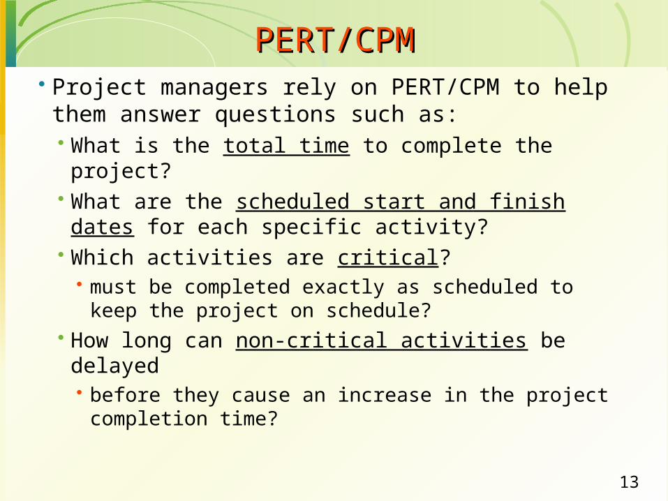
PERT/CPMPERT/CPM Project managers rely on PERT/CPM to help them

answer questions such as: What is the total time to complete the project? What are the scheduled start and finish dates for each

specific activity? Which activities are critical?

must be completed exactly as scheduled to keep the project on schedule?

How long can non-critical activities be delayed before they cause an increase in the project completion

time?

14

Project NetworkProject Network

Project network constructed to model the precedence of the

activities. Nodes represent activities Arcs represent precedence relationships of the

activities Critical path for the network

a path consisting of activities with zero slack

15

Planning and SchedulingPlanning and Scheduling

Locate new facilities

Interview staff

Hire and train staff

Select and order furniture

Remodel and install phones

Furniture setup

Move in/startup

Activity 0 2 4 6 8 10 12 14 16 18 20

16

Project Network – An ExampleProject Network – An Example

A

B

C

E

F

Locatefacilities

Orderfurniture

Furnituresetup

Interview

RemodelMove in

D

Hire andtrain

GS

8 weeks

6 weeks

3 weeks

4 weeks9 weeks

11 weeks

1 week

17

Management Scientist SolutionManagement Scientist Solution

Path Length (weeks)

Slack

A-B-F-G A-E-G C-D-G

18 20 14

2 0 6

Critical PathCritical Path

18

Three-time estimate approach the time to complete an activity assumed to

follow a Beta distribution An activity’s mean completion time is:

t = (a + 4m + b)/6 a = the optimistic completion time estimate b = the pessimistic completion time estimate m = the most likely completion time estimate

An activity’s An activity’s completion time variancecompletion time variance is is 22 = (( = ((bb--aa)/6))/6)22

Uncertain Activity TimesUncertain Activity Times

19

Uncertain Activity TimesUncertain Activity Times

In the three-time estimate approach, the critical path is determined as if the mean times for the activities were fixed times.

The overall project completion time is assumed to have a normal distribution with mean equal to the sum of the means along the

critical path, and variance equal to the sum of the variances along the

critical path.

20

ActivityImmediate

PredecessorOptimisticTime (a)

Most LikelyTime (m)

PessimisticTime (b)

A -- 4 6 8

B -- 1 4.5 5

C A 3 3 3

D A 4 5 6

E A 0.5 1 1.5

F B,C 3 4 5

G B,C 1 1.5 5

H E,F 5 6 7

I E,F 2 5 8

J D,H 2.5 2.75 4.5

K G,I 3 5 7

ExampleExample

21

Management Scientist SolutionManagement Scientist Solution

22

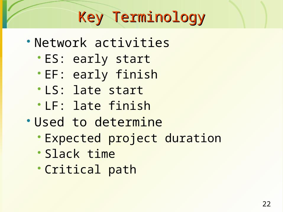
Network activities ES: early start EF: early finish LS: late start LF: late finish

Used to determine Expected project duration Slack time Critical path

Key TerminologyKey Terminology

23

Immediate Immediate CompletionCompletion

ActivityActivity DescriptionDescription PredecessorsPredecessors Time (wks)Time (wks) A Overhaul machine I ---A Overhaul machine I --- 7 7 B Adjust machine I B Adjust machine I A A 3 3 C C Overhaul machine II ---Overhaul machine II --- 6 6

D Adjust machine IID Adjust machine II C C 3 3 E Test systemE Test system B,D B,D 2 2

Example: Two Machine Example: Two Machine Maintenance ProjectMaintenance Project

Start

A 0

7

7 0

7C 0

6

6 1

7

B 7

10

3 7

10D 6

9

3 7

10

E 10

12

2 10

12

24

Normal Costs and Crash Costs

Activity

Normal Time

Normal Cost ($)

Crash Time

Crash Cost ($)

Maximum Reduction

in TimeCrash Cost per

day ($)

A Overhaul Machine I 7 500 4 800 3(800-500)/3

= 100

B Adjust machine I 3 200 2 350 1 150

C Overhaul Machine II 6 500 4 900 2 200

D Adjust machine II 3 200 1 500 2 150

E Test System 2 300 1 550 1 250

25

Linear Program for Minimum-Cost Linear Program for Minimum-Cost CrashingCrashing

Let: Let: XXii = earliest finish time for activity = earliest finish time for activity ii YYii = the amount of time activity = the amount of time activity ii is crashed is crashed

10 variables, 12 constraints

Crash activity A by 2 days

Crash activity D by 1 day

Crash cost = 200 + 150 = $350

Crash activity A by 1 day

Crash activity E by 1 day

Crash cost = 100 + 250 = $350

26

Lecture4

ForecastingChapter 16

27

Forecasting - TopicsForecasting - Topics

Quantitative Approaches to Forecasting

The Components of a Time Series

Measures of Forecast Accuracy

Using Smoothing Methods in Forecasting

Using Trend Projection in Forecasting

28

Time Series ForecastsTime Series Forecasts

Trend - long-term movement in data Seasonality - short-term regular variations in

data Cycle – wavelike variations of more than one

year’s duration Irregular variations - caused by unusual

circumstances

29

Forecast VariationsForecast Variations

Trend

Irregularvariation

Seasonal variations

908988

Cycles

30

Smoothing/Averaging MethodsSmoothing/Averaging Methods

Used in cases in which the time series is fairly stable and has no significant trend, seasonal, or cyclical effects

Purpose of averaging - to smooth out the irregular components of the time series.

Four common smoothing/averaging methods are: Moving averages Weighted moving averages Exponential smoothing

31

Sales of gasoline for the past 12 weeks at your Sales of gasoline for the past 12 weeks at your local Chevron (in ‘000 gallons). If the dealer local Chevron (in ‘000 gallons). If the dealer uses a 3-period moving average to forecast uses a 3-period moving average to forecast sales, what is the forecast for Week 13?sales, what is the forecast for Week 13?

Example of Moving Average

Past Sales

WeekWeek SalesSales WeekWeek SalesSales 1 17 7 201 17 7 20 2 21 8 182 21 8 18 3 19 9 223 19 9 22 4 23 10 204 23 10 20 5 18 11 155 18 11 15

6 166 16 12 12 22 22

32

Management Scientist SolutionsManagement Scientist Solutions

MA(3) for period 4

= (17+21+19)/3 = 19

Forecast error for period 3 = Actual – Forecast = 23 – 19

= 4

33

MA(5) versus MA(3)MA(5) versus MA(3)

Week Actual MA(3) MA(5)1 172 213 194 23 195 18 216 16 20 19.67 20 19 19.48 18 18 19.29 22 18 19

10 20 20 18.811 15 20 19.212 22 19 19

MA Forecast Graph

0

5

10

15

20

25

1 2 3 4 5 6 7 8 9 10 11 12

Week

Actu

al/M

A Fo

reca

st s

ale

valu

es

Actual

MA(3)

MA(5)

34

Exponential SmoothingExponential Smoothing

• Premise - The most recent observations might have the highest predictive value. Therefore, we should give more weight to the more recent time periods

when forecasting.

Ft+1 = Ft + (At - Ft), Formula 16.3

10

35

Linear Trend EquationLinear Trend Equation

Ft = Forecast for period t t = Specified number of time periods a = Value of Ft at t = 0 b = Slope of the line

Ft = a + bt

0 1 2 3 4 5 t

Ft

a

Suitable for time series data that exhibit a long term linear trend

36

Linear Trend ExampleLinear Trend Example

F11 = 20.4 + 1.1(11) = 32.5

Linear trend equation

Sale increases every time period @ 1.1 units

37

Actual vs ForecastActual vs Forecast

Linear Trend Example

0

5

10

15

20

25

30

35

1 2 3 4 5 6 7 8 9 10

Week

Act

ual

/Fo

reca

sted

sal

es

Actual

Forecast

F(t) = 20.4 + 1.1t

38

Measure of Forecast AccuracyMeasure of Forecast Accuracy MSE = Mean Squared Error

Week # Actual (A) Forecast(F) Error =E =A-F E(squared)1 21.6 21.5 0.1 0.012 22.9 22.6 0.3 0.093 25.5 23.7 1.8 3.244 21.9 24.8 -2.9 8.415 23.9 25.9 -2 46 27.5 27 0.5 0.257 31.5 28.1 3.4 11.568 29.7 29.2 0.5 0.259 28.6 30.3 -1.7 2.89

10 31.4 31.4 0 0

Sum of E(squared) 30.7

MSE= 3.07

39

Forecasting with Trends and Seasonal Forecasting with Trends and Seasonal Components – An ExampleComponents – An Example

Business at Terry's Tie Shop can be viewed as falling into three distinct seasons: (1) Christmas (November-December); (2) Father's Day (late May - mid-June); and (3) all other times.

Average weekly sales ($) during each of the three seasonsduring the past four years are known and given below.

Determine a forecast for the average weekly sales in year 5 for each of the three seasons.

Year Season 1 2 3 4 1 1856 1995 2241 2280 2 2012 2168 2306 2408 3 985 1072 1105 1120

40

Management Scientist SolutionsManagement Scientist Solutions

41

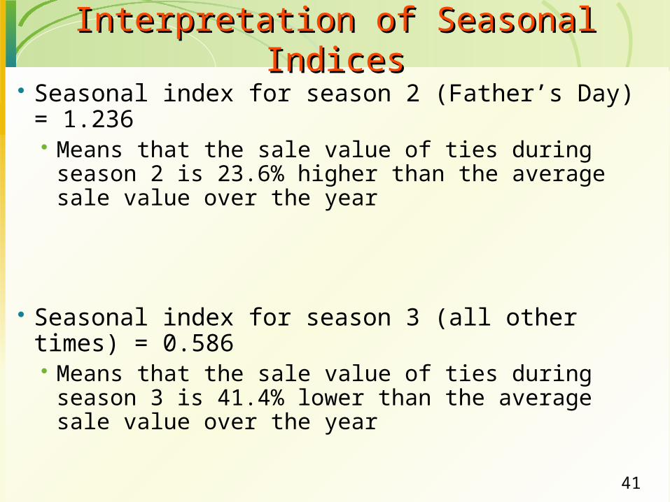
Interpretation of Seasonal IndicesInterpretation of Seasonal Indices Seasonal index for season 2 (Father’s Day) = 1.236

Means that the sale value of ties during season 2 is 23.6% higher than the average sale value over the year

Seasonal index for season 3 (all other times) = 0.586 Means that the sale value of ties during season 3 is 41.4%

lower than the average sale value over the year