1

Lecture 4

2

Random Variables (Discrete)

Real-valued functions defined on a sample space are random vars. determined by outcome of experiment, we can assign probability to possible values of it (them).

Exs: Toss 3 fair coins, let Y be number of H appearing, then Y is a random var. with possible values (0,1,2,3) with probability

P{y = 0} = P(T, T, T) = 1/8

P(y = 1) = P(T, T, H), (T, H,T), (H, T, T) = 3/8

P(y = 2) = P(T, H, H), (H, T, H), (H, H, T) = 3/8

P(y = 3) = P(H, H, H) = 1/8

Since y is between 0 and 3,

3

0

3

0

)(}){(1

i i

iyPiyP

3

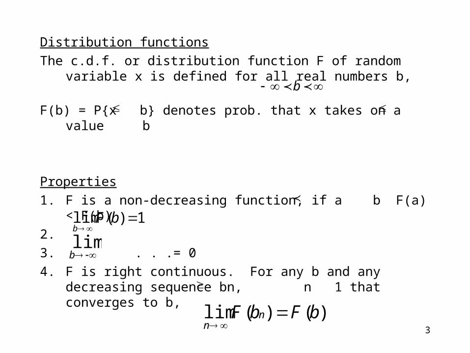
Distribution functions

The c.d.f. or distribution function F of random variable x is defined for all real numbers b,

F(b) = P{x b} denotes prob. that x takes on a value b

Properties

1. F is a non-decreasing function, if a b F(a) < F(b)

2.

3. . . .= 0

4. F is right continuous. For any b and any decreasing sequence bn, n 1 that converges to b,

b

1)(lim

bFb

blim

)()(lim bFbF nn

4

Exs: Distribution function of a random variable x is given

0 x 0

x/2 0 x 1

F(x) = 2/3 1 x 2

11/12 2 x 3

1 3 x

Calculate P{x 3}

1211)13(lim}13{lim nFnxP

nn

5

Calculate P{x = 1}

Calculate P{x ½}

Calculate P(2 x 4)

(draw graph)

61

21

32)

11(lim)1()1()1( n

FFxPxP

43)2

1(1}21{1}2

1{ FxPxP

121)2()4()42( FFxP

6

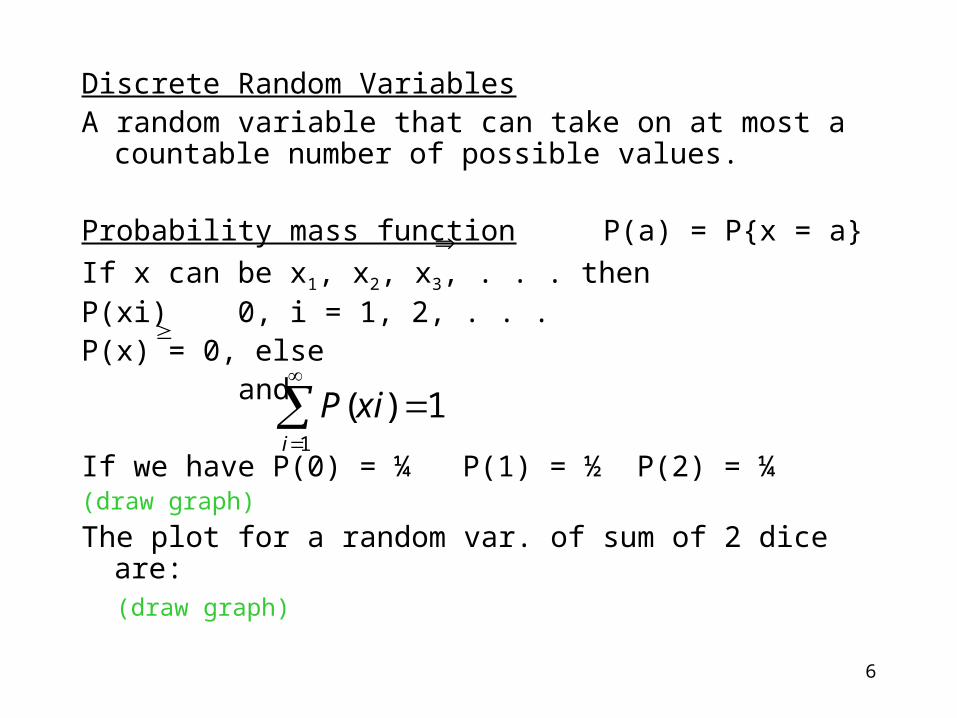
Discrete Random VariablesA random variable that can take on at most a countable

number of possible values.

Probability mass function P(a) = P{x = a}

If x can be x1, x2, x3, . . . thenP(xi) 0, i = 1, 2, . . .P(x) = 0, else and

If we have P(0) = ¼ P(1) = ½ P(2) = ¼ (draw graph)

The plot for a random var. of sum of 2 dice are: (draw graph)

1

1)(i

xiP

7

Cumulative Distr. Function F can be expressed in terms of mass function as F(a) = p(x) all x a

If x is discrete random variable where x1 x2 x3 . . . then distrib. function F is a step function. The value of F is constant in intervals [xi-1, xi) and with a step (jump) of size p(xi) at xi

Exs:x has probability mass functionP(1) = ¼ p(2) = ½ p(3) = 1/8 P(4) = 1/8

8

Then, the c.d.f is

0 a 1

¼ 1 a 2

F(x) = ¾ 2 a 3

7/8 3 a 4

1 4 a

Step size at any of values 1, 2, 3, 4 is equal to the probability that x assumes a particular value.

(draw graph)

9

Expected Value: if x is a discrete random variable with probability mass function p(x) then

expectation or expected value

This is a weighted average of possible values x can take on each value, weighted by probability that x assumes it.

If p(0) = ½ = p(1)

E[x] = 0*1/2 + 1 ½ = ½ ordinary avg. of 2 possible values 0 and 1 x can assume

Or if p(0) = ½ p(1) = 2/3 E[x] = 0*(1/2) + 1*(2/3) = 2/3 where value of 1 is given twice as much weight as value 0 so, p(1) = 2p(0) 2/3 = 2*(1/3)

0)(:

)(][xpx

xxpxE

10

Frequency Interpretation if an infinite sequence of independent replications of an experiment is done, then for any event E, the proportion of time that E occurs is p(E). So, if x can be x1, x2, x3, . . . with p(x1), p(x2), . . . then, average expectation

Exs:

Find E[x] where x is outcome of a roll of fair die

Since p(1) = p(2) = . . . p(6) = 1/6

Then, E[x] = 1(1/6) + 2(1/6) + 3(1/6) + . . . 6(1/6) = 7/2

n

i

ii xpxxE1

)(][

11

Exs

If I is a stock indicator for trading volume V then

I = 1 if V true Find E[I]

0 if VC true

Since p(1) = p(v), p(0) = 1 – p(A) we haven then E[I] = p(A)

Expected value of indicator is the probability that event occurs.

12

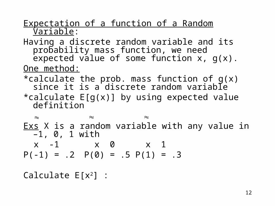
Expectation of a function of a Random Variable: Having a discrete random variable and its probability mass

function, we need expected value of some function x, g(x).One method:*calculate the prob. mass function of g(x) since it is a discrete

random variable*calculate E[g(x)] by using expected value definition

Exs X is a random variable with any value in –1, 0, 1 with x -1 x 0 x 1P(-1) = .2 P(0) = .5 P(1) = .3

Calculate E[x2] :

13

Let y = x2, it follows that prob. mass function of y is

P(y = 1) = P(x = -1) + P{x = 1} = .5

P{y = 0} = P{x = 0} = .5

hence, E[x2] = E[y] = 1(.5) + 0(.5) = .5

note that .5 = E[x2] (E[x])2 .01

14

Method 2:

if x is discrete random variable that takes on values xi, i ≥ 1 with P(xi) then for any real-valued function g,

Going back to previous example:

E[x2] = (-1)2 (.2) + 02 (.5) + 12 (.3)

= 1(.2 + .3) + 0 (.5)

= .5

i

ii xpxgxgE )()()]([

15

Corollary

if a and b are constants then E[aX + b] = a E[X] + b

Because E[aX + b] =

=

The expected value of a random variable x, E[x] is also referred to as the mean or 1st moment of x. The quantity E[xn], n 1 is the nth moment of x and, E[xn] =

0)(:

)()(xpx

xpbax

0)(: 0)(:

][)()( xpx xpx

bxaExpbxxpa

)(0)(:

xpxxpx

n

16

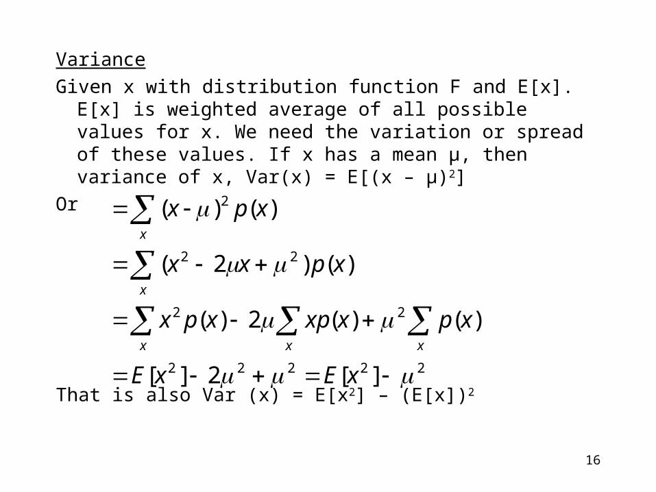
Variance

Given x with distribution function F and E[x]. E[x] is weighted average of all possible values for x. We need the variation or spread of these values. If x has a mean μ, then variance of x, Var(x) = E[(x – μ)2]

Or

That is also Var (x) = E[x2] – (E[x])2

22222

22

22

2

][2][

)()(2)(

)()2(

)()(

xExE

xpxxpxpx

xpxx

xpx

xx x

x

x

17

Exs

Calculate Var(x) if x is outcome of a fair die rolled

from previous example, E[x] = 7/2 and

E[x2] = 12(1/6) + 22 (1/6) + 32(1/6) + . . . 62 (1/6) = 91/6

Hence, Var(x) = 91/6 – (7/2)2 = 35/12

Identity: for any constants a and b Var(ax + b) = a2 Var(x)

*note that analogous to the mean being center of gravity of a distrib. of mass, Variance represents moment of inertia

*The SQRT of Var(x) is the STD. deviation of x denoted by SD(x) =

Discrete random variables are classified according to their prob. mass function.

)(xVar

18

Exs:

52-card deck is well-shuffled and then cards are turned face up one by one til Ace appears. Find expect number of cards that are face up

Let x be number cards face up til ace appears

A = { no ace among first i – 1 cards turned up }

B = { ith card is ace }

P(x = i) = P(AB) = P(B/A) P(A) =

P(x) =

)(

)(.

)1(52

452

1

481

i

i

i

49

152

1

481 116.10

)52)((

4)(

i i

i

i

i

19

Exs:

What are Expected number, Var., and S.D. of the number of spades in a poker hand? (P.H. = set of 5 cards randomly picked from 52)

A = pick any 12 spades

B = rest of cards

Thus, Var(x) = 2.43 - (1.25)2 = 0.864 and σx =

430.2)(

))((][

25.1)(

))((][

5

0525

395

1322

5

0525

395

13

i

ii

i

ii

ixE

ixE

93.864.

20

Exs

A professor made 30 exams, 8 tough, 12 medium, 10 easy; exams are mixed up and 4 are selected at random. How many will be difficult?

x number of difficult ones

We need E(x), so

x can be 0, 1, 2, 3, 4 and its probability function is

Values of all p(i.s) i 0 1 2 3 4

p(i) 0.27 .45 .24 .04 .003

E(x) = 0(.27) + 1(.45) + 2(.24) + 3(.04) + 4(.003) = 1.06

4,3,2,1,0,)(

))(()()(

304

224

8

iixpip ii

21

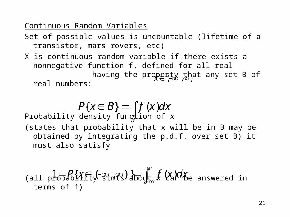
Continuous Random Variables

Set of possible values is uncountable (lifetime of a transistor, mars rovers, etc)

X is continuous random variable if there exists a nonnegative function f, defined for all real having the property that any set B of real numbers:

Probability density function of x

(states that probability that x will be in B may be obtained by integrating the p.d.f. over set B) it must also satisfy

(all probability stmts about x can be answered in terms of f)

),( x

B

dxxfBxP )(}{

dxxfxP )()},({1

22

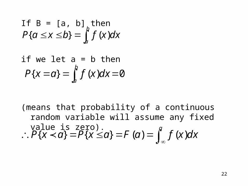
If B = [a, b] then

if we let a = b then

(means that probability of a continuous random variable will assume any fixed value is zero).

b

adxxfaxP 0)(}{

adxxfaFaxPaxP )()(}{}{

b

adxxfbxaP )(}{

23

Exs:

Suppose x is continuous random variable whose p.d.f. is

else

What is value of C?

Since f is a p.d.f., we have

and thus,

Find P(x 1)?

)24(0

2

)( xxCxf 20 x

1)( dxxf

2

0

2 1)24( dxxxC

]3

22[

32 xxC 8

3120

Cxx

1

2

1

28

32

1)24()()1( dxxxdxxfxP

24

Exs

Lifetime in days of a MEMS wireless transceiver is a random variable having p.d.f. given by

f(s) 0 x 100

100/x2 x > 100

What’s probability that 2 of 5 such devices needs replacing within 150 days of continuous operation?

25

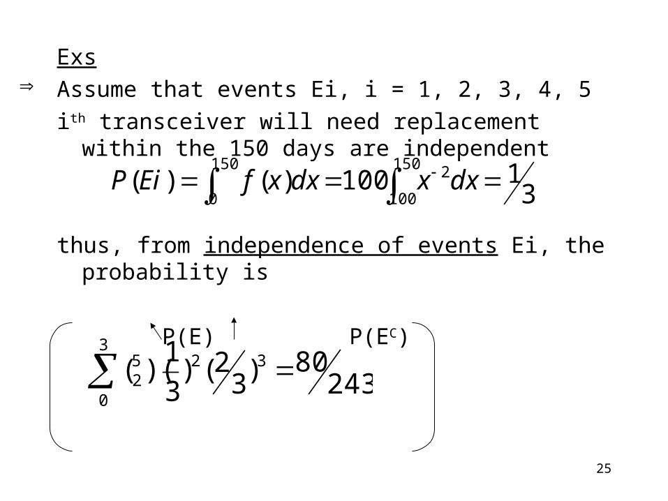
Exs

Assume that events Ei, i = 1, 2, 3, 4, 5

ith transceiver will need replacement within the 150 days are independent

thus, from independence of events Ei, the probability is

P(E) P(EC)

150

0

150

100

2

31100)()( dxxdxxfEiP

24380)3

2()3

1)(( 3

3

0

252

26

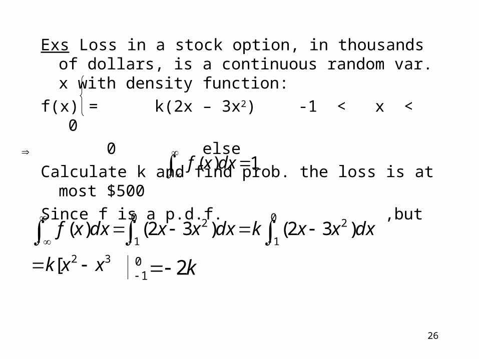
Exs Loss in a stock option, in thousands of dollars, is a continuous random var. x with density function:

f(x) = k(2x – 3x2) -1 < x < 0

0 else

Calculate k and find prob. the loss is at most $500

Since f is a p.d.f. ,but

1)( dxxf

32

0

1

0

1

22

[

)32()32()(

xxk

dxxxkdxxxdxxf

k201

27

so,

and, loss at most $500 iff x ≥ -1/2, thus

163][2

1)32(21)2

1( 0

21

3220

21

xxdxxxxP

2112 kk

28

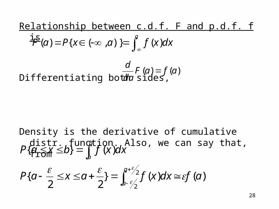
Relationship between c.d.f. F and p.d.f. f is

Differentiating both sides,

Density is the derivative of cumulative distr. function. Also, we can say that, from

adxxfaxPaF )()},({)(

)()( afaFda

d

2

2

)()(}22

{

)(}{

a

a

b

a

afdxxfaxaP

dxxfbxaP

29

Where is small and when f is continuous at x = a. In other words, probability that x will be contained in an interval of length around point a is roughly f(a). f(a) is a measure of how likely it is the random variable will be near “a”