1

1. Introduction

1.1 Wireless systems

Since the early 1980’s, wireless phone penetration has increased in an exponential manner.

Even in many developing nations, mobile phones are the dominant means of communication.

The US mobile population has grown to 190 million in 2004 [1], and is increasing. There are

several markets in developing countries that show great potential for wireless development.

Associated with this enormous customer growth is the explosion in wireless technologies and

standards. The latest generations of cellular wireless systems are designed to:

1. Enable Internet data services.

2. Provide network multimedia capability.

3. Increase voice capacity.

4. Allow for the graceful introduction of newer applications, thereby increasing the

average revenue per user.

Previous wireless systems were designed for voice-only services. With the Internet becoming

all-pervasive, users require data delivery on mobile devices. This has been the focus of

wireless research and development in recent years.

In the realm of wireless data delivery, there are 4 systems evolving at the current time -

1. Macroscopic area coverage using the cellular model: These are designed for lower

rates, but have the advantage of well defined commercial infrastructure and high

mobility. Examples are 2.5G (General Packet Radio Service - GPRS) and 3G (1

Carrier CDMA systems or 1x/cdma2000, 1 Carrier Evolution for data only or

1xEVDO, Universal Mobile Telecommunication System – UMTS and High Speed

Data Packet Access - HSDPA) cellular wireless systems.

2. Indoor wireless coverage using different Wireless LAN variants (e.g; 802.11). These

are designed to supplement the traditional Ethernet LAN and are used to cover public

Internet access areas, like airports.

2

3. Broadband Fixed Wireless Systems (e.g; WiMax or 802.16). This is designed for the

high-speed wireless backhaul. The 802.16a amendment (approved in January 2003)

specified non-LOS (Line of Sight) extensions in the 2 GHz to the 11 GHz spectrum,

delivering up to 70 Mbps at distances up to 31 miles. It is a potentially exciting last

mile technology.

4. Broadband mobile wireless access (e.g; 802.20). The goal of the 802.20 standard is

similar to 802.16e in terms of data transmission rates and range. 802.20 is targeted at

wireless metropolitan area networks for speeds around 1Mbps (to compete with DSL

and cable), with a range of up to 10 miles. In addition, it is designed for mobility up

to speeds of 155 mph.

1.2 Third generation mobile telecommunications (3G)

As defined by the IMT2000 committee, 3G is a system that offers both voice and data

services, with at least the following data rates:

V<10 kmph, d = 2 Mbps

10<V<120 kmph, d = 384 Kbps

V> 120 kmph, d = 144 Kbps

Where, V = velocity of mobile terminal and d = Physical layer data rate.

3G systems are required to provide voice quality comparable to PSTN, backward

compatibility with pre-existing networks, dynamic introduction of new services, and

asymmetric bandwidth in the downlink versus the uplink [2]. Existing wireless standards have

defined their individual paths of evolution towards 3G. IS-136 (TDMA) and GSM networks

are evolving into the WCDMA/UMTS standard, while traditional CDMA networks (i.e., IS-

95) are expected to follow the cdma2000/1xEVDO/1xEVDV migration path. It is hoped that

all 3G evolutions will eventually come together in a unified IMT-2000 standard. Figure 1.1

[3] depicts the global evolution of communication standards to the third generation. Efforts

are underway to integrate all standards into a single seamless architecture, marketed as 4G.

However, truly connected networks are many years away.

3

Figure 1.1 Evolution of mobile standards [3]

1.3 Thesis goals

In this thesis, we have used the principles of the 1xEVDO standard to design a reference

wireless system. 1xEVDO uses a scheduling mechanism with robust retransmission

mechanisms and adaptive modulation to provide high-speed data transmission in a wireless

cellular network.

We have extended the 1xEVDO design framework in an attempt to answer the following

questions -

1. How do scheduling algorithms impact user experience?

2. How do standalone transmit or standalone receive diversity interact with scheduling?

3. What is the effect of joint transmit/receive diversity and scheduling on users?

4. How does mobility affect users when scheduling and diversity is deployed?

5. What is the effect of scheduling multiple users within the same timeslot?

6. Does TCP/IP (Transmission control protocol/Internet Protocol) have an impact on

user experience over a short simulation run?

4

1.4 Similar and previous research work

Berger et al (2002) [58] studied the effect of both open and closed loop transmit diversity on a

simple PF scheduler. It was found that the cell capacity gain decreases by using dual antenna

transmit diversity. They also concluded that open loop schemes exhibit limited performance

and even loss compared to closed loop schemes over a wide range of mobility conditions.

Tse (2002) [59] proposed opportunistic beamforming to increase DL data capacity by

artificially introducing channel variations at the transmitter to increase user diversity.

Jiang (2005) [61] illustrated the interaction between the physical layer and the scheduler from

a sum-rate perspective. She proved that open loop schemes for transmit diversity reduces the

achievable sum-rate. Her work also involved optimizing downlink throughput by joint

precoding across multiple transmits antennas.

Gozali, Buehrer and Woerner [64] studied the effect of multiuser diversity on Space-time

block coding, by comparing two extreme scheduling algorithms – Greedy and Round Robin

scheduling. They used a mix of theoretical analysis and Monte-Carlo simulations to

characterize how user diversity affects system performance and to understand if multi-user

diversity mechanisms are equivalent to spatial diversity. They proved that multi-user diversity

increases both the variance and the mean of the averaged effective SNR for users; however

spatial diversity eliminates peaks in the fading channel, thus limiting the achievable

performance gain.

Kobayashi et al (2004) [60] did a recent study to quantify the tradeoffs between antenna

diversity and user diversity. In their work, transmit diversity is examined under an adaptive

scheduling policy that achieves a stability region for transmit queues. In the case of infinite

backlog of traffic, the effect of the proportional fair scheduler was studied. They proved that

in the realistic case of non-ideal data rate feedback information from the users to the base

station, transmit diversity might achieve a larger stability region and is beneficial even for

users with symmetric traffic. Their findings attenuate the common belief that channel

hardening due to transmit diversity is always detrimental for multi-user diversity scheduling

systems.

5

Except for Tse’s work that includes information theoretic results supplemented by 1xEVDO

physical layer simulation, all other studies are derived from an information theoretic

background supplemented by Monte Carlo simulations.

In this thesis, we simulate an end-to-end reference communication system using the design

principles from 1xEVDO i.e; adaptive modulation and scheduling. This reference system

closely mirrors a real world implementation, where mobiles and data cards are connected via

the wide area wireless network to servers in the core network, from which requests for data

are made. We simulate the user throughput for users on this system under various conditions.

This approach is closely tied to user experience. Several degrees of freedom are used: varying

mean channel condition for users, different scheduling algorithms, transmit and receive

diversity, etc.

1.5 Organization of the thesis

Transmit diversity, receive diversity, MIMO (Multiple Input, Multiple output) and multi-user

scheduling are described in Chapter 2. Chapter 3 dwells upon various approaches for single

user and flow scheduling. Chapter 4 briefly describes TCP and proposed enhancements for

wireless systems. Chapter 5 is dedicated to explaining the algorithms used and the co-

simulation structure between MATLAB and OPNET. In Chapter 6, we explain and interpret

the results obtained via simulation. Chapter 7 describes the conclusions reached in this study

and suggests area for future study.

6

2. MIMO and multi-user diversity

2.1 MIMO (Multiple Input, Multiple Output) systems

Till recently, commercial cellular wireless communication involved the transmission of data

between a single transmit antenna element and a single receive antenna element. Multi-

antenna systems offer potential advantages like [5] –

1. Diversity gain in fading channels.

2. Increased antenna gain.

3. Interference rejection and multipath rejection.

4. Direction of arrival determination.

5. Spatial multiplexing.

Multi-antenna systems are used for transmit diversity, receive diversity and MIMO [5].

MIMO involves the use of multiple antennas at either end of the wireless link to provide

spatial multiplexing. Multiple streams of data are sent between each transmit-receive pair,

resulting in increased data transfer. The capacity of the MIMO channel is roughly

proportional to the number of transmit or receive antenna elements, whichever is smaller [53].

Since demodulation performance can be greatly improved if the receiver obtains a less

corrupted version of the original symbol, diversity is a practical method to achieve better

system performance in wireless channels.

2.2 Temporal and Frequency Diversity

If a symbol is transmitted at different time slots, and assuming the channel is time varying,

each copy experiences a different fade. This is called temporal diversity. Due to mobility, the

complex gain of the channel varies with time. Repeating the symbol at multiples of 1/Fd,

where Fd is the Doppler spread, can ensure independent fading. Channel coding and

interleaving are used to provide temporal diversity. However, temporal diversity is not fully

effective over slow fading channels.

Frequency diversity exploits the fact that in multipath environments, different frequencies

experience different fading. Transmitting the same symbol at different frequencies ensures

7

diversity. This concept is used in OFDM (Orthogonal frequency division multiplexing),

frequency hopping spread spectrum and in rake receivers. Frequency diversity is not fully

effective over flat fading channels.

2.3 User Diversity

User diversity [7] exploits the fact that data transmission can tolerate delays and unreliability

due to different instantaneous channels seen by different users over time. The argument for

standards based on user diversity (e.g; 1xEVDO, EV-DV, HSDPA) is that there is no point in

sharing system resources with users that that cannot fully utilize the expensive air interface.

The same resources of power and code can be efficiently utilized by transmitting to users that

experience good channels. The decision to serve a user depends on –

1. The channel quality information from the receiver mobile.

2. The scheduling algorithm at the base transceiver station (BTS).

2.4 Receive Diversity

Signals from a transmitter follow multiple paths to the receiver due to reflection and

scattering from the environment. The received signal can vary widely over a few wavelengths

in a rich multipath environment. The probability of bit error (Pb) of QPSK in Rayleigh flat

fading channels is dismal; as a first approximation Pb α (Eb/No)-1, assuming no forward error

correction coding. If the receiver has access to several independent fading channels, each

carrying the same signal, it can combine the information on each path to decrease Pb at the

receiver, as seen in Figure 2.1 [8].

Figure 2.1: Effect of diversity on Pe at receiver [8]

8

A simple receive diversity combining case is shown in Figure 2.2 [8]. The fading coefficients

(α1, α2) follow independent Rayleigh/Rician distributions; w1 and w2 are weighting factors

that determine the combining algorithm. We summarize 3 linear combining schemes –

Equal Gain combining: w1=w2=1

Selection combining: w2 = 0 and w1 = 1 (|α1|>|α 2|)

w2 = 1 and w1 = 0 (|α 1|<|α 2|)

Maximal ratio combining (MRC): w1 = α 1*

and w2 = α 2*

Figure 2.2: Receive and diversity combining [8]

Other lower-complexity receive-diversity techniques include switched diversity (i.e; select

alternate antenna if current monitored antenna signal strength falls below a certain threshold).

In our simulations, we use receive diversity due to independent fading on multiple receive

antennas.

2.5 Transmit Diversity

Receive diversity is difficult to implement at a mobile due to a lack of space, power, increased

cost and the dependence on form factor. Transmit diversity moves the hardware requirements

and significant signal processing complexity to the BTS. It suffers a power penalty since the

energy from the BTS is divided between multiple antenna elements. Transmit diversity may

or may not depend on feedback from the receiver. It is usually implemented using a space-

time code, which does not require feedback. In this thesis, we do not explicitly simulate

space-time codes, but assure transmit diversity gain by using independent fading on multiple

transmit antennas with a power penalty to approximate the same.

9

Transmit diversity implementations are quite diverse, a few examples being –

1. Delay-diversity schemes: Transmissions are repeated across antennas over time.

2. Space-time trellis codes (STTC): Structure is introduced to ensure maximum rank for

code difference matrices and providing coding gain.

3. Space-time block codes (STBC): Orthogonal code structure over time provides

diversity.

4. Antenna hopping: A repetition code is transmitted one symbol at a time from nT

transmit antennas. This technique achieves diversity order = nT, using maximum

likelihood detection or maximal ratio combining at the receiver. The bandwidth

efficiency of this scheme is 1/nT [16].

2.6 Space-time codes

Figure 2.3 [9] depicts the functional diagram of a transmit diversity scheme. Well designed

transmit diversity codes attempt to achieve 3 goals –

1. Create a diversity advantage the same as maximal ratio receive combining (MRRC).

However, transmit diversity loses aperture gain due to sharing of power between the

different antenna elements.

2. Coding gain.

3. High bandwidth efficiency.

Figure 2.3: Transmit Diversity [9]

Space-time codes are open-loop transmit diversity schemes. The space-time receiver tries to

suppress the interference and decode the sub-stream received from each transmit branch.

10

There are many approaches to achieve structure in the transmitted code. The simplest method

involves linearly mapping information across nT transmit antenna elements and transmitting

these symbols in an orthogonal manner, as is done in space-time block codes. Orthogonality

can also be introduced in code using frequency multiplexing [12], time multiplexing [13], or

by using orthogonal spreading sequences for different antennas [14].

2.6.1 Space-time Block Codes [STBC]

STBC involves block encoding an incoming stream of data and simultaneously transmitting

the symbols over nT transmit antenna elements. This technique was first proposed by

Alamouti for nT = 2 and nR = 1 [11], where nR .is the number of receive antenna elements

Alamouti’s code used a complex orthogonal design, in which the transmission matrix is

square and satisfies the conditions for complex orthogonality in both space and time

dimensions. Tarokh, Jafarkhani and Calderbank [15] extended Alamouti’s code to a

generalized complex orthogonal design for nT > 2. These generalized codes are non-square,

are complex orthogonal only in the temporal domain and suffer a loss in bandwidth

efficiency.

The STBC receiver linearly processes the received symbols and uses maximum likelihood

decoding. The received signal is the linear superposition of the transmitted elements corrupted

by AWGN and Rayleigh fading. The encoder of the space-time block code is depicted in

Figure 2.4 [16].

Figure 2.4: C-STBC Transmission model [16]

At each time slot, signals cit (i=1,2,…. nT) are transmitted simultaneously from the transmit

antennas. The path gain from each transmit antenna to each receive antenna is αi,j, where i and

11

j are the element indices for the transmit and receive modules respectively. Assuming

Rayleigh fading, each path gain value is an independent complex Gaussian random sample

with zero mean and variance = 0.5 per real dimension.

The space-time block code can be represented using a k x nT matrix, where k stands for the

number of time slots used to transmit the block. The elements of this matrix consist of the

symbols transmitted such that the symbols are orthogonal to each other over time. An

example is the matrix G2 shown in Figure 2.5 [15].

Let the modulation scheme use symbols composed of b bits – hence the symbol set consists of

2b symbols. The symbols are mapped to the transmission matrix G2. In physical terms, this

matrix means that at each time slot (each row), 1 symbol is transmitted from each antenna

element simultaneously. The orthogonality between the entries in the columns allows a simple

decoding scheme. The rate of a space-time block code is defined as:

Rate = k/p (2.1)

Where, k = number of time slots required to transmit the code, p = number of symbols in the

matrix.

Figure 2.5: G2 scheme [15]

In the above example, 2 (p) symbols (x1 and x2) are transmitted in 2 (k) time slots (indicated

by 2 rows in the matrix) and hence the code rate is 1. Similarly, other codes have been

designed to work with nT = 3 [G3] and nT = 4 [G4] antenna elements [15], with rate ¾.

The STBC decoding algorithm described in this section is based on Alamouti’s scheme. The

channel is assumed to be frequency flat and slow varying. QPSK modulation is used. The

STBC decoder is depicted in Figure 2.6 [56].

12

Figure 2.6: STBC Decoder [56]

At time t, the signal rt j at the receive antenna j can be represented as –

jt

it

n

iji

jt cr

T

ηα +=∑=1

, (2.2)

where - αi,j is the fade coefficient between Tx antenna i and Rx antenna j.

ηtj is the complex channel noise at antenna j with zero mean and variance nT/2SNR

The average symbol energy is normalized so that the transmit power from each antenna is 1

and the average power at the receiver antenna element is nT. Perfect channel estimation is

assumed. The receiver computes the decision metric of Eqn. 2.3 over all the possible

codewords (l).

∑∑ ∑= = =

−l

t

n

j

n

i

itji

jt

R T

cr1 1 1

,α (2.3)

Let’s assume the G2 scheme, where only 2 complex symbols are transmitted: c1 and c2 in time

slot 1, and -c*2 and c*1 in timeslot 2. The receiver consists of a maximum likelihood receiver

where the detection rule simplifies to minimizing the following decision metric:

∑=

⎟⎠⎞⎜

⎝⎛ −−+−−

Rn

jjj

jjj

j ccrccr1

2*1,2

*2,12

2

2,21,11 αααα (2.4)

13

Due to the quasi static nature of the channel, the path gain remains the same over both symbol

transmissions. The minimizing values are the receiver’s estimates of c1 and c2 respectively.

Expanding (2.4) and deleting the terms that are independent of code words, we see that the

above minimization is equivalent to minimizing:

( )2

1

2

1,

1

2

2

2

1*1,2

*21

*,22

*2,1

*22

*,12

2,2*

1*2

*,211,1

*1

*1

*,11

)()(

)()(∑∑∑

= ==

++⎥⎥⎦

⎤

⎢⎢⎣

⎡

−+−

−+++−

RR n

j iji

n

j jj

jj

jj

jj

jj

jj

jj

jj

cccrcrcrcr

crcrcrcrα

αααα

αααα (2.5)

The above metric is composed of 2 parts:

[ ]2

1

2

1,

1

2

1*1,2

*21

*,221,1

*1

*1

*,11 )()( ∑∑∑

= ==

++++−RR n

j iji

n

jj

jj

jj

jj

j ccrcrcrcr ααααα (2.6a)

which is only a function of c1 and,

[ ]2

1

2

1,

1

2

2*2,1

*22

*,122,2

*1

*2

*,22 )()( ∑∑∑

= ==

+−−+−RR n

j iji

n

jj

jj

jj

jj

j ccrcrcrcr ααααα (2.6b)

which is only a function of c2.

The equations above may be minimized separately, and are equal to minimizing the simple

equations below, with no performance sacrifice:

( )( ) 2

11

2

1

2

,

2

11

,2

*

2*,11 1 ccrr

RR n

j iji

n

jj

jj

j

⎟⎟⎠

⎞⎜⎜⎝

⎛+−+−⎥

⎦

⎤⎢⎣

⎡+ ∑∑∑

= ==

ααα (2.7a)

for detecting c1 and

( )( ) 2

21

2

1

2

,

2

21

,1

*

2*,21 1 ccrr

RR n

j iji

n

jj

jj

j

⎟⎟⎠

⎞⎜⎜⎝

⎛+−+−⎥

⎦

⎤⎢⎣

⎡+ ∑∑∑

= ==

ααα (2.7b)

for detecting c2

Alamouti’s STBC code can be summarized as follows -

1. The code performs 3 dB worse compared with a 2-antenna MRC scheme which is

attributed to the power splitting between the 2 transmit antennas. The scheme shows

performance identical to MRC if the total radiated power is doubled.

14

2. The diversity order of the scheme is 2, the same as the 2-antenna MRC scheme.

Alamouti extended his single antenna receiver to nR receive antennas and showed that

the scheme provides a diversity order 2nR.

3. No feedback from receiver to transmitter is required.

4. No bandwidth expansion (rate = 1).

5. Low complexity decoders can be used.

Coherent STBC imposes a stringent requirement for carrier recovery and channel estimation

to compensate for phase distortion. Instantaneous tracking of phase and channel state

information is a challenging task in time varying channels. In differential STBC, information

is carried in the phase difference between consecutive symbols, hence channel estimation is

not required. Demodulation is performed by using the phase of the previous received symbol

as a noisy reference to the phase of the incoming symbol. This process may result in error

propagation. Differential space-time modulation approaches have been proposed and

investigated in [18, 19, 20, 21].

2.6.2 Space-time Trellis Codes [STTC]

STTC is a system where code, modulation and array processing techniques are jointly

designed so that the temporal orthogonality criterion may be relaxed. Traditional error

correction codes involve adding redundant bits to the bit stream, thus decreasing the

bandwidth efficiency of the transmission. In STTC, redundant information is distributed over

the space and the time domain, leading to an increased bandwidth efficiency and improved

performance for the same transmission rate.

The time multiplexing approach used in the delay diversity scheme [13] was a precursor to

such a system. In this scheme, delayed replicas of the same symbol are transmitted via

different antenna elements so that the flat fading channel becomes a frequency selective

fading channel. Tarokh and Calderbank used principles from trellis coded modulation to

create STTC [22]. STTC achieves both diversity and coding gain, but suffers from high

receiver complexity. The complexity is due to the fact that the space-time maximum

likelihood sequence estimator is often implemented as a vector-Viterbi Algorithm. Since this

code is in fact a trellis implementation, at the receiver, the trellis path with the minimum

accumulated metric is chosen. The interested reader is requested to refer to [23, 24, 25] for

further reading.

15

STTC can be summarized as follows –

1. STTC achieves diversity advantage in terms of the asymptotic slope of the BER

curves and achieves coding gain in terms of SNR offset from an uncoded system with

the same diversity advantage.

2. STTC is a proven robust scheme for slow fading environments.

3. The complexity of the decoder increases exponentially as a function of the spectral

efficiency, memory and code length of the STTC code [53].

4. Various techniques originating from TCM (Trellis Coded Modulation) can be applied

to STTC. Examples are the Calderbank-Mazo algorithm and the Generating Function

technique [10].

2.7 Multi-user scheduling, user diversity and spatial multiplexing using THP

We know that adaptive modulation and coding helps increase data rate and spectral efficiency

in wireless systems. Another such technique is known as “pre-coding”. Tomlinson and

Harashima introduced pre-coding as a technique for ISI mitigation in the 1960s [26]. Their

structure is referred to as the Tomlinson–Harashima Pre-coder (THP).

To understand THP, let’s revisit the decision feedback equalizer (DFE) depicted in Figure 2.7

[27]. DFE is a widely used method to mitigate ISI. The DFE consists of a feed-forward filter

to whiten noise and yield a minimum–phase response. This response is inverted with a

feedback filter driven by detected symbols. In THP, the feedback filter is placed at the

transmitter, as shown in Figure 2.8. The feedback filter has a transfer function that inverts the

channel impulse response and pre-equalizes the data. THP requires advance knowledge of the

channel transfer function. For this purpose, it is necessary to continuously update the

transmitter about the channel state information by means of a feedback channel. Since

feedback channels are readily available in present-day wireless standards, pre-coding has

received renewed attention because of its superior performance over DFE in coded

communication systems. One drawback of THP is that any mismatch between channel

prediction and the true channel causes an unacceptable amount of ISI at the input of the

receiver detector. The mismatch depends on Doppler spread. The ISI at the detector input can

be compensated with a conventional Linear Equalizer (LE). Castro and Castedo [28] showed

that the performance of the overall pre-coding scheme is limited by the normalized Doppler

frequency.

16

Multi-user interference cancellation is similar to ISI cancellation. Since the previously

transmitted symbols are known at the transmitter, the interference is known if the transmitter

has knowledge of the channel. This is another way MIMO and frequency selective channels

are connected. THP was devised as an alternative to receiver-based DFE for the frequency-

selective channel; the analog to a SIC receiver in MIMO and uplink channels. In flat fading

channels, THP can be applied to a MISO (multiple input and single output) broadcast channel

as a transmitter version of the V-BLAST algorithm [29]. THP promises to be a spectrally

efficient transmission scheme without error propagation, unlike the DFE structure.

Figure 2.7: Decision Feedback equalizer [27]

Figure 2.8: Precoding and decoding with Tomlinson-Harashima equalization [28]

17

To further explain this technique, consider a spatial zero-forcing T-H precoding system that

forms a distributed MIMO system as shown in Figure 2.9 [29]. The transmitter at the BTS has

nT transmit antennas, and K receive antennas are distributed between K receivers, with one

antenna element per receiver. At each time slot, the BTS schedules nS users, where nS ≤ nT.

The BTS sends a data packet to each of nS users. Maximum spatial multiplexing gain occurs

when nS = nT . Let H(S) be the channel matrix between nT transmit antennas and nS scheduled

users. Each element of the matrix is a complex Rayleigh fade coefficient with unit variance.

Assume that the total BTS transmit power PT is equally split among the nS users. Each

receiver performs maximum-likelihood detection. White complex Gaussian noise (ñi, i =

1,…,ns) with mean = 0 and unit variance is added at the receiver input of each of nS users.

Figure 2.9: Distributed MIMO system [29]

Based on this ZF-THP model, the downlink channels are decoupled into nT independently

faded channels with SNR = TiTi ngP /2=ρ (i = 1,2,…n) and the received signals can be

expressed as:

( ) TM

iTTiiMgnP

iiiTT nignPnanagnPriiiTT

..2,1,///~

/

~~

=⎥⎦⎤

⎢⎣⎡ +=⎥⎦

⎤⎢⎣⎡ += (2.8)

Where – gi = Central chi-square random variables with 2(nt-i+1), i = 1,…nT degrees of freedom.

Mi = element in the modulus vector M = [M1, M2, … Mns]T

Consequently, Jiang shows that the achievable rate for the user’s channel is:

HzbpsnignPnhMnPR TMiTTiiTTzfthpi i

/....2,1),)]//(([)2(log2)/(~

2 =−= (2.9)

18

Jiang further extends the theory under the following assumptions:

1. Uniformly distributed signals over a square Voronoi region

2. The input SNR is available and hence noise cooling can be characterized.

3. Modulo loss ignored.

4. Equal power allocation across all transmit antennas.

She proves that the achievable sum rate for ZF-THP is –

∑∑==

−+−==tt n

iiisTii

n

isT

zfthpisT

zfthpsum xgnPnhnPRnPR

12

1

)]])~1(//(~([2)6([log)/(~

)/(~

23

αα (2.10)

(bps/Hz)

Where, α = (PT/ nT)(1+ PT/nT)

n = zero-mean real Gaussian random variable of variance 0.5.

x = real random variable uniformly distributed over [- (3/2)1/2 , - (3/2)1/2]

h(.) = The differential entropy function.

With a large number of users K>nT, the maximum sum rate is achieved through multi-user

selection -

zfthpsum

S

zfthpsum RR

~max

~ max =− (2.11)

… over all ordered user subsets S with cardinality | S | ≤ nT.

For THP, a greedy scheduler is one that maximizes the sum rate for ZF-THP. The greedy

scheduler ignores fairness of time-slot allocation to users, thus a proportional fair (PF)

scheduler brings about a balanced tradeoff between multi-user diversity and fair allocation of

time slots. The PF scheduler is extended in [29] for multi-user transmission, and assigns a slot

to the user subset satisfying –

∑=

=sn

i i

i

S tT

tRS

1

*

)()(

maxarg (2.12)

Where – Ri(t) is the achievable rate of the user in slot t

Ti(t) is the average throughput over a past window of length Tc.

19

Ti(t+1) = (1-1/ Tc)Ti(t)+ Ri(t)/Tc *Si ∈

(1-1/ Tc) Ti(t) otherwise

For greedy scheduling, a maximization of the sum rate requires TnKP number of subsets to

determine the scheduled set for that time instant. TnKP is a permutation of nT (# transmit

antennas) over K (# users). Jiang [29] proposes a sub-optimal scheduler with maximum

spatial multiplexing and equal power allocation. In this suboptimal scheduler, the total

number of subsets for which the search is performed reduces to –

2/)12( +−= TTi nKnN (2.13)

Consequently, the steps carried out to schedule the list of users at a particular time instant are

shown in Figure 2.12 [29].

Figure 2.12: Suboptimal GD scheduler with equal power allocation and maximum spatial

multiplexing [29]

20

3. Scheduling for packet data

3.1 The definition of scheduling

Scheduling is a method of allowing multiple users to share a common resource. In the

wireless context, scheduling allocates systems resources (for e.g; transmit power, bandwidth,

modulation scheme), to optimize a measure of goodness (for e.g; throughput, delay).

Scheduling was traditionally used in applications like the allocation of CPU resources

between tasks in operating systems. The sophisticated algorithms developed for these systems

are nowadays applied in the wireless arena to schedule packets to users.

Scheduling in the downlink of a wireless, time-slotted system is a two-pronged problem. The

first problem is that of user scheduling, i.e; “which user(s) should be served in time slot x?”.

The second problem is that of selecting between flows, i.e; “If I have n different types of

traffic directed to a single user, which traffic flow should get served in timeslot x?”. For

completeness, we have described algorithms needed for both scheduling requirements.

Unlike voice, data is typically delay insensitive. Exceptions to this statement are the cases of

streaming live video or speech over data packets. Data systems can exploit fading channels by

using scheduling algorithms. Tse [30] proved that the best strategy to maximize system

throughput is to transmit to users who see the best channels if fading gains are tracked at the

receiver and sender.

An important scheduling criterion is one of fairness. For example, if the base station always

serves the user with the best channel, poor-channel users would be starved. Hence, algorithms

need a way of balancing the scheduled users. In this thesis, we concentrate on scheduling

users on the downlink by comparing the effect of 3 different scheduling algorithms –

1. Greedy (GD) scheduling

2. Round Robin (RR) scheduling

3. Proportionally Fair (PF) scheduling.

These algorithms are used to decide the user to schedule during a given slot.

21

3.2 Scheduling between users

Consider the class of algorithms that may be used to schedule users in the downlink [33]:

1. Round robin scheduling (RR) - Users are chosen in cyclic order for transmission,

regardless of their individual requested rates, unless a user is in outage (i.e; the user

cannot support any granular rate). This algorithm provides the highest degree of

fairness with respect to the air interface, but suffers low average throughput, since

channel conditions are ignored.

2a. Greedy Scheduling - In this strategy, the scheduler selects a user who reports the

highest C/I ratio. This provides the maximum possible average throughput per sector.

2b. MaxD - The maximum DRC (Data Rate and Coding) algorithm is a variation on the

greedy scheduling strategy. The C/I received by the user is divided into many ranges

and each is represented by a single integer value called the DRC. The transmission

rate is proportional to the DRC, and there can be reduction in optimal throughput due

to the quantization of the received C/I ratio.

3. Proportionally fair scheduling: In the PF scheduling algorithm, provisions are made

so that bad channel users are not starved. The definition of fairness in PF scheduling

is as follows: If, by using another scheduling algorithm, the throughput for user i

increases by x%, then, the net decrease in throughput for all the other users in the

systems in more than x%. [54].

The PF scheduler serves the user with the highest value of DRCi(t)/Ri(t).

where – DRCi(t) is the data rate requested by user i at time t

Ri(t) is the average throughput at time t for the user i over the given window.

Ties are broken randomly. Any user that has no data to send is ignored in the

calculation. The scheduler works as follows:

a. Initialization: At time slot t = 0, set Ri(0) = 0 for all i.

b. For 1 ≤ i ≤ K, Ri(t) is exponentially averaged in every slot. The averaging

time constant is dictated by tc.

c. Updating: For i = 1:K

Ri(t + 1) = (1 - 1/tc) · Ri(t) + 1/tc · Ii(t) (3.1)

22

Where - Ii(t) = the current rate of transmission for user i if it is served in time slot t,

else 0.

tc = time constant for long term exponential averaging to update Ri(t).

The PF algorithm provides fairness by ensuring that all links get equal airtime. Assume 2

users scheduled on a link with the peak rate of one user thrice that of the second. If we plot a

graph of the service amount vs. time, we see that the slope of the higher rate user is thrice that

of the lower rate user. The proportionally fair (PF) scheduling algorithm is used in 1xEVDO

[31], [32].

In a more general scheme, the scheduling decision is made based on the user who has the

highest value of Ri(t), instead of DRCi(t)/Ri(t). Other hybrid schemes have been proposed in

literature. Examples of these are MaxD/PF scheduling and the M-LWDF algorithm (Longest

Weighted Delay First) [33].

3.3 Scheduling between transactions

A common usage scenario is when the user opens multiple applications each using multiple

transport layer (TCP/UDP) sockets. For example, a user might have an HTTP connection

open in parallel with a file transfer and a streaming video. This means that flows to the same

user must be scheduled at the base station depending on the priority of packets belonging to

each flow. At every slot, the system must make a decision on which job to serve. These

algorithms are broadly classified as EDF (Earliest deadline first) or PS (processor sharing)

algorithms. These algorithms are described in detail in [34].

3.3.1 EDF (Earliest Deadline First) Algorithms [34]

EDF algorithms serve jobs that have the earliest expiring deadline. Examples of EDF

algorithms are -

1. SRPT (Shortest Remaining Processing Time): In this strategy, jobs that have the least

remaining processing time are served first. This strategy minimizes the mean

response time if the scheduler is aware of the transaction length of each job.

2. FB schedulers (Foreground Background schedulers): In this strategy, the job that has

received the least service is scheduled for delivery in the next eligible slot. This

scheme statistically approximates the SRPT scheduler.

23

3. SRJF (Shortest Remaining Job First): As the name indicates, the scheduler schedules

a job that has the least amount of data left to be processed (sent).

4. FIFO (First In First Out): Jobs are served depending on the time at which they arrive

at the scheduler.

While the above schemes are simple, other complex algorithms based on the concepts of flow

and stretch are proposed in [34].

3.3.2 PS (Processor Sharing) algorithms [34]

A second category of algorithms that schedule between flows are called processor sharing

techniques. Examples of PS algorithms are -

1. The Bit Proportional algorithm: The power assigned to the job in the downlink is

proportional to the size of the job in bytes. The larger the size of the job, the larger is

the resource given to it.

2. The Work Proportional algorithm: The weight assigned to a job is proportional to the

energy required for the job. If Pmax is the total power available at the BTS, Rmax is that

maximum rate available to the job and |Ji| is the size of the job in bits, the power

assigned to the job is proportional to the energy required for the job i.e; Pmax x

|Ji|/Rmax.

3. The Work Processor Sharing algorithm: The power assigned to each job is

proportional to the energy per bit (Pmax/Rmax). This is the work proportional algorithm

(PS algorithm 2), without dependency on the size of the job.

4. The Uniform Processor Sharing algorithm: Power is equally shared among all jobs.

Joshi, Kadaba, Patel and Sundaram [34] proved that processor scheduling is not effective for

practical wireless systems due to quantized channel quality feedback.

3.4 1xEVDO [35]

CDMA 1x-EVDO (CDMA 1-carrier Evolution for Data Optimized services), also called

High Data Rate (HDR) or IS-836 is a packet data standard developed at Qualcomm Inc. HDR

is conceptually different from other standards since it only supports data. HDR provides a

theoretical packet data bit rate of up to 2.47 Mbps on the forward link. To obtain such high bit

rates in the narrow 1.25 MHz band, the proposal uses novel techniques like -

24

1. Channel quality feedback: Frequent estimation and prediction of the radio channel is

fed back to the base station.

2. Adaptive modulation and coding (AMC): The modulation scheme is changed

depending on the quality of the channel reported by the user.

3. Hybrid ARQ (Hybrid Automatic Repeat Request): Information bits are first encoded

by a low rate mother code. The information bits and selected parity bits are then

transmitted. If the transmission is unsuccessful, the transmitter sends additional

selected parity bits. The receiver soft combines the new bits and those that were

previously received. Each retransmission produces a stronger code [55].

4. Scheduling: Proportionally Fair scheduling is used for fairness among users.

The system supports data rates in several granularities: 38.4, 76.8, 153.6, 204.8, 307.2, 614.4,

921.6, 1800, 1600 and 2400 kbps on the downlink, using QPSK, 8PSK and 16QAM

modulation. Depending on the data rate, a forward link packet may occupy between 1 and 16

time slots. Power control and handoff are not used on the forward link. Instead, all time-

multiplexed packet transmissions occur at full power. The best serving sector is selected by

the mobile user instead of handoff (this is the scheduling algorithm 2a in section 3.2). AMC

and hybrid ARQ are employed to take full advantage of the available SINR. Turbo coding is

used for error correction. Packet transmission is done in 1.67 ms time slots, with only one

user receiving data in a given slot. Sector throughput is increased by proactively scheduling

users with favorable channel conditions. The mobiles or access terminals (AT) estimate their

received SINR from a pilot signal transmitted by the base station. Each AT measures the

received SINR, and makes an decision on the bit rate and transmission format that can be

supported on the forward link with an average 1% packet error rate (PER). The SINR value is

mapped to a number called the data rate and coding (DRC). The mobiles communicate the

DRC to the BTS in terms of a 4-bit request to the base station over a dedicated reverse link

channel. In our simulation, the SINR feedback is assumed to be error-free. The scheduler at

the base station decides the user to be served on the basis of this feedback value. The

scheduler sends data to the AT that has the highest DRC/R value (PF algorithm). DRC is the

rate requested by the mobile while R is the average rate received by the mobile over a window

of appropriate size, i.e; the scheduling algorithm 3 in section 3.2.

25

4. TCP modifications for wireless systems

Since most Internet traffic is carried over TCP (Transmission Control Protocol)/IP (Internet

Protocol), the seamless interaction between TCP/IP and lower layers in new wireless

networks is important. While IP is responsible for routing, TCP is a transport-based,

connection-oriented, end-to-end reliable protocol [48]. Many results in this thesis are

compared with respect to the user’s received TCP throughput.

4.1 Acknowledgements and reliability using acknowledgements (ACK)

TCP ensures that the data received at the receiver is exactly the same as the transmitted byte

stream. In response to received packets, ACKs are generated. When an ACK arrives, the

sending TCP module determines if it is the first ACK or a duplicate ACK (DUPACK) for the

sent segment. If it is the first ACK, the sender deduces that all bytes up to the value indicated

by the ACK have been received. The sender increments the state variable keeping track of the

bytes (in terms of sequence number; SN) that the receiver has acknowledged. DUPACKs are

generated when the receiver obtains a packet with a SN larger than the next expected in-order

sequence number. This is a gap in the byte stream. TCP does not use negative

acknowledgements (NAKs) to signal a loss of a packet, instead, sends a DUPACK for the last

in-order byte received. If another gap is detected, the receiver sends a second DUPACK. At

this point, the sender has received 3 ACKs for the same segment. At this point, the sender

side TCP assumes that there is a high possibility that the segment following the

acknowledged packet is lost.

4.2 Flow control

When a TCP connection is set up between 2 hosts, each peer entity allocates a receive buffer

for the connection. The application reads segments from the buffer. If the application is slow,

the receive buffer could overflow. Flow control is used to alleviate the problem – it ensures

that the sender never sends more data than that can be handled at the receiver. The receiver

advertises the receive window, RcvWin to the sender. RcvWin (Figure 4.1) dynamically varies

in size during the lifetime of the connection.

26

Figure 4.1: Receive Window

RcvWin = RcvBuffer – [LastByteRcvd - LastByteRead] (4.1)

Where - RcvWin - Advertised window

RcvBuffer - Size of receive buffer

LastByteRead - The last byte that was read out by the application layer

LastByteRcvd - The last byte received from the sender by the receive buffer.

RcvWin size is sent out with every ACK. Initially, RcvWin = RcvBuffer. The sender keeps

track of the LastByteSent and LastByteAcked. The difference between LastByteSent and

LastByteAcked is the number of bytes “in-flight”. By keeping this value less than RcvWin,

flow control is achieved.

4.3 Round trip time (RTT) and Retransmission time out (RTO)

Every segment sent experiences a finite round trip time (RTT) before it’s ACK can be

received. For each segment, a timer is started, the timeout for which is called the

retransmission timeout (RTO). RTO is updated from the RTT experienced by TCP segments

on the connection. Each time the RTT variable is updated, RTO is recalculated based on a

smoothed estimate called Jacobson-Karels smoothing -

RTO = max (RTO_min, R+4V) (4.2)

V 3/4 V +1/4 |R-RTT| (4.3)

R 7/8 R + 1/8 RTT (4.4)

27

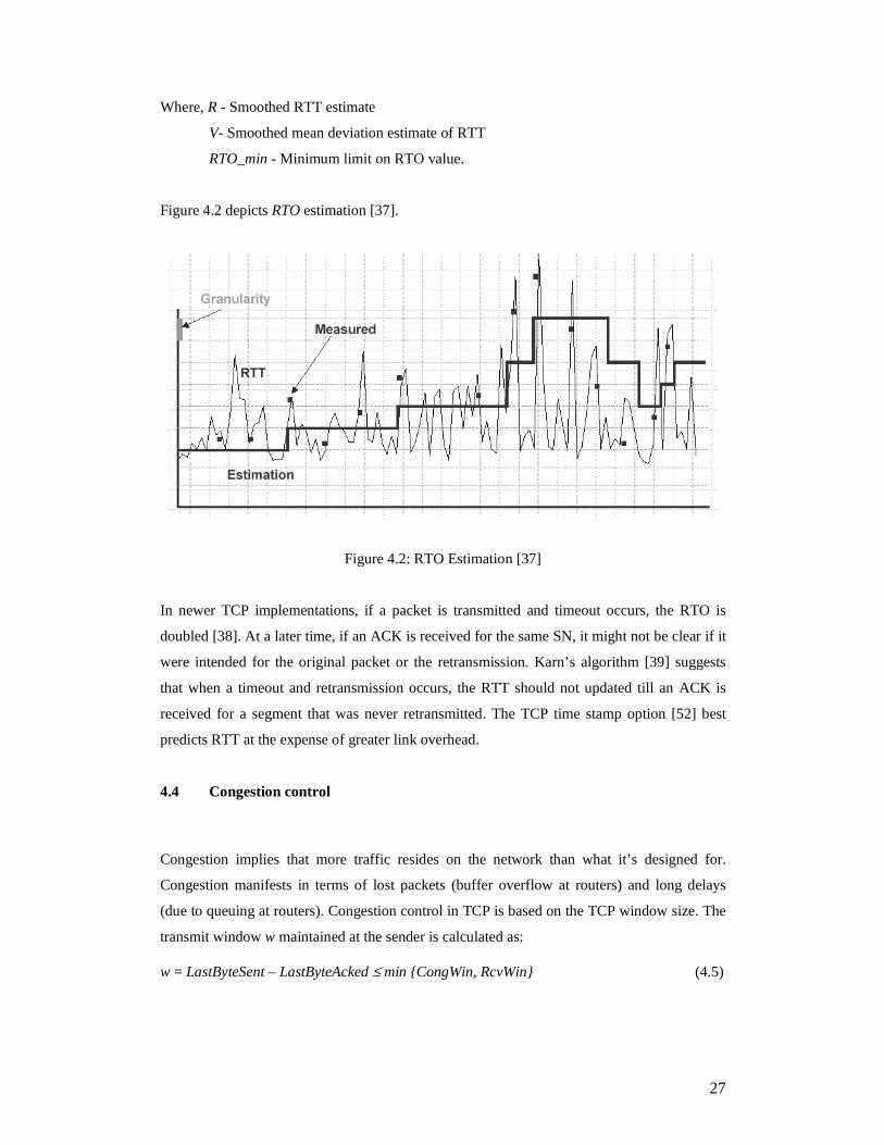
Where, R - Smoothed RTT estimate

V- Smoothed mean deviation estimate of RTT

RTO_min - Minimum limit on RTO value.

Figure 4.2 depicts RTO estimation [37].

Figure 4.2: RTO Estimation [37]

In newer TCP implementations, if a packet is transmitted and timeout occurs, the RTO is

doubled [38]. At a later time, if an ACK is received for the same SN, it might not be clear if it

were intended for the original packet or the retransmission. Karn’s algorithm [39] suggests

that when a timeout and retransmission occurs, the RTT should not updated till an ACK is

received for a segment that was never retransmitted. The TCP time stamp option [52] best

predicts RTT at the expense of greater link overhead.

4.4 Congestion control

Congestion implies that more traffic resides on the network than what it’s designed for.

Congestion manifests in terms of lost packets (buffer overflow at routers) and long delays

(due to queuing at routers). Congestion control in TCP is based on the TCP window size. The

transmit window w maintained at the sender is calculated as:

w = LastByteSent – LastByteAcked ≤ min {CongWin, RcvWin} (4.5)

28

The congestion window (CongWin) is initialized at small value, typically 1 MSS (Maximum

Segment Size = size of TCP payload). As the connection progresses and ACKs arrive in

regularity, CongWin increases till it reaches RcvWin.

Following the initialization process, TCP follows a behavior called slow start -

1. Initially, CongWin = 1 MSS. A TCP packet is sent, and the ACK is received within 1

RTT. Cycle 1 ends.

2. In slow start, CongWin = 2 MSS.

3. 2 TCP segments are sent, and 2 ACK’s are received within the next RTT.

4. In slow start, TCP increases the transmit window by 1 MSS for every ACK.

5. At the end of the second cycle, CongWin = 4 MSS.

This continues till CongWin equals another variable called the slow start threshold or

ssthresh, after which, CongWin increases by 1 MSS each RTT. This phase cautiously

increments CongWin and is called the congestion avoidance phase. Congestion avoidance

continues as long as ACKs for segments arrive before timeout expiry. If no congestion occurs

on this path the transmit window will hit the advertised RcvWin and grow no further. If any

packet sent gets lost and the RTO expires, TCP updates the connection variables as –

1. ssthresh = ½ x CongWin

2. CongWin = 1 MSS

TCP evokes slow start yet again. The version of TCP just described is called TCP Tahoe.

Figure 4.3 [37] depicts the window growth in TCP Tahoe.

Figure 4.3: TCP Tahoe window behavior [37]

29

In terms of the Round trip time (RTT) and MSS, TCP throughput is expressed as –

TCP_Throughput = w x (MSS/RTT) bytes/sec (4.6)

Where, w -Transmit Window Size.

The slow start mechanism causes a large drop in TCP throughput. To overcome this, a

concept called fast retransmit is used in TCP Reno. When a packet is lost, the receiver keeps

sending a DUPACK for the last in-order segment received. Instead of waiting for the timer to

expire, the sender retransmits the segment on receipt of the third DUPACK and updates the

connection variables as follows -

1. Upon 3 DUPACKS: CongWin CongWin/2 and initiate congestion avoidance.

2. Upon RTO: ssthresh = ½ CongWin and initiate slow start with CongWin = 1 MSS.

If the RTO expires, TCP Reno goes back to slow start. This is a judicious thing to do, since

RTO is an indication of extreme congestion in the network, or wireless link outage (likely in a

handoff between 2 different wireless systems like between WCDMA and GPRS). The

advantage of this scheme is that slow start is avoided when the 3rd DUPACK is received.

Figure 4.4 depicts window behavior in TCP Reno [37].

Figure 4.4: TCP Reno window behavior [37]

4.5 Support protocols for TCP in for wireless systems.

Wireless channels can fail to deliver packets if suitable redundancy schemes are not

employed. When a packet gets lost or corrupted, the TCP module at each end has no way of

knowing that the packet was lost over the air. TCP falsely assumes that packet error is due to

30

congestion, and fires off the congestion control algorithms. A general wireless network is

shown in Figure 4.5, where mobiles are connected to a core network. Wireless links typically

show packet error rate (PER) ~ 10-6 or worse, which is unacceptable for good TCP

performance. To decrease PER on the wireless link, a second hierarchy of protocols is used in

addition to TCP/IP. For eg, in 1xEVDO/CDMA2000, this protocol is called RLP (Radio Link

Protocol) while in WCDMA/UMTS this is called RLC (Radio Link Control). In this thesis,

we have simulated a simple NAK based RLP protocol.

Figure 4.5 General cellular wireless data network

TCP/IP packets are broken into smaller RLP packets at the sender module before they are sent

over the air. RLP performs local retransmissions in case the packet is lost. RLP hides the

fragility of the wireless channel and presents TCP with a low PER link. Farid [40], showed

that as long as the frame errors are i.i.d, the RLP mechanism proposed for CDMA2000

performs well for frame errors of up to 20%.

RLP needs to be carefully designed so as to ensure the following -

1. TCP timing mechanisms remain unaffected.

2. RLP remains transparent to TCP.

3. TCP ACK timing remains unchanged irrespective of the underlying protocol.

4.6 Proposed techniques of improving TCP behavior in wireless systems

The deployment of data capable wireless systems is the driving force for TCP performance

enhancements. This section summarizes various optimizations proposed in literature [41].

31

1. I-TCP [42] - Split the path between source and destination into a wired and wireless

part. TCP retransmissions are done from the interface between the two domains.

2. Partial Acknowledgment algorithm – Use two different types of ACKs to distinguish

losses in the wired versus the wireless network. The fixed sender needs to handle the

two types of acknowledgements differently.

3. Supplemental Control Connections – Create a control connection that terminates at

the BTS. Packets are sent periodically on the connection to measure the congestion

status of the wired network, using which a decision as to the real cause of packet loss.

4. Explicit Loss Notification (ELN) - Use bits in the TCP header to communicate the

cause of packet losses to the sender.

5. Snoop protocol [43, 45, 46, 47, 48] – A method to make TCP a link-aware scheme. It

introduces a snooping agent at the BTS to observe and cache TCP packets directed

to/from a mobile. By snooping the ACKs, the agent can determine which packets are

lost on the wireless link. The snoop agent performs local retransmissions. DUPACKs

due to wireless losses are suppressed to avoid triggering end-to-end retransmission

from the source. The snoop protocol finds the exact cause of packet loss and takes

actions to prevent TCP from starting the congestion control algorithm.

6. Hiding enhancements - Attempts to hide wireless losses from TCP. Hiding assumes

the use of an RLP type protocol to build a reliable link layer. Studies show that a

reliable link layer via retransmissions achieves good TCP performance. When hiding

approaches are used, TCP settings need to be tweaked. For e.g; in [40] the authors

have modeled RTT and adjusted the RTO value for CDMA2000.

7. SACK (Selective acknowledgements) - [49] demonstrates the strength of SACK over

non-SACK implementations. SACK option is useful when multiple, non-adjacent

packets are lost from one window of data. In TCP, the sender can learn only about a

single lost packet per RTT. In SACK, the receiving module explicitly notifies the

sender of missing packets, so the sender only retransmits the missing data [50].

In this thesis, we implement mechanisms 6 and 7. We use RLP as a hiding mechanism to

mask the high BER physical layer. In addition, we use set up the simulation environment so

that the server and the mobiles can support SACK and TCP timestamps. The SACK and TCP

timestamp algorithms are directly taken from the OPNET modeler implementation. The TCP

timestamps options allows for accurate estimation of RTT at the expense of larger header

overhead.

32

5. Simulation model and strategies

5.1 Overview

This chapter describes the co-simulation and algorithms implemented using OPNET Modeler

10.x [51], MATLAB [6] and C++. The physical layer components, i.e; Rayleigh fade

generation, SNR estimation for different combinations of receive/transmit antennas and THP

were implemented in MATLAB. The higher layers i.e; RLP and the scheduler were written in

C/C++, using the kernel procedures available within OPNET. OPNET’s default TCP/IP stack

was used but was configured using the handles provided by the software package.

5.2 The concept of co-simulation

With the increasing complexity of algorithms proposed for each layer in a communication

stack, optimizing one layer may result in deleterious effects on the overall system. A new

paradigm in wireless design calls for the joint design across all layers of the communication

stack to support various and changing traffic types; each with a different quality of service.

This is called cross layer design [17], [43].

The results are presented in terms of the throughput experienced by each of the users in the

system. We also plot the total bytes served by the network on the downlink or the total

throughput experienced by all the users on the system, based on the simulation scenario. In

this thesis, we evaluate the joint effect of the following components in the reference wireless

system –

1) Transmit diversity alone or receive diversity alone or both

and

2) Single user scheduling or multi-user scheduling

and

3) Symmetrically distributed users (users given the same mean channel) or

asymmetrically distributed users (different users given different mean channels).

Asymmetric users are also referred to as well-distributed users.

4) Loaded or non-loaded system

33

5.3 System simulation model in OPNET/MATLAB/C++

Figure 5.1 is an example of our network model with 4 users in the sector. The simulation is

scalable to 3 sectors with 60 users per sector and multiple servers, each offering different

traffic types. In order to calculate user throughput over the simulation run, a non-bursty

application is implemented at each mobile. All users make data traffic requests at the

beginning of the simulation run. The required TCP/IP sockets are opened between the server

and the client and traffic is sent from the server to the client.

Figure 5.1: System simulation model

The focus of this simulation effort is forward link performance. An ideal link reverse link (no

loss) is assumed. This reverse link simulated is also associated with zero delay. This tends to

reduce the RTT that might be seen in a real world system. The BTS contains the scheduler

and RLP stack. The BTS is connected to the PDSN (Packet Domain Switched Network). In

the simulation, the PDSN sniffs the TCP/IP packets due to each of the users. The packets are

marked with simulation parameters associated with each of them (e.g; information about

source and destination IP address) before they are forwarded on to the BTS or back to the

server.

At every scheduling instant (1.67 ms), the MATLAB code generates fade coefficients for

each user. Jakes sum of sinusoids (SOS) model is used [44]. This channel quality information

34

is fed back to the BTS. The BTS scheduler schedules RLP packets to a user based on the

selected scheduling algorithm (PF, GD, RR). The channel feedback dictates the modulation

scheme used at that scheduling instant for the scheduled user.

Figure 5.2 depicts the BTS. The scheduler resides in module p_0. Each queue in the BTS

(q_*) stores the RLP packets for each user. The queue is interrupted by the scheduler when

the scheduling decision is made. The MATLAB interface code resides in the user module

(user*). Each user module leads to a wireless transmitter block (rt_*). At the receiver, each

packet captured is by a wireless receiver (rr_*) (Figure 5.3). The wireless receiver contains

the receive pipeline available in OPNET. Packets that are correctly demodulated are sent to

the rlp_reassembly block where the RLP packets are re-assembled into TCP/IP packets.

These packets are sent to the application that requested them.

Figure 5.2: The BTS

35

Figure 5.3: The wireless receiver

5.4 Generating Rayleigh fade coefficients

Consider the transmitted signal s(t), received signal r(t) in a Rayleigh flat fading channel.

r(t)=s(t)γ(t)+n(t) (5.1)

γ(t)=a(t)+jb(t) (5.2)

Where a(t) and b(t) are both Gaussian distributed, with zero mean and variance = 0.5 per

dimension.

The amplitude of the fading distribution has a Rayleigh distribution.

γ(t)=R(t)ejθ(t) (5.3)

The envelope pdf of the carrier in an environment with no LOS is given by Rayleigh

distribution -

2/2

)( rR rerf −= , r > 0 (5.4)

The phase (θ) pdf is given by the uniform distribution –

πθ

21

)( =Θf , 0 ≤ θ < 2π (5.5)

In the case of SOS simulators, the received signal is characterized by the sum of randomly

phased sinusoids. The Rayleigh fading value is added in dB to the meanSNR value assigned to

36

each user. This is the final channel strength seen by the user. Appendix A shows the code

snippet that generates Rayleigh fading. The code snippet shows how transmit and receive

diversity are accounted for by summing and normalizing multiple Rayleigh channels.

5.5 Transmit and receive diversity implementation

Assume 2 transmit and 2 receive antenna elements. We generate 4 independent Rayleigh fade

channels -

γ11 tx #1 rx#1

γ12 tx #1 rx#2

γ21 tx #2 rx#1

γ22 tx #2 rx#2

For transmit diversity there is no power gain since transmit power stays constant and is split

across antennas. Receive antennas double the total available power. (3dB improvement).

Assuming no Tx diversity and only Rx diversity (2 receive antennas) -

Total_receiver_signal = γ11+γ12

Assuming 2 Tx antennas and 2 Rx antennas -

Total_receiver_signal = (γ11+γ12+γ21+γ22)/(21/2)

5.6 Generation of BER curves

At the receiver, a decision is made as to whether the received RLP packet can be decoded. We

first generate the BER curves in MATLAB and convert the values into a format that OPNET

can access. We assume that –

1. The packet experiences flat fading since the duration of the slot is 1.67 ms. Hence, the

BER curves generated include only the effect of AWGN.

2. Convolutional coding is used with rate r = ½ and constraint length k = 7.

We use the method outlined in [23] to generate the BER curves for the specific modulation

scheme with coding.

37

⎟⎟⎠

⎞⎜⎜⎝

⎛=

< ∑∞

=

o

bd

ddddb

N

dREQP

PcPfree

2 (5.6)

where – cd : coefficients taken from [24].

Pd : bit error probability in AWGN for a given modulation scheme

R : code rate

d : free distance

For 8-PSK, Pd is modified as in Eqn 5.6a.

⎟⎟⎠

⎞⎜⎜⎝

⎛=

o

bd N

dREQP

88.0 (5.6a)

For M-ary QAM, the general result for Pd is

⎟⎟⎠

⎞⎜⎜⎝

⎛=

o

Mbd N

dREQP

η22 (5.6b)

where – η M is a correction factor.

For each of the above, d varies from 10 to 17 to account for the free distance. Finally, the bit

error rate calculation for each modulation scheme is shown below –

Pb-QPSK (i)= 36*Pd-QPSK (1) + 211* Pd-QPSK (3) +1404* Pd-QPSK (5) + 11633* Pd-QPSK (7) (5.7a)

Pb-8PSK (i)=36* Pd-8PSK (1) + 211* Pd-8PSK (3) +1404* Pd-8PSK (5) + 11633* Pd-8PSK (7) (5.7b)

Pb-16-QAM(i)=36*Pd-16QAM (1) + 211*P d-16QAM (3) +1404*P d-16QAM (5) + 11633*P d-16QAM (7) (5.7c)

Pb-64QAM (i)=36*Pd-64QAM (1) + 211*Pd-64QAM (3) +1404*Pd-64QAM (5) + 11633*Pd-64QAM (7) (5.7d)

where - i is the SNR value for which Pb is calculated.

For each value of SNR, Pd is calculated for various values of free distance d. Then, the BER

for the given convolutional code Pb is calculated for the given SNR using the Pd values

calculated for the values of d described in euqations from 5.7a to 5.7d. Appendix B depicts

the code snippet to generate the BER curves in Figure 5.1.

38

5.7 Adaptive Modulation

Adaptive modulation is used to increase the forward link efficiency. In this thesis, 4

modulation schemes are considered – QPSK, 8-PSK, 16-QAM and 64-QAM (for theoretical

reference). Higher order modulation schemes are used when the channel quality is good and

QPSK is used when the channel quality is poor. The size of the RLP packet depends on the

modulation scheme. The 4 modulation schemes and RLP size are shown Table 5.1. The base

packet size of 1024 bits for the RLP packet is taken directly from 1xEVDO. This is the actual

number of payload bits. At the physical layer, the number of bits to be simulated depends on

the code rate, in our case, 1/2. The choice of modulation scheme for a user depends on the

SNR reported by the scheduled user.

Modulation scheme RLP packet size (bits)

QPSK 1024

8-PSK 1536

16-QAM 2048

64-QAM 3072

Table 5.1: Modulation scheme and RLP packet size

Figure 5.4: BER curves for various modulation schemes - AWGN + convolutional coding

39

Assume a Packet Error Rate PE = 1%.

PE =1- (1-Pb)L (5.8)

Where, L = RLP packet size and this depends on modulation type and Pb = Bit error rate

Given PE and L, determine the range for Pb. From Pb, determine the corresponding range of

SNR from Figure. 5.1. The SNR values and modulation scheme are quantized into the ranges

(Table 5.2).

Modulation scheme SNR range

QPSK 4.2 dB – 8dB

8-PSK 8 dB – 8.9 dB

16-QAM 8.9 dB – 13 dB

64-QAM > 13 dB

Table 5.2: Modulation scheme and SNR range

5.8 Scheduling algorithms

The scheduler decides on the user to serve at a certain time slot. We compare 3 algorithms –

1. GD scheduling: The user that reports the best instantaneous channel is chosen.

Appendix C depicts the code snippet used to implement the various schedulers.

2. PF scheduling: The PF algorithm ensures that the number of slots assigned to users is

approximately proportionally to the channel quality experienced by them. In our

simulator, we do not map the SNR range to a DRC value. Instead, we feedback the

absolute SNR, and the scheduler maps the SNR to a RLC packet size that can be

supported for the user.

3. RR scheduling: The user’s channel condition is ignored. Instead, users on the system

are served in a round robin basis.

5.9 The radio link protocol (RLP)

RLP concepts in the simulation are taken from IS-707 [25]. The TCP packet is fragmented

into RLP packets at the sender and reassembled at the receiver. When the user is scheduled, x

40

bits are encapsulated into an RLP packet or an RLP Protocol Data Unit (PDU). Each RLP

packet sent to a user is copied to a retransmission queue. If a RLP packet is received in error

i.e; the receiver detects a hole in the received sequence, it writes a flag in the NAK’d (Not-

acknowledged) PDU list maintained at the sender. In a real system, a status RLP PDU would

inform the sender about the current status of the received RLP packets. The packet is

determined to be in error when the SNR computed at the receiver is insufficient to decode the

packet correctly. Only correctly decoded bits are sent up the RLP stack at the receiver. During

the next scheduling slot available to a particular user, the queue follows the algorithm below –

1. Check if any packets have been NAK’d by reading the NAK’d PDU list.

2. If yes, assign priority to packets awaiting retransmission and send retransmissions.

3. If no packets await retransmission, send the next RLP packet for the user.

We have not implemented multi-slot transmission or hybrid ARQ as is done in 1xEVDO.

Also, due to the perfect reverse link and due to the retransmissions getting higher priority than

initial transmissions, packets may get delayed if the retransmitted packet keeps getting

NAK’d. Typically, there is a counter associated with the number of retransmissions for e.g;

maxDAT in the WCDMA standard. In WCDMA, once this counter is reached, the transmitter

invokes procedures to reset the current RLC state and allow upper layers (TCP) to recover the

transmission. In this simulation, we have not implemented this type of timer/counter

mechanism. Our implementation keeps retransmitting the RLP PDU till the packet achieves

transmission. We have used a simple RLP algorithm with infinite attempts for retransmission,

similar to the technique used in GPRS.

In addition, there is no –

1. Backoff interval computed between requests.

2. Window mechanism.

3. Concept of poll and status like RLC in the WCDMA (Rel ‘99) standard.

Users who are assigned bad channel conditions during the length of the simulation experience

very low throughput. In a real world scenario, if the RLP/RLC protocol kept getting RESET

and TCP were forced to retransmit, the user’s throughput will be highly influenced by TCP’s

slow start mechanism. The recommendations in [36] illustrate how TCP parameters at a

mobile receiver may be tweaked to avoid slow start.

41

In a cellular data system, throughput has real meaning only at and above the RLP player. We

do not account for RLP header overhead in the simulation. The actual physical layer

throughput is much higher because the actual physical number of bits that can be fit into a

physical layer frame includes all the bits used by signaling channels and redundancy due to

rate ½ coding.

5.10 TCP/IP, FTP, custom application

IP is inconsequential in our study, except that it contributes a 20-byte header overhead. We

use the following TCP parameters in the simulations -

Receive Window Size 64000 bytes.

Delayed Ack mechanism Segment clock based, Ack delay = 200 ms.

SACK ON

Timestamps ON

Window Scaling OFF

ECN capability OFF

Most Internet traffic except video/audio streaming require guaranteed delivery. Streaming

multimedia is typically carried over UDP. We do not use UDP in simulations, since UDP

does not guarantee delivery. In addition, typical streaming servers tend to send traffic at the

bitrate of the media clip. This does not guarantee filling up the available wireless data pipe,

resulting in lower air interface usage. We need to ensure that the air interface always has data

to transport. In a real world situation, this cannot be guaranteed by UDP unless a test

application like IPERF [57] is used to measure network performance. Hence, we use a non-

bursty TCP-based application, and user results are compared using average TCP throughput.

If a user’s throughput is extremely low, we check if this is a result of TCP retransmissions

and slow start. If a user’s channel is bad throughout the simulation, our RLP implementation

will keep trying to recover the packet. The RTO will adjust to the low bandwidth pipe

available to the user. The likelihood of RTO expiration is only at the beginning of the

simulation run. RTO expiration may also be due to a sudden bandwidth collapse [40]. This is

unlikely in our simulation, except in simulation runs where the user’s meanSNR abruptly

changed. Even in this situation, most simulations are run for ~ 10 seconds, hence the time

period is likely not enough even for 1 RTO expiration, even for the first few TCP segments.

42

5.11 Tomlinson Harashima Pre-coding

We have a set of results dedicated to THP and multi-user diversity. THP is described in

section 2.10. In order to simulate THP pre-coding, we integrate the code available to us from

[29, Appendix D] with the OPNET simulator. The MATLAB code is pre-run to generate 30

seconds worth of simulation data. Three sets of simulations are run - for 20, 30 and 40 dB of

available BTS transmit SNR. For each power condition, code is run for each of the 3

scheduling algorithms: PF, RR and GD. Each run generates 2 files, the first containing the

scheduled users over time and the second containing the corresponding SNR. We assume 4

transmit antennas and 10 schedulable users. Each row has 4 column entries, indicating the 4

users to which a RLP segment can be sent during that time instant. If the entry is for a

particular transmit antenna 0, it means that no user is scheduled for that transmit antenna.

Example –

Antenna element #

Scheduling 5 6 3 7

Slot 5 6 3 7

2 4 1 3

2 7 1 10

The second file consists of the same format, but instead of the scheduled user, it contains the

corresponding SNR seen by each scheduled user.

Example –

Antenna element #

Scheduling 10.6 9.76 9.55 8.42

Slot 10.43 9.89 9.47 9.04

10.47 10.11 9.47 7.09

10.36 10.02 8.7 7.38

At every scheduling instant, a row is read from the files, and a RLP block is scheduled to each

user specified in the row. The SNR value assigned to each user determines the modulation

scheme and therefore the RLP packet size that is sent to each user.

Scheduled User

SNR for the scheduled user

43

6. Results

Chapters 1 through 4 served as an introduction to the various sections of the communications

stack relevant to our study. Chapter 5 explained how we integrated the concepts into a

simulation model. This section depicts various simulation results and draws inferences. The

results are organized as follows –

1. Section 6.2 baselines the results in a single-user system to serve as a reference for the

trends seen in later sections. Since we have designed a system based on 1xEVDO

principles (and not 1xEVDO exactly), this section makes theoretical throughput

calculations and shows that ideal-case simulations match the theoretical values.

2. Section 6.3 introduces the effect of scheduling. The results are evaluated in a lightly

loaded 4-user system. Each user is assigned the same channel quality. For the lack of

a better term, we term these simulations as having symmetric users, i.e; each user

given the same quality. Later in this section, we examine the interaction of scheduling

with users for various channel conditions. Finally, the results are combined to

investigate the joint effect of diversity, scheduling and channel condition variation.

3. Section 6.4 evaluates a more heavily loaded system with 10 users, where each user is

assigned i.e; the effect of asymmetric users. This section also evaluates the system

capacity in terms of downlink data (in bytes) served by the BTS to users. Asymmetric

users are also referred to as well-distributed users.

4. Section 6.6. introduces receive diversity and joint Rx/Tx diversity into the simulation.

The joint effect of antenna diversity, scheduling and user diversity is evaluated.

5. In Section 6.7, the average channel quality associated with each user is varied over

time. Two sets of simulations are visited: one set where the same meanSNR is

assigned to all users and varied, and a second set where different meanSNR values are

assigned to users and then varied over time. This section studies the effect of sudden

and detrimental reduction in useful signal power.

44

6. Section 6.8 deals with multi-user scheduling, i.e; scheduling multiple users during the

same time slot. The BTS power is distributed between the scheduled users. Concepts

are taken from Jiang’s seminal work in this area [29].

6.1 Simulation variables and notations

The following global variables are used in the simulation –

1. MAX_USERS - defines the number of maximum users simulated during a particular

simulation run.

2. meanSNR - defines the mean channel condition assigned to the user.

3. In the axb notation, a represents the number of transmit antennas, while b represents

the number of receive antennas.

6.2 Single user reference results

With a single user in the system, MAX_USERS = 1. Implicitly, this means that every time

slot is assigned to the same user, irrespective of the reported channel quality. The scheduling

algorithm is irrelevant. Running simulations with a single user in the system helps in

estimating the available downlink system capacity. All simulations in this section are run with

fading, but the meanSNR assigned to the user is so high that 16 QAM is always selected as the

modulation scheme. As a result, maximum throughput is obtained.

a. Maximum possible RLP throughput.

The user is assigned a high meanSNR. This ensures that the user always reports a high

channel quality for every scheduling instant. Consequently, the BTS uses the most bandwidth

efficient modulation scheme (16 QAM in this section) for every slot. When 16-QAM is

chosen for modulation, per Table 5.1, 2048 bits worth of RLP data are segmented from the

sending queue. In each second, 600 scheduling slots are available.

At the RLP layer, maximum throughput =

600 x 2048 = 1228800 bps = 1.288 Mbps (6.1)

This is verified by simulation in Figure 6.1.This is the data payload throughput, not the

physical layer throughput. The actual physical layer throughput is double the approximately

45

double the RLP layer throughput due to code rate = ½ used. The TCP level throughput is

approximately the RLP throughput less the TCP/IP header overhead.

Maximum Theoretical RLP throughput

0

200000

400000

600000

800000

1000000

1200000

1400000

0 1 2 3 4 5 6 7 8 9 10

time (sec)

Th

rou

gh

pu

t (b

its/

sec)

RLP receiver throughput for user 1

2048 bits 1/600 secsMax throughput = 2048* 600 bpsMax RLP throughput = 1.2288 Mbps

Figure 6.1: Maximum theoretical RLP throughput

b. Maximum possible TCP throughput

This section extends the calculation to maximum TCP throughput for the single user case.

Equation 6.1 shows that the maximum RLP throughput = 1.288 Mbps = 153.6 KBytes/s.

Assume the typical size of the TCP/IP packet over the Internet = 1500 bytes.

TCP header = 20 bytes.

IP header = 20 bytes.

Actual data payload = 1500 – 40 = 1460 Bytes.

% overhead = 40/1500 x 100 = 2.67 %

Application throughput after accounting for TCP/IP header =

(100-2.67)/100 * 153.6 = 149.5 KBps (6.2)

This is verified by simulation in Figure 6.2.

46

Maximum Theoretical TCP throughput

0

20000

40000

60000

80000

100000

120000

140000

160000

0 1 2 3 4 5 6 7 8 9 10

time (sec)

Th

rou

gh

pu

t (b

ytes

/sec

)

TCP receiver throughput for user 1

Theoretical TCP throughput =(1.2288 x 10^6 x 1460) / (1500 x 8) = 149.5 KBps

Figure 6.2: Maximum theoretical TCP throughput

c. Effect of using 64-QAM.

The results in the previous section are limited by the bandwidth efficiency of the modulation

scheme. In this simulation, 64 QAM is also used as a potential modulation scheme, though

this is not really used in any wireless standard. As per Table 5.1, the RLP segment size for 64-

QAM is 3072 bits.

At the RLP layer, maximum possible throughput using 64-QAM =

600 x 3072 = 1.843 Mbps (6.3)

Identical results are obtained via simulation in Figure 6.2.

47

Maximum theoretical RLP throughput with 64 QAM modulation

0

200000

400000

600000

800000

1000000

1200000

1400000

1600000

1800000

2000000

0 2 4 6 8 10 12 14 16 18 20

time(sec)

Th

rou

gh

pu

t (b

its/

sec)

RLP throughput for user 1

3072 bits 1/600 secsMax throughput = 3072* 600 bpsMax RLP throughput = 1.84 Mbps

Figure 6.3: Maximum RLP throughput using 64 QAM

d. TCP Throughput with 1 user in system, for different meanSNR values.

Having created a baseline for the maximum throughput achievable by a single user; we study

the joint effect of meanSNR and transmit diversity on the single user, assuming Rayleigh

fading. Figure 6.4 depicts the average TCP throughput versus meanSNR for a 1-user system.

The graph shows that transmit diversity improves user experience for almost all channel

conditions. However, the effect of transmit diversity on user experience is different in

different channel conditions. The increase in throughput is clearly seen in channel condition

regions where the BTS is likely to pick the next higher order modulation scheme - The

average throughput graphs are widely separated in the middle, where the BTS is likely

assigning 8-PSK or 16 QAM in lieu of QPSK due to transmit diversity. At higher meanSNR

values, throughput saturates since the system is limited by the highest order modulation

scheme for this case – 16QAM. Figure 6.5 plots the % increase in throughput by using

transmit diversity versus meanSNR. As expected, the maximum gain is seen for lowest

channel quality.

48

Increase in average TCP throughput, 1 user in system

0

20000

40000

60000

80000

100000

120000

140000

160000

1 2 3 4 5 6 7 8 9 10

Mean SNR (dB)

Th

rou

gh

pu

t (b

ytes

/sec

)

Avg TCP throughput, 2 Tx Antennas Avg TCP throughput, 1 Tx Antennas

Figure 6.4: Comparison in TCP throughput using 1 versus 2 transmit antennas

% change in TCP throughput going from 2 Tx Antennas to 1 Tx Antenna, 1 user in system

0

50

100

150

200

250

300

1 2 3 4 5 6 7 8 9 10

Mean SNR (dB)

% c

han

ge

in T

CP

th

rou

gh

pu

t

Figure 6.5: Percentage gain in TCP throughput using 2 transmit antennas

49

Inferences:

1. The maximum percentage gain due to transmit diversity is obtained if the user is in a

low quality channel. The gain decreases with increasingly better channel conditions,

since these users tend to saturate.

2. Transmit diversity is beneficial for the user whose mean channel condition is at an

inflexion point. For these users, transmit diversity helps see a channel that can

support the next more bandwidth-efficient modulation scheme. This can be seen by

the large gain seen for users 5, 6, 7 and 8.

6.3 A lightly loaded system with 4 symmetric users.

6.3.1 Effect on users under different scheduling algorithms

This section examines the effect of the scheduling algorithm via a lightly loaded system with

4 users. In order to keep other variables constant, each user is assigned the same meanSNR.

Simulations are run with 3 channel conditions – good (10dB meanSNR), fair (6 dB meanSNR)

and poor (2dB meanSNR) and the effect of transmit diversity is studied.

Each of Figures 6.6, 6.7 and 6.8 contrast the 3 scheduling algorithms for one among the 4

users. In general, the graphs depict the following trend: RR scheduling fares poorly while PF

scheduling and GD scheduling are comparable. This happens because each user is assigned

the same average channel. Hence, each user gets approximately the same number of time slots

over the simulation run for PF or GD scheduling. In addition, GD scheduling picks the

instantaneous best user, so it always performs a little better than PF scheduling over the

simulation run. PF scheduling, in a sense, picks the best “filtered” user over the simulation

run, but the objective is still to pick the best user, averaged by a fairness criterion. Hence, for

all channel conditions, PF scheduling performs a little worse than GD scheduling, but better

than RR scheduling.

In Figure 6.6, each user is in a poor channel. Intuitively, RR scheduling fares poorly, since a

user is scheduled for transmission irrespective of channel condition and cannot exploit any

fading event. If all the users in the system are given poor channels, GD scheduling fares a

little better than PF scheduling. The gain due to GD scheduling over PF scheduling is not

significant. PF scheduling is a good compromise. On a statistical basis, it is fair with respect

to the division air interface resources between all users.

50

TCP throughput per user, 4 users in system, 2 db mean SNR, 2Tx Antennas

0

2000

4000

6000

8000

10000

12000

14000

16000

0 1 2 3 4 5 6 7 8 9 10

time (sec)

Th

rou

gh

pu

t (b

ytes

/sec

)

Average TCP throughput - Proportionally Fair scheduling, 2 dB mean SNR, 2 Tx Antennas

Average TCP throughput - Greedy scheduling, 2 dB mean SNR, 2 Tx Antennas

Average TCP throughput - Round Robin scheduling, 2 dB mean SNR, 2 Tx Antennas

9.65 KBps9.59 KBps

2.8 KBps

Figure 6.6: TCP throughput with different scheduling algorithms, poor channel (2 dB

meanSNR)

TCP throughput per user, 4 users in system, 6 db mean SNR, 2Tx Antennas

0

5000

10000

15000

20000

25000

30000

35000

0 1 2 3 4 5 6 7 8 9 10

time (sec)

Th

rou

gh

pu

t (b

ytes

/sec

)

Average TCP throughput - Round Robin scheduling, 6 dB mean SNR, 2 Tx Antennas

Average TCP throughput - Greedy scheduling, 6 dB mean SNR, 2 Tx Antennas

Average TCP throughput - Proportionally Fair scheduling, 6 dB mean SNR, 2 Tx Antennas

23.5 KBps

16.8 Kbps

23.02 KBps

Figure 6.7: TCP throughput with different scheduling algorithms, fair channel (6 dB

meanSNR)

51

TCP throughput per user, 4 users in system, 10 db mean SNR, 2Tx Antennas

0

5000

10000

15000

20000

25000

30000

35000

40000

45000

0 1 2 3 4 5 6 7 8 9 10

time (sec)

Th

rou

gh

pu

t (b

ytes

/sec

)

Average TCP throughput - GD scheduling, 10 dB mean SNR, 2 Tx Antennas

Average TCP throughput - PF scheduling, 10 dB mean SNR, 2 Tx Antennas

Average TCP throughput - RR scheduling, 10 dB mean SNR, 2 Tx Antennas

32.7 KBps31.08 KBps30.2 KBps

Figure 6.8: TCP throughput for various scheduling algorithms, 10 dB meanSNR

In Figure 6.7, each user is assigned a fair channel condition (meanSNR = 6 dB). RR fares

poorly once again, but this is expected. Greedy scheduling performs a little better than PF

scheduling, on an average, but there is a variation in throughput over time. In this simulation,

we observed dips of up to 15% in throughput with GD scheduling compared to PF

scheduling; during the peaks, GD scheduling surpasses PF by ~ 15%. PF shows nearly

constant throughput in the system where all users are in the same channel condition, and

normalizes the throughput gain over the simulation run.

In Figure 6.8, each user is good channel. RR fares well, though the throughput is lesser

compared to GD or PF scheduling. PF scheduling again shows a little lower throughput than

GD scheduling, but this loss more significant compared to the previous 2 cases.

Inferences:

1. With transmit diversity; GD scheduling does better than PF for all channel conditions.

2. The trend remains the same even if transmit diversity were not employed.

3. Scheduling provides the most gains in poor meanSNR conditions and the least gains

in high SNR conditions.

.

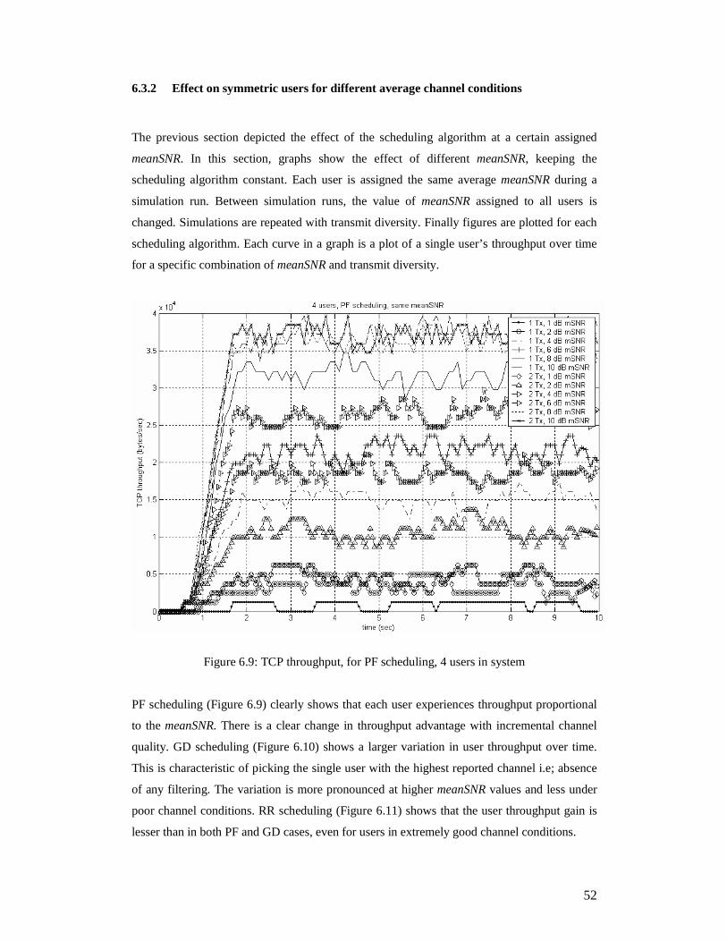
52

6.3.2 Effect on symmetric users for different average channel conditions

The previous section depicted the effect of the scheduling algorithm at a certain assigned

meanSNR. In this section, graphs show the effect of different meanSNR, keeping the

scheduling algorithm constant. Each user is assigned the same average meanSNR during a

simulation run. Between simulation runs, the value of meanSNR assigned to all users is

changed. Simulations are repeated with transmit diversity. Finally figures are plotted for each

scheduling algorithm. Each curve in a graph is a plot of a single user’s throughput over time

for a specific combination of meanSNR and transmit diversity.

Figure 6.9: TCP throughput, for PF scheduling, 4 users in system

PF scheduling (Figure 6.9) clearly shows that each user experiences throughput proportional

to the meanSNR. There is a clear change in throughput advantage with incremental channel

quality. GD scheduling (Figure 6.10) shows a larger variation in user throughput over time.

This is characteristic of picking the single user with the highest reported channel i.e; absence

of any filtering. The variation is more pronounced at higher meanSNR values and less under

poor channel conditions. RR scheduling (Figure 6.11) shows that the user throughput gain is

lesser than in both PF and GD cases, even for users in extremely good channel conditions.

53

Figure 6.10: TCP throughput, for GD scheduling, 4 users in system

Figure 6.12 brings the thoughts together. It depicts the joint effect of scheduling, transmit

diversity and channel conditions in terms of total downlink bytes. This graph picks 2 channel

conditions: meanSNR = 10 dB (good average power conditions), and meanSNR = 4 dB

(mediocre average power conditions). This figure gives a snapshot of the combined effect of

the three degrees of freedom: Diversity, scheduling and channel quality. As can be seen, at

very high SNRs, transmit diversity hurts capacity with PF and GD scheduling. On an

individual basis, GD scheduling always does better than PF scheduling.

PF scheduling is beneficial to the real world implementation at the BTS in terms of lower

buffer overhead requirements. Assuming that all users are given the same meanSNR, PF

scheduling ensures that each of the users get an equal share of the air interface and variation

in throughput is minimal between users. GD schedulers pick the best user; hence the

smoothing effect seen with PF is no longer seen with GD. In general, GD schedulers need

larger buffers and dynamic buffer control in the presence of sudden downlink BER spikes that

could happen due to instantaneous shadowing.

54

Figure 6.11: TCP throughput, RR scheduling, 4 users.

Total # bytes served by BTS in a 4 - user system for various scheduling algorithms

534310

222642

526153

648182

425200

632022

13299001295329

984040

130189212659841226880

0

200000

400000

600000

800000

1000000

1200000

1400000

1 1.2 1.4 1.6 1.8 2 2.2 2.4 2.6 2.8 3

Scheduler Type

To

tal b

ytes

4dB, 1 Tx 4dB, 2 Tx 10dB, 1 Tx 10dB, 2 Tx

RR PF GD

Low SNR regime

High SNR regime

Figure 6.12: Total downlink bytes to 4 users for various schedulers, diversity and channels.

55

Inferences:

1. If all users are assigned the same average channel condition, there is a reasonable

advantage in picking the best users i.e; using GD scheduling. The users receive

approximately the same number of slots since they see approximately the same

channel and hence have nearly the same likelihood of decoding a packet.

2. GD scheduling always does a little better than PF scheduling for all channel

conditions and for all diversity conditions; this is a characteristic of picking the best

user every slot period.

3. In a lightly loaded system with a similar distribution of users, when all users are in

good channel conditions, there is loss in capacity with transmit diversity, irrespective

of scheduling algorithm. This is obviously because of transmit diversity equalizing

the available user diversity and due to the saturation effect in good channels.

4. Transmit diversity has substantial benefits for users in weak channels, since it helps

these users see better channels and receive a higher number of slots.

5. PF schedulers ensure lower peak-to-trough variation in user throughput, thus reducing

the complexity in buffer implementation at the BTS.

6. Hence, it is still better to use PF scheduling due to 1) the relative invariance in

throughput trend for if all users are in poor channels and 2) No significant reduction

in throughput compared to GD scheduling.

6.4 The effects of user loading via 10 asymmetric system users

This section deals with the effect of asymmetric users. Each user is assigned a different

meanSNR.. For simulation purposes, the users are numbered from 1 to 10 and are assigned

meanSNR as in Table 6.1. The assignment of users to meanSNR is similar to keeping user 1

through 10 progressively nearer the BTS, i.e; users 1, 2 are somewhere near the edge of the

cell, while user 10 is near the cell site.

6.4.1 Joint effect of scheduling and transmit diversity on asymmetric users.

Figures 6.13, 6.14 and 6.15 depict the mean RLP throughput for each user for each scheduling

algorithm. Each curve in the graph depicts user throughput with and without transmit

diversity. Instead of plotting the user throughput over time as was done in the previous

sections (this can be complicated with 10 users), we compute and plot the average user

throughput.

56

User Number meanSNR assigned to user (dB)

1 3.0

2 3.0

3 4.0

4 4.0

5 5.0

6 6.0

7 7.0

8 8.0

9 9.0

10 10.0

Table 6.1: meanSNR assigned to users

In Figure 6.13, we see the clear advantage of using transmit diversity if RR scheduling is

used. Transmit diversity has a clear advantage for all user channel conditions. However, the

gain of transmit diversity decreases as percentage of throughput (implicitly, channel quality).

In Figure 6.14, GD scheduling is used. Users in bad channels are never scheduled. The extent

to which poor users starve is clearly indicated. Even users with average SNR see poor

throughput, since there is always a better user available to be scheduled. Hence, there is no

gain for poor users with Tx-diversity and GD scheduling, since they simply do not have

chance to be scheduled while there are other users in the system that experience far better

channel conditions. In Figure 6.15, PF scheduling is used. The advantage of using 2 transmit

antennas with PF scheduling is not as much as using 2 transmit antennas with RR scheduling.

This is implicit if one compares Figure 6.13 and Figure 6.15.

57

Average RLP throughput for each user in a 10 users/sector in system, RR scheduling

0

20000

40000

60000

80000

100000

120000

0 1 2 3 4 5 6 7 8 9 10

User #

Th

rou

gh

pu

t (b

ps)

1 Tx Antenna, RR Scheduling 2 Tx Antenna, RR Scheduling

Figure 6.13: Mean throughput for each of 10 users, RR scheduling.

Average RLP throughput for each user in a 10 users/sector in system, Greedy scheduling

0

100000

200000

300000

400000

500000

600000

700000

0 1 2 3 4 5 6 7 8 9 10

User #

Th

rou

gh

pu

t (b

ps)

1 Tx Antenna, Greedy Scheduling 2 Tx Antenna, Greedy Scheduling

Figure 6.14: Mean throughput for each of 10 users, GD scheduling.

58

Average RLP throughput for each user in a 10 users/sector in system, PF scheduling

0

20000

40000

60000

80000

100000

120000

140000

160000

180000

200000

0 1 2 3 4 5 6 7 8 9 10

User #

Th

rou

gh

pu

t (b

ps)

1 Tx Antenna, PF Scheduling 2 Tx Antenna, PF Scheduling

Figure 6.15: Mean throughput for each of 10 users, PF scheduling.

There are 2 interesting and paradoxical observations to be made between PF and GD

scheduling:

1. For PF scheduling, single transmit antenna systems are advantageous for users in high

channel conditions. Hence, transmit diversity actually hurts the users seeing very

good channels for a sufficiently long time. In Figure 6.14, pay attention to the

crossover region where the transmit diversity curve dips below non-transmit diversity

curve. For PF scheduling, user 8, 9 and user 10 are affected from transmit diversity.

From Table 6.1 there are users in reasonably good conditions (user 5, 6, 7) who could

report SNR comparable to that of 9 and 10. Transmit diversity tends to smooth out

both peaks and valleys of the fading channel for all users. In addition, transmit

diversity gain is more for users in bad channels. Hence, users in bad and medium

quality channels get scheduled more often (the number of slots are proportional to the

average channel seen), while users in good channels get scheduled less often (since

the ratio of average channel seen by these users to the other users is decreased).

Therefore, not only are slots being taken away by good quality users due to the nature

of the scheduler, but users in lower quality channels receive a larger proportion of

slots due to transmit diversity. As a result, transmit diversity hurts good channel users

with PF scheduling.

59

2. With GD scheduling, the trend is reversed. Bad and medium channel quality users

suffer due to transmit diversity, while users in a transmit diversity system and good

channel conditions see gain over non-transmit diversity good channel users. In 6.15,

notice the crossover region where the non-transmit diversity curve dips below the

transmit diversity curve. We know that GD scheduling selects a user based on the

highest instantaneous SNR reported by the 10 users. For GD scheduling, user 9 and

10 profit due to transmit diversity, while the poorer users suffer. Even though the

poor and mid-quality users may see SNRs that can support a higher order modulation

scheme compared to the same users without transmit diversity, the system is

constrained by a fixed number of slots. These slots are likely given to the top 2 users

in the system, hence transmit diversity helps the best users in a system with GD

scheduling. To summarize, in GD scheduling, at high SNR, the benefit of Tx-

diversity to the physical layer is far outweighed by the loss at the scheduler.

6.4.2 TCP trend for schedulers with transmit diversity for well distributed users

Figure 6.16 is significant because it compares the average TCP throughput for PF and RR

scheduling. The TCP throughput more or less follows the trend established at the RLP layer

for users in all channels. This graph reinforces the fairness advantage of using PF scheduling

for TCP, and the throughput gains associated with it.

Average TCP throughput for 10 users/sector in system, PF scheduling vs RR Scheduling

0

5000

10000

15000

20000

25000

0 1 2 3 4 5 6 7 8 9 10

User #

Th

rou

gh

pu

t (b

ytes

/sec

)

1 Tx Antennas, RR Scheduling 2 Tx Antennas, RR Scheduling 1 Tx Antennas, PF Scheduling 2 Tx Antennas, PF Scheduling

Figure 6.16: Mean TCP throughput comparison for 10 users, PF versus RR scheduling.

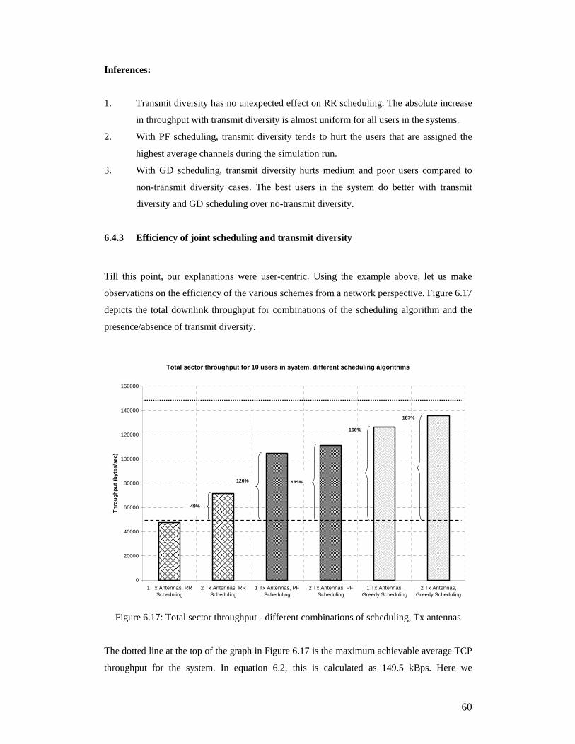
60

Inferences:

1. Transmit diversity has no unexpected effect on RR scheduling. The absolute increase

in throughput with transmit diversity is almost uniform for all users in the systems.

2. With PF scheduling, transmit diversity tends to hurt the users that are assigned the

highest average channels during the simulation run.

3. With GD scheduling, transmit diversity hurts medium and poor users compared to

non-transmit diversity cases. The best users in the system do better with transmit

diversity and GD scheduling over no-transmit diversity.

6.4.3 Efficiency of joint scheduling and transmit diversity

Till this point, our explanations were user-centric. Using the example above, let us make

observations on the efficiency of the various schemes from a network perspective. Figure 6.17

depicts the total downlink throughput for combinations of the scheduling algorithm and the

presence/absence of transmit diversity.

Total sector throughput for 10 users in system, different scheduling algorithms

0

20000

40000

60000

80000

100000

120000

140000

160000

1 Tx Antennas, RRScheduling

2 Tx Antennas, RRScheduling

1 Tx Antennas, PFScheduling

2 Tx Antennas, PFScheduling

1 Tx Antennas,Greedy Scheduling

2 Tx Antennas,Greedy Scheduling

Th

rou

gh

pu

t (b

ytes

/sec

)

49%

187%

166%

133% 120%

Figure 6.17: Total sector throughput - different combinations of scheduling, Tx antennas

The dotted line at the top of the graph in Figure 6.17 is the maximum achievable average TCP

throughput for the system. In equation 6.2, this is calculated as 149.5 kBps. Here we

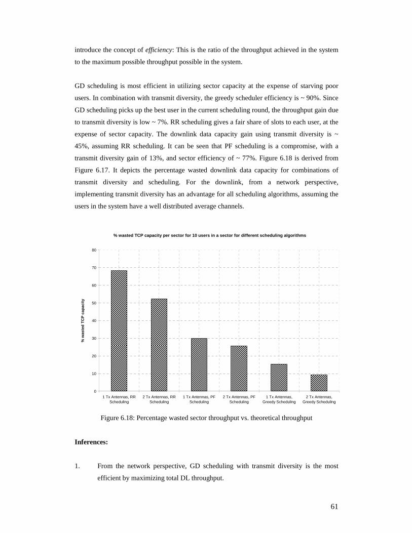
61

introduce the concept of efficiency: This is the ratio of the throughput achieved in the system

to the maximum possible throughput possible in the system.

GD scheduling is most efficient in utilizing sector capacity at the expense of starving poor

users. In combination with transmit diversity, the greedy scheduler efficiency is ~ 90%. Since

GD scheduling picks up the best user in the current scheduling round, the throughput gain due

to transmit diversity is low ~ 7%. RR scheduling gives a fair share of slots to each user, at the

expense of sector capacity. The downlink data capacity gain using transmit diversity is ~

45%, assuming RR scheduling. It can be seen that PF scheduling is a compromise, with a

transmit diversity gain of 13%, and sector efficiency of ~ 77%. Figure 6.18 is derived from

Figure 6.17. It depicts the percentage wasted downlink data capacity for combinations of

transmit diversity and scheduling. For the downlink, from a network perspective,

implementing transmit diversity has an advantage for all scheduling algorithms, assuming the

users in the system have a well distributed average channels.

% wasted TCP capacity per sector for 10 users in a sector for different scheduling algorithms

0

10

20

30

40

50

60

70

80

1 Tx Antennas, RRScheduling

2 Tx Antennas, RRScheduling

1 Tx Antennas, PFScheduling

2 Tx Antennas, PFScheduling

1 Tx Antennas,Greedy Scheduling

2 Tx Antennas,Greedy Scheduling

% w

aste

d T

CP

cap

acit

y

Figure 6.18: Percentage wasted sector throughput vs. theoretical throughput

Inferences:

1. From the network perspective, GD scheduling with transmit diversity is the most

efficient by maximizing total DL throughput.

62

2. With respect to the network, transmit diversity is beneficial for all scheduling

schemes but most beneficial for RR scheduling.

6.5 Histogram of slots/user for various schedulers.

In the next 3 graphs, the system is further loaded to 15 users, with each user performing full

rate FTP downloads. The intention is to show the distribution of slots per user when each is in

a different channel condition. This section is included to depict the general trend for the

number of slots/user for different scheduling algorithms. Each user is assigned a different

meanSNR. The meanSNR value assigned in this section is not as important as the trend. Users

from 1 to 15 are given monotonically increasing meanSNR in steps of 1dB. The only

exception is that users 1 and 2 are given the same average channel quality. Users 3 and 4 are

also given the same, but a slightly higher average channel quality. As a result, the PF

scheduler assigns approximately the same number of slots to these users. This is shown in

Figure 6.19. Greedy scheduling in Figure 6.20 shows the clear bias towards users close to the

BTS. RR scheduling shown in Figure 6.21 shows the equal allocation of slots between all the

15 system users.

Histogram of scheduling slots for a 15 user system, proportionally fair scheduling

0

100

200

300

400

500

600

700

1 2 3 4 5 6 7 8 9 10 11 12 13 14 15

User

Figure 6.19: Histogram of slots assigned per user, proportionally fair scheduling

63

Histogram of scheduling slots for a 15 user system, Greedy scheduling

0

1000

2000

3000

4000

5000

6000

1 2 3 4 5 6 7 8 9 10 11 12 13 14 15

User

Figure 6.20: Histogram of slots assigned per user, greedy scheduling

Histogram of scheduling slots for a 15 user system, round robin scheduling

0

100

200

300

400

500

600

1 2 3 4 5 6 7 8 9 10 11 12 13 14 15

User

Figure 6.21: Histogram of slots assigned per user, Round robin scheduling

64

Inferences:

1. RR scheduling is not biased towards any user.

2. GD scheduling is biased towards the best systems users.

3. PF scheduling distributes slots proportional to the average channel seen by each user.

6.6 Effect of receive diversity

This section introduces receive diversity and the effect of joint transmit-receive diversity

channels on user throughput. We term simulations that use joint transmit and receive diversity

as MIMO system simulations. We use the term MIMO specifically in the context of MRC

combining on the multiple receive antenna elements with transmit diversity. This section

follows the trend established in previous sections: first, we consider a single user scenario,

then introduce the effect of scheduling via multiple users and finally examine the joint effect

of scheduling, MIMO and user diversity by assigning different channels to each user.

6.6.1 Receive diversity and MIMO gains for single user systems

Consider the single user scenario, where every downlink slot is available to the user. Figure

6.22 depicts user throughput under the 4 conditions –

1. 1 Tx, 1 Rx (SISO)

2. 2 Tx, 1 Rx (Transmit diversity alone)

3. 1 Tx, 2 Rx (Receive diversity alone)

4. 2 Tx, 2 Rx (MIMO)

65

RLP throughput, single user in system, mean Eb/No = 10 dB, various Tx-Rx antenna combinations

0

200000

400000

600000

800000

1000000

1200000

1400000

1600000

1800000

0 1 2 3 4 5 6 7 8 9 10

time (sec)

thro

ug

hp

ut

(bit

s/se

c)

1 Tx 1 Rx antenna 1 Tx 2 Rx antenna 2 Tx 1 Rx antenna 2 Tx 2 Rx antenna

Figure 6.22: Single user throughput – effect of receive diversity on throughput in bps

The user is assigned a very good average channel condition (10dB). In this section, we

assume that 64 QAM modulation scheme is available. In the case of MIMO, the user always

tends to report a channel capable of supporting the highest order modulation scheme and

hence sees the highest throughput.

Figure 6.23 depicts the average throughput increase seen by the user for 4 diversity situations.

The effect of receive diversity is more pronounced than the effect of transmit diversity due to

the power penalty associated with transmit diversity. There is a near doubling (80%) of user

throughput going from SISO to MIMO.

66

Average throughput gain for a single user system for different diversity types

0

200000

400000

600000

800000

1000000

1200000

1400000

1600000

1 Tx 1 Rx antenna 2 Tx 1 Rx antenna 1 Tx 2 Rx antenna 2 Tx 2 Rx antenna

Diversity type

Th

rou

gh

pu

t 27%

51%

80%

Figure 6.23: Average throughput increase for a single user with diversity.

6.6.2 Gains using MIMO in a system with 10 symmetric users

Now, let’s load the system with 10 users. Initially, the same meanSNR is assigned to all the 10

users (10 dB). This has the effect of users arranged in a concentric circle around the BTS. The

reason for the study is to normalize the effect of channel quality, and concentrate largely on

the effect of MIMO and scheduling. Figure 6.24 depicts the effect of GD scheduling and

different transmit-receive combinations for the 10 users in the system. The graph shows that

when GD scheduling is implemented, if the mobile device implements receive diversity, users

do not experience much gain with transmit diversity. This is likely due to GD scheduling

picking the best user, and since the users are placed in good channels, the chosen user is

always likely scheduled with the maximum modulation order, resulting in saturation.

Transmit diversity-alone has some gain over SISO, as expected. Even though the users are in

the same average channel condition, there is some variation in throughput from user to user.

This can be attributed to the effect of GD scheduling picking the instantaneous good channel

user and to the statistical effect of user diversity.

Figure 6.25 depicts the effect of PF scheduling. The graph clearly depicts how the fairness

criteria for the PF scheduler smoothes out the throughput variation seen by each user in GD

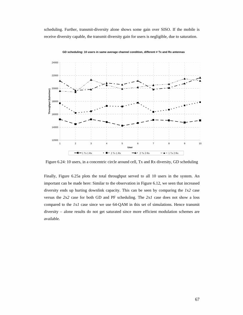
67

scheduling. Further, transmit-diversity alone shows some gain over SISO. If the mobile is

receive diversity capable, the transmit diversity gain for users is negligible, due to saturation.

GD scheduling: 10 users in same average channel condition, different # Tx and Rx antennas

12000

14000

16000

18000

20000

22000

24000

1 2 3 4 5 6 7 8 9 10

User

Th

rou

gh

pu

t (b

ytes

/sec

)

1 Tx 1 Rx 2 Tx 1 Rx 2 Tx 2 Rx 1 Tx 2 Rx

Figure 6.24: 10 users, in a concentric circle around cell, Tx and Rx diversity, GD scheduling

Finally, Figure 6.25a plots the total throughput served to all 10 users in the system. An

important can be made here: Similar to the observation in Figure 6.12, we seen that increased

diversity ends up hurting downlink capacity. This can be seen by comparing the 1x2 case

versus the 2x2 case for both GD and PF scheduling. The 2x1 case does not show a loss

compared to the 1x1 case since we use 64-QAM in this set of simulations. Hence transmit

diversity – alone results do not get saturated since more efficient modulation schemes are

available.

68

PF scheduling: 10 users in same average channel condition, different # Tx and Rx antennas

14000

15000

16000

17000

18000

19000

20000

21000

1 2 3 4 5 6 7 8 9 10

User

Th

rou

gh

pu

t (b

ytes

/sec

)

2 Tx 2 Rx 2 Tx 1 Rx 1 Tx 1 Rx 1 Tx 2 Rx

Figure 6.25: 10 users, in a concentric circle around cell, Tx and Rx diversity, PF scheduling

Total average throughput for 10 system users

170872

209236 206506.6667

148304

169301.3333

206890.6667 205592

1

148469.3333

0

50000

100000

150000

200000

250000

1x1+ GD 2x1 + GD 1x2 + GD 2x2 + GD 1x1+ PF 2x1 + PF 1x2+ PF 2x2 + PF

Scheduler and diversity combination

Th

rou

gh

pu

t (b

ytes

/sec

)

Tx Diversity hurts ...

Figure 6.25a: Total throughput served for different scheduler and diversity combinations

69

Inferences:

1. Assuming that users are assigned similar meanSNR, GD scheduling does better than

PF scheduling for both receive diversity and MIMO cases. The inferences of section

6.3 can be applied to explain the effect of receive diversity and 2x2 cases.

2. Under the same situation, there is negligible gain with transmit diversity for any

scheduling algorithm, if the mobile is receive-diversity capable. On the contrary,

adding more diversity (in this case, transmit diversity) to a system nearing saturation

ends up hurting system capacity, irrespective of scheduler type.

6.6.3 Gains using MIMO in a 10-user system with asymmetric/well-distributed users

In the next scenario, each user is assigned meanSNR as in Table 6.1, to study a more realistic

distribution of users. Figure 6.26 depicts the effect of RR scheduling on each user.

RR scheduling: 10 users in different RF condition, different # Tx and Rx antennas

0

2000

4000

6000

8000

10000

12000

14000

16000

18000

20000

1 2 3 4 5 6 7 8 9 10

Users

2 Tx 1 Rx 2 Tx 2 Rx 1 Tx 2 Rx 1 Tx 1 Rx

Figure 6.26: 10 users, at different points in the cell, Tx and Rx diversity, RR scheduling

For RR scheduling, there is a constant increase in throughput for every user going from SISO

to MIMO. The scheduling algorithm does not interfere with the user throughput. Figure 6.27

shows the effect of GD scheduling, and Figure 6.28 zooms into the area of interest. Figure

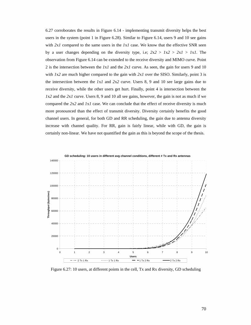
70

6.27 corroborates the results in Figure 6.14 - implementing transmit diversity helps the best

users in the system (point 1 in Figure 6.28). Similar to Figure 6.14, users 9 and 10 see gains

with 2x1 compared to the same users in the 1x1 case. We know that the effective SNR seen

by a user changes depending on the diversity type, i.e; 2x2 > 1x2 > 2x1 > 1x1. The

observation from Figure 6.14 can be extended to the receive diversity and MIMO curve. Point

2 is the intersection between the 1x1 and the 2x1 curve. As seen, the gain for users 9 and 10

with 1x2 are much higher compared to the gain with 2x1 over the SISO. Similarly, point 3 is

the intersection between the 1x1 and 2x2 curve. Users 8, 9 and 10 see large gains due to

receive diversity, while the other users get hurt. Finally, point 4 is intersection between the

1x2 and the 2x1 curve. Users 8, 9 and 10 all see gains, however, the gain is not as much if we

compared the 2x2 and 1x1 case. We can conclude that the effect of receive diversity is much

more pronounced than the effect of transmit diversity. Diversity certainly benefits the good

channel users. In general, for both GD and RR scheduling, the gain due to antenna diversity

increase with channel quality. For RR, gain is fairly linear, while with GD, the gain is

certainly non-linear. We have not quantified the gain as this is beyond the scope of the thesis.

GD scheduling: 10 users in different avg channel conditions, different # Tx and Rx antennas

0

20000

40000

60000

80000

100000

120000

140000

0 1 2 3 4 5 6 7 8 9 10

Users

Th

rou

gh

pu

t (b

ytes

/sec

)

2 Tx 1 Rx 1 Tx 1 Rx 1 Tx 2 Rx 2 Tx 2 Rx

Figure 6.27: 10 users, at different points in the cell, Tx and Rx diversity, GD scheduling

71

Figure 6.28: Zoomed in view for Figure 6.27

Figure 6.29 depicts PF scheduling. With PF scheduling, transmit-diversity gain over SISO is

lesser compared to receive-diversity gain over SISO. Again, transmit-diversity-alone hurts

good channel users. With PF scheduling, implementing simple receive-diversity results in

large gain over SISO or transmit-diversity-alone for all users. An interesting trend is seen if

we compare the 1x2 case and the 2x2 case. At very high SNR (User 10), we see again that

transmit diversity hurts the users with the best channels. For the range of simulated

meanSNRs (1 dB to 10 dB), receive-diversity-alone does hurt the very good channel users (as

was seen with the best users in the system for transmit-diversity-alone simulations, Figure

6.14 and Figure 6.15), but the trend suggests that had the simulation been performed for

increasing meanSNR, a point would be reached where receive diversity would start to hurt the

best users. It is plausible to conclude that users in excellent channels are bound to suffer when

implementing transmit or receive diversity compared to the no-diversity case if they remain

stationary and their channel quality remains sufficiently high.

Finally, Figure 6.29a brings together the observations from the network perspective, similar to

the study in Figure 6.17. To put the results in perspective, the figure depicts the % increase in

throughput going through various combinations of scheduling algorithms and diversity

conditions.

72

PF scheduling: 10 users in diff. avg. channel condition, diff. # Tx and Rx antennas

0

5000

10000

15000

20000

25000

30000

1 2 3 4 5 6 7 8 9 10Users

Th

rou

gh

pu

t (b

ytes

/sex

)

1 Tx 1 Rx 1 Tx 2 Rx 2 Tx 2 Rx 2 Tx 1 Rx

Figure 6.29: 10 users, at different points in the cell, Tx and Rx diversity, PF scheduling

Total sector throughput for 10 systems users, different scheduling algorithms and diversity combinations

0

20000

40000

60000

80000

100000

120000

140000

160000

180000

200000

1Tx-1Rx,RR

2Tx-1Rx,RR

1Tx-2Rx,RR

2Tx-2Rx,RR

1Tx-1Rx,PF

2Tx-1Rx,PF

1Tx-2Rx,PF

2Tx-2Rx,PF

1Tx-1Rx,GD

2Tx-1Rx,GD

1Tx-2Rx,GD

2Tx-2Rx,GD

Scheduler/diversity combination

Th

rou

gh

pu

t (b

ytes

/sec

)

48%

101%

151% 114%

132%

186%

234%

170%

189%

251%

315%

Figure 6.29a: Total sector throughput - different combinations of scheduling algorithms and

diversity conditions.

73

6.7 The effect of motion on antenna diversity and user diversity

The results till this point assumed that the users in the system were in stationary to low

motion environments (we used a Doppler shift = 5 Hz to generate the Rayleigh fade variables)

and the mean channel quality was fixed throughout the simulation run. In reality, the system

will consist of users in various motion scenarios – some stationary, some pedestrian and some

in a high speed auto. This section deals with the statistical effect of user motion combined

with antenna and user diversity. In this section, we simulate the effect of user motion from

and away from the cell site. The meanSNR of each user varies as the simulation run

progresses. This simulates the effect of high speed motion and shadowing.

6.7.1 “SameRF” simulations

The first sets of simulations are called “Same RF” simulations. The “Same RF” notation

indicates that all 10 users are assigned the same meanSNR, and this meanSNR is changed

during the simulation run. All users move away or towards the BTS simultaneously (e.g;

users in a bus). Another way of picturing this is by keeping the users spaced equally in a

radial fashion around the BTS. The users are then moved radially outwards towards the cell

boundary or inwards towards the cell center.

Let’s begin with Figure 6.30 - an example of the SameRF notation. This is a plot of the total

bytes received by each user. The figure contrasts the effect of using GD versus PF scheduling

in SISO (1x1) versus MIMO (2x2) conditions. With SISO, the total bytes per user in a 10

second simulation run is approximately 375 Kbytes. The total bytes received for each user in

the MIMO case is approximately 4 times that of SISO, around 1400 Kbytes.

In SameRF simulations, there is no significant advantage in using PF over GD scheduling,

and this is intuitive. Figure 6.31a and Figure 6.31b zoom into the trends seen in Figure 6.30

for each of the diversity conditions. The point to take away from these graphs is the peak-to-

trough variation in user throughput for each scheduling scheme. Irrespective of the diversity

situation, GD scheduling seems to have a large variation in throughput, while the PF always

follows a smoother curve.

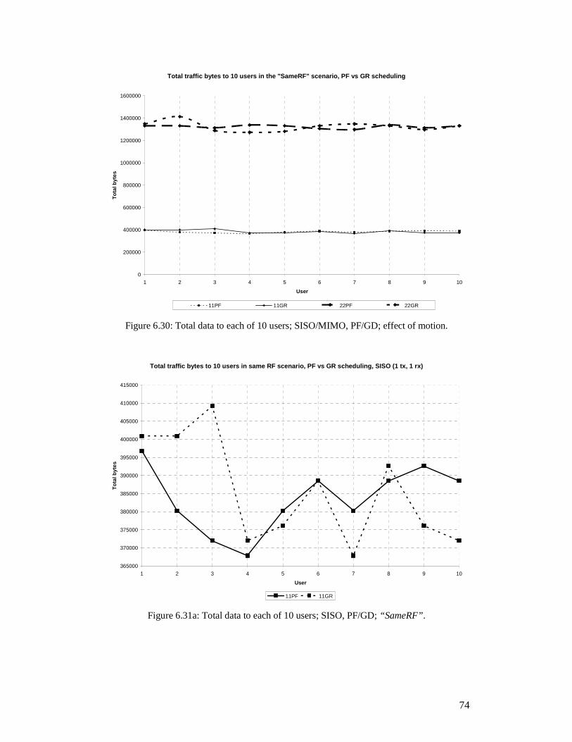
74

Total traffic bytes to 10 users in the "SameRF" scenario, PF vs GR scheduling

0

200000

400000

600000

800000

1000000

1200000

1400000

1600000

1 2 3 4 5 6 7 8 9 10

User

To

tal b

ytes

11PF 11GR 22PF 22GR

Figure 6.30: Total data to each of 10 users; SISO/MIMO, PF/GD; effect of motion.

Total traffic bytes to 10 users in same RF scenario, PF vs GR scheduling, SISO (1 tx, 1 rx)

365000

370000

375000

380000

385000

390000

395000

400000

405000

410000

415000

1 2 3 4 5 6 7 8 9 10

User

To

tal b

ytes

11PF 11GR

Figure 6.31a: Total data to each of 10 users; SISO, PF/GD; “SameRF”.

75

Total traffic bytes to 10 users in same RF scenario, PF vs GR scheduling, MIMO (2 tx, 2 rx)

1260000

1280000

1300000

1320000

1340000

1360000

1380000

1400000

1420000

1440000

1 2 3 4 5 6 7 8 9 10

User

To

tal b

ytes

22PF 22GR

Figure 6.31b: Total data to each of 10 users; MIMO, PF/GD; “SameRF”.

Inferences:

1. With SameRF simulations (rapid changes in meanSNR for all users), there is not

much to be gained by using PF over GD. Again, in terms of total number of bytes

sent to the user over the simulation run, GD scheduling outscores PF scheduling.

2. In a loaded system, the total data sent to all users with MIMO is ~ 4x times the

amount of data sent to users in a SISO system.

6.7.2 “Different RF” simulations

The next sets of simulations are called “Different RF” simulations. The “Different RF”

notation randomizes motion for each of the 10 users. Initially, the 10 users are allocated

meanSNR as per Table 6.1. Every second thereafter, the meanSNR for each user is

incremented by 1 dB. This means these users are moving towards the base station. This gives

the chance for users in poor initial conditions to make up for lost data throughput. Then, users

with meanSNR > 7dB are transitioned to 4 dB. This is an example of sudden shadowing.

Since meanSNR is continuously incremented by 1dB every second, these users eventually

emerge from the shadow zone and regain good coverage. Thus, users in excellent initial

condition see bad channels later in the run.

76

As an example, user 4 is initially assigned meanSNR = 4 dB. At t=1, meanSNR = 5 dB, at t=3,

meanSNR = 7 dB. At the next decision period user 4 is downgraded to 4dB. The meanSNR

variation for each user is seen in Figure 6.32.

Variation in meanSNR trend for Users 1-10

0

1

2

3

4

5

6

7

8

9

1 2 3 4 5 6 7 8 9 10

Time (sec)

mea

nS

NR

(d

B)

User 1, 2 User 3, 4 User 5 User 6 User 7,8,9,10

Figure 6.32: Variation in meanSNR trend for each user in the “DifferentRF” simulation

As the simulation progresses, all users converge to the average channel region between 4dB

and 7dB. This region was chosen since we have seen from previous simulation results that it

is the region of maximum variation and sensitivity to the 3 degrees of freedom. Channel

quality is an indication of the total data received by each user, and this helps us study the

effect of the scheduling algorithm on system capacity. The average throughput for each user

will vary over time due to the varied assignment of meanSNR. We use total received bytes

over the duration of the simulation as a comparison statistic. Figure 6.33 depicts the effect of

the SISO channel with PF and GD scheduling. Figure 6.34 shows the effect if the MIMO

channel with PF, GD and RR scheduling.

77

Total traffic bytes to 10 users in diferent RF conditions, PF vs GR, SISO

0

100000

200000

300000

400000

500000

600000

1 2 3 4 5 6 7 8 9 10

User

Tra

ffic

to

eac

h u

ser

in b

ytes

PF Greedy

Figure 6.33: Total data to each of 10 users; SISO, PF/GD; “DifferentRF”.

Total traffic bytes to 10 users in diferent RF conditions, PF vs GR vs RR, MIMO

0

200000

400000

600000

800000

1000000

1200000

1 2 3 4 5 6 7 8 9 10

User

Tra

ffic

to

eac

h u

ser

in b

ytes

PF Greedy RR

Figure 6.34: Total data to each of 10 users; MIMO, PF/GD/RR; DifferentRF”.

In either case, the effect of user motion is normalized by PF scheduling. GD scheduling

shows large swings in user throughput, however, over time, the total data bytes sent by the

78

BTS with GD scheduling is always greater than the total number of bytes sent using PF

scheduling.

6.7.3 Scheduling and diversity effect on users with randomized motion

Figure 6.35 plots the total bytes sent from the BTS on the downlink for each of the following

conditions –

Case 1: SISO and GD

Case 2: SISO and PF

Case 3: MIMO and RR

Case 4: MIMO and PF

Case 5: MIMO and GD

This figure shows the advantage that GD scheduling has over PF scheduling for both diversity

conditions. With SISO, GD scheduling does marginally better than PF, around 4%. With

MIMO, GD scheduling allows the BTS to send around 9% more data on the downlink.

Total sector capacity over simulation run, MIMO vs SISO, users in sequential RF condition

0

1000000

2000000

3000000

4000000

5000000

6000000

7000000

8000000

1 2 3 4 5

Scheduling algorithm and diversity combination

To

tal b

ytes

fro

m t

he

sect

or

PF, 1x1 GD, 1x1 RR, 2x2 PF, 2x2 GD, 2x2

Figure 6.35: Total data bytes to 10 users, under rapid meanSNR variation

79

Inferences:

1. Irrespective of diversity, sector capacity due to GD scheduling is always greater than

with PF scheduling.

2. With respect to user experience, GD scheduling shows higher variation in data

delivery as compared to PF scheduling. This assumes that users are pseudo-randomly

moved around in the channel.

6.8 Tomlinson-Harashima Precoding and multi-user scheduling

The background theory for Tomlinson Harashima pre-coding is described in section 2.7 and

the implementation specifics are in section 5.11.

6.8.1 Reference simulations to baseline multi-user scheduling

For a theoretical evaluation, consider RR scheduling, since it guarantees a fixed number of

slots to a user in a given time interval. For multi-user scheduling cases, we assume 4 Tx

antennas, hence a maximum of 4 users can scheduled per time instant. Per second, there are

600 scheduling instants. Therefore, per second, effectively, 600 x 4 = 2400 users are

scheduled. These scheduling instants are divided equally (due to RR scheduling) between 10

users, hence in each second, 240 slots are assigned to each user, irrespective of channel

quality.

Let’s now assume that the total available transmit SNR is 20 dB. For a conservative estimate,

assume that during each scheduling instant, we use the most robust modulation scheme -

QPSK. As per Table 5.1, the assigned RLP segment size is 1024 bits.

Therefore, in the ideal case, throughput =

1024 x 240 = 245.76 kbps = 30.720 kBps. (6.4)

From Figure 6.36 it is seen that the simulation generates values that are consistent with

theoretical calculations.

80

THP scheduling: TCP throughput for RR scheduling, 20 dB transmit SNR

0

5000

10000

15000

20000

25000

30000

35000

0 2 4 6 8 10 12 14 16 18

time (sec)

thro

ug

hp

ut

(byt

es/s

ec)

Real-world channel conditions Perfect channel conditions (0% OTA erasure)

1024 x 240 = 30.720 kBps

Figure 6.36: THP: Ideal vs. real condition user throughput, RR, 20 dB transmit SNR

To generate the theoretical curve, we allow the user to be scheduled and always assume that

the packet to the user will be decoded correctly. This is unrealistic. Figure 6.36 depicts a

second curve in which users are scheduled based on the outputs of the scheduling pattern

generated for a particular sector power and scheduling scheme, but guaranteed delivery over

the air interface is not assumed. The packet might be lost due to inadequate power availability

and the RLP algorithm recovers these lost packets via retransmissions. This erasure and

retransmission mechanism causes the reduction in throughput. In Figure 6.36, throughput is

plotted for one among 10 users. The total downlink transmit SNR is 20 dB. RR scheduling is

used. Per simulation, throughput achieved for the user is ~ 23 kBps = 204 kbps.

Contrast equation 6.4 (multi-user scheduling) with the case of a single user scheduled every

scheduling instant. To compare apples with apples, load the system with the same number of

users. With 10 users in the system, 60 slots are assigned to the user per second. The difference

now is that the entire cell power is assigned to the same user. As a result, a more efficient

modulation scheme can be used (64-QAM or 16-QAM).

Assuming 4 transmit antenna elements and assuming that the SNR seen by each user is high

enough to use 16-QAM in every slot, the theoretical user throughput is-

2048 x 60 = 122.88 Kbps = 15.36 KBps (6.5)

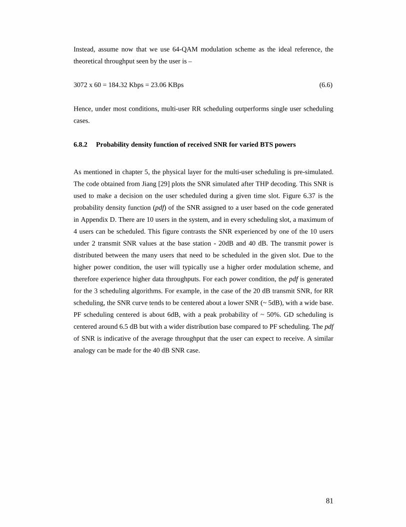
81

Instead, assume now that we use 64-QAM modulation scheme as the ideal reference, the

theoretical throughput seen by the user is –

3072 x 60 = 184.32 Kbps = 23.06 KBps (6.6)

Hence, under most conditions, multi-user RR scheduling outperforms single user scheduling

cases.

6.8.2 Probability density function of received SNR for varied BTS powers

As mentioned in chapter 5, the physical layer for the multi-user scheduling is pre-simulated.

The code obtained from Jiang [29] plots the SNR simulated after THP decoding. This SNR is

used to make a decision on the user scheduled during a given time slot. Figure 6.37 is the

probability density function (pdf) of the SNR assigned to a user based on the code generated

in Appendix D. There are 10 users in the system, and in every scheduling slot, a maximum of

4 users can be scheduled. This figure contrasts the SNR experienced by one of the 10 users

under 2 transmit SNR values at the base station - 20dB and 40 dB. The transmit power is

distributed between the many users that need to be scheduled in the given slot. Due to the

higher power condition, the user will typically use a higher order modulation scheme, and

therefore experience higher data throughputs. For each power condition, the pdf is generated

for the 3 scheduling algorithms. For example, in the case of the 20 dB transmit SNR, for RR

scheduling, the SNR curve tends to be centered about a lower SNR (~ 5dB), with a wide base.

PF scheduling centered is about 6dB, with a peak probability of ~ 50%. GD scheduling is

centered around 6.5 dB but with a wider distribution base compared to PF scheduling. The pdf

of SNR is indicative of the average throughput that the user can expect to receive. A similar

analogy can be made for the 40 dB SNR case.

82

THP scheduling: PDF of SNR assigned to one user among 10, different scheduling situations

0

0.05

0.1

0.15

0.2

0.25

0.3

0.35

0.4

0.45

0.5

0 2 4 6 8 10 12 14 16SNR (dB)

40 dB, PF 40 dB, GD 40 dB, RR 20 dB, PF 20 dB, GD 20 dB, RR

Figure 6.37: THP: PDF of SNR seen by a user, RR/PF/GD scheduling, 20/40 dB Tx-SNR.

6.8.3 Multi-user scheduling throughput/user with varied schedulers and BTS power.

Figure 6.38 depicts the results for an end-to-end simulation of multi-user scheduling. It

depicts the effect of 3 distinct BTS transmit SNR (20, 30 and 40 dB) for the three scheduling

schemes. It shows the gradual progression of user throughput with total available base station

power. It also indicates the variation seen in user throughput under different schedulers. With

PF scheduling, throughput remains fairly constant throughout the simulation run. GD

scheduling shows a variation over time for the same user. RR scheduling provides the worst

throughput, as expected, even with multiple scheduled users per time slot. The graph shows

that multi-user scheduling more or less follows the trends established in earlier sections.

The big advantage of multi-user scheduling is that many more slots are now available to the

same number of users. Hence, especially in the SNR regime, multi-user scheduling will likely

see higher throughput gain for users compared to the single user scheduling case.

83

THP scheduling : TCP throughput for one among 10 users

0

10000

20000

30000

40000

50000

60000

70000

80000

90000

0 2 4 6 8 10 12 14 16 18 20

Time (sec)

TC

P T

hro

ug

hp

ut

(byt

es/s

ec)

40 dB, PF 30 dB, PF 30 dB, RR 30 dB, GD 40 dB, GD 40 dB, RR 20 dB, PF

20 dB, GD 20 dB, RR

20 dB

30 dB

40 dB

Figure 6.38: TCP throughput, 1 user, varying scheduling schemes and BTS SNR.

6.8.4 Average gains for in a multi-user scheduling environment for various schedulers

Figure 6.39 summarizes Figure 6.38. It shows the degradation of throughput with reduced

BTS power for different scheduling schemes. The curves in the system depict the throughput

for one of the users in the system. At high BTS powers, GD scheduling does noticeably better

than PF. At low BTS powers, GD scheduling does marginally better then PF. This is not a

new result. The gain with GD scheduling over PF and RR scheduling reduces with reducing

BTS powers. Reducing the total BTS power is tantamount to allocating a lesser power to be

shared between the various users during each scheduling instant. This is consistent with

previous results in Figures 6.9 to 6.12. This graph also compares multi-user scheduling with

the 2x2 single-user scheduling case. The single-user scheduling case in this graph involves

associating each user with the same meanSNR (10 dB) in a 10-user system. The graph depicts

the difference in throughput going from the single-user case to multi-user scheduling for

various BTS power conditions. The results seem to point to the fact that multi-user scheduling

is universally always better than single-user scheduling - but is this really true?

It can be argued that the graph does not depict an apples-to-apples comparison. In the 2x2,

single-user scheduling case, each user sees a 10 dB channel, hence the total average BTS

SNR available is also 10 dB. Therefore, in effect, we are comparing the 10 dB SNR in a 2x2

84

case with a 20 dB THP case! However, if 10 dB BTS transmit SNR is to be shared (say

equally) between 4 users, each user would see approximately a 2.5 – 3 dB channel. This poor

channel will ensure that the user is in outage most of the time. Hence, a more practical

comparison is the 20 dB BTS power, shared between a maximum of 4 users per slot. This

should give each user approximately 5 dB of channel SNR, sufficient to support at least

QPSK. Now assume that in the 2x2, single user scheduling case, 20 dB were assigned to

every user. This is like a true apples-to-apples comparison. However, intuitively, the result

would not be much different than the 10 dB case since each user in the 10 dB channel is

already at saturation, with a majority of slots being scheduled with 64-QAM. 64-QAM results

in 6 bits per symbol, or a 3-fold increase in bandwidth efficiency over QPSK. However,

scheduling 4 users per slot versus scheduling 1 user per slot is a 4-fold increase in theoretical

available downlink data transfer capability. Hence, the gain due to the availability of multiple

schedulable slots far outweighs the loss due to paucity of power when multiple users are

scheduled, for practical power condition scenarios. This is evidenced by the gain (18% for

GD, 17% for PF and 28% for RR) in multi-user scheduling over the 2x2 single-user

scheduling case seen with 20 dB power. It’s also reasonable to say that while this comparison

is not exactly accurate, it is a fair approximation to achievable gains with multi-user

scheduling. Of course, the increase in BTS power requirement would involve a slew of other

system changes (cell size issues, system capacity concerns, etc).

Average TCP throughput for each scheduling algorithm for multi-user and single-user scheduling

0

10000

20000

30000

40000

50000

60000

70000

1 2 3

Scheduling algorithm

Th

rou

gh

pu

t (b

ytes

/sec

)

40 dB Tx SNR 30 dB Tx SNR 20 dB Tx SNR 2x2

GD PF RR

35%

83 %

18%

31%

28%

93%

17%

82%

40%

Figure 6.39: Average TCP throughput for 1 user under various scheduling schemes

85

% increase in TCP throughput for different scheduling algorithms and single vs multi-user scheduling

0

50

100

150

200

250

1 2 3

% in

crea

se in

TC

P t

hro

ug

hp

ut

PF GD RR

2x2 single user scheduling versus multi-user scheduling

(20 dB)

2x2 single user scheduling versus multi-user scheduling

(30 dB)

2x2 single user scheduling versus multi-user scheduling

(40 dB)

Figure 6.40: Increase in throughput going from single user to multi user scheduling for

various power conditions.

Figure 6.40 shows the percentage increase in throughput between single-user scheduling

versus multi-user scheduling for various levels of transmit power. The graphs should be

interpreted as follows:

1. Each curve depicts a different scheduling algorithm.

2. Each point depicts the increase in throughput of multi-user scheduling in a specific

power condition over single user scheduling with 2 transmit and 2 receive antennas.

With increasing BTS SNR, GD scheduling shows increasing gains in terms of absolute

numbers over PF scheduling and RR scheduling.

Finally 6.41 shows the total downlink throughput served to all 10 users in the system. The

graph contrasts the 2x2 single-user scheduling scheme against the multi-user scheduling using

THP for the 3 transmit power conditions mentioned above. This graph gives a one shot

summary for all the results described in this section.

86

Total downlink throughput served by the BTS for 10 users

0

100000

200000

300000

400000

500000

600000

700000

1 2 3 4 5 6 7 8 9 10 11 12

Th

rou

gh

pu

t (b

ytes

/sec

)

2 x2, single user scheduling 20 dB BTS Tx SNR 30 dB BTS Tx SNR 40 dB BTS Tx SNR

RR PF

RR PF

RR PF

RR PF

Figure 6.41: Total downlink throughput for all users - single-user vs multi-user scheduling.

Inferences:

1. In a loaded system, the user experience with multi-user scheduling via THP is better

than single user scheduling. This is due to the additional slots available to schedule

the user.

2. Assuming multi-user diversity, GD scheduling performs noticeably better than PF for

high BTS transmit power. For low BTS transmit SNR, the GD scheduling is

marginally better than PF scheduling.

3. In terms of absolute numbers, GD, PF and RR scheduling do increasingly better with

increasing BTS powers. Of course, eventually, throughput will saturate.

6.8.5 Thoughts on latency issues due to schedulers.

A point to be noted in all the scheduler graphs is the effect of latency. With RR scheduling,

the effect of latency is distributed across all users in the cell, i.e; data bytes to all users are

equally delayed. If the user is in a poor channel, the throughput is not reduced to the high

latency, but because the terminal is likely unable to decode the data at all.

87

With PF scheduling, latency is inversely proportional to the quality of the channel seen by the

user. Better the channel seen by the user, the more slots assigned, the higher the decoding

likelihood and hence lesser the latency. PF scheduling has the effect of shaping the latency

curve to the quality of the channel seen by the user.

With GD scheduling, the best users in a system are instantaneously scheduled. If the same

channel conditions are maintained for the user over a considerable period of time, the latency

will increase and be disastrous for poorer users in the same cell. The latency period is

dependent on channel conditions. In a real life scenario, users are expected to move around,

however, given a GD scheduler and given the real possibility that there might be a stationary

user under a cell site, the throughput for edge users will obviously decrease (due to the lack of

a scheduling slot) and latency will increase (thereby increasing the likelihood of TCP

retransmission). This effect is seen for the poorer users in the system with GD scheduling,

where the throughput for the user is effectively nil. Typical initial retransmission time out for

users is in the range of 3 seconds (this adaptively varies over the lifetime of the connection),

so, if traffic is initially sent and then the user travels into a low channel quality region, there is

a high likelihood of TCP retransmission due to high latency.

88

7. Conclusions

In this thesis, we simulated various scenarios to understand the interaction between

scheduling, various channel conditions and multiple antennas at the transmit and receive ends

of the communication chain. We started with a single user system, and showed that transmit

diversity is beneficial to the user for every channel condition. If the user constantly sees a

poor wireless channel, transmit diversity helps the user by almost tripling the experienced

throughput. We then loaded the system with 4 symmetric users, and assumed that every user

saw the same average channel. Under this assumption, we observe that GD and PF scheduling

perform nearly as well; this is expected, since the users statistically have an equal chance to

getting a downlink time slot. However, in terms of absolute numbers, GD scheduling always

performs better than PF, irrespective of diversity. GD scheduling ensures the highest total

downlink throughput from the BTS.

In the next step, we introduced significant amount of user diversity within the system by

simulating a 10 user system. In this set of simulations, each user is initially assigned a

different average channel, so as to magnify the deleterious effect of diversity with PF

scheduling. Given this situation, RR scheduling ensures that each user’s throughput increases

proportional to the channel quality, and transmit diversity in conjunction with RR scheduling

ensures a constant increase over SISO with RR. PF scheduling has the effect of hurting the

best users in the system if transmit diversity is used, however the poorer users in the system

benefit at the expense of slots given up by the best users. GD scheduling completely starves

the poor users. For the best channel users, GD scheduling with transmit diversity has an upper

hand over GD scheduling without transmit diversity. From a network perspective, GD always

performs better than any other scheduling scheme. GD scheduling with transmit diversity is

the most efficient among the schemes simulated. In our system, we observed that the wasted

DL capacity in terms of TCP throughput is under 10%.

We then introduced receive diversity within the simulation set and showed that in a single

user system, the throughput experienced by the user under MIMO (2 transmit, 2 receive

antennas) outperforms the throughput experienced under SISO conditions by ~ 80%. To

further extend the idea of receive diversity in a practical system, we simulated 10 users and

initially assigned each user the same average channel condition. Given this situation, we

observed that - if receive diversity is implemented, then transmit diversity has no significant

advantage on user experience for GD and PF scheduling. As a next step, we assigned a

89

different average channel condition to each user so as to enhance the influence of user

diversity. This was to check if implementing receive diversity has any effect on the trends

established with transmit diversity-alone cases. We observed that when receive diversity is

deployed, the general trend established for each user in the system, given the assigned channel

condition in the simulated environment is similar to the case of transmit-diversity-alone.

Finally, we simulated the effect of fluctuations in the average channel conditions. First, the

same average channel condition was assigned to each user and over the simulation run, the

channel condition was varied by the same value for every user. In this simulation, we saw that

the total byes sent to the users over the simulation run remains almost the same, irrespective

of whether GD or PF scheduling is used at the BTS. However, the number of bytes sent to

each user varies more in GD scheduling than in PF scheduling. This can be attributed

to the fact that GD scheduling uses instantaneous channel conditions to decide on the

scheduled user. In a second set, different average channel conditions were assigned to each

user, and the channels were varied for each user over the simulation run. In this truly

randomized system, GD scheduling with MIMO maximizes the total sector capacity in terms

of the total number of bytes delivered by the system on the downlink. GD scheduling showed

~ 9% improvement over PF with MIMO, while GD performed 4% better than PF with SISO.

To complete our study, we explored multi-user scheduling based on the concepts developed

by Jiang [29]. We simulated a system where a maximum of 4 users can be scheduled out of

10 during a time slot. We simulated the throughput for 3 different BTS transmit powers and

concluded that GD scheduling in the multi-user scenario enhances user experience for high

BTS powers. GD scheduling performs as well as PF scheduling for low transmit powers. We

compared multi-user scheduling for various BTS powers to the case of single user scheduling

in a 10-user system environment where each user is assigned the same meanSNR. We

observed that multi-user scheduling outperforms single user scheduling for all simulated

conditions.

7.1 Future work

Typically, PF schedulers are used in commercial wireless systems. Scheduler design

is left to the infrastructure vendor so as to give room for competition, and specifications do

not mandate the use of one scheduler versus another. Several variants of PF scheduling have

been proposed in the literature [62, 63] and chapter 2 references sophisticated schedulers to

select between users. Some of these promising schedulers need to be studied from the user

90

perspective and especially so in the case of transmit and receive diversity. For example, the

authors in [62] propose a PF scheduler variant that is tuned to overcome the effect of inter-

scheduling intervals.

Another problem statement is - Given a scheduler that maximizes DL capacity (the focus of

several studies), is there one that also maximizes the gains for distributed users? Given a

specific spatial distribution of users and typical mobility ranges, what effect would the

proposed scheduler have on each user? If MIMO were implemented, would the scheduler

need to be modified?

Another proposal is that of hybrid scheduling: Given that different schedulers have different

effects on users in different channel ranges, one could optimize the system as follows –

a) Dividing users into groups, based on quantized instantaneous SNRs.

b) Use a different scheduling algorithm between users in each group

c) Use a proportionally fair scheduler between groups.

Would this scheduler still be fair to all system users? Would the scheduler be fair if MIMO

were used?

Multi-user scheduling: Although the commonly deployed 1xEVDO (Rev 0) specification

does not propose multi-user scheduling, the competitor standard in the UMTS world

(HSDPA) proposes mandatory support for this feature. In HSDPA, power is shared between

users in terms of a distribution of OVSF codes to each user. This thesis used Jiang’s work

[29] used precoding and an extended PF scheduler for multi-user scheduling. An important

area of study is one of optimized schedulers in a multi-user scheduled environment.

Finally, there is a need for many system specific studies, for example, the effect of

sudden channel outage on users. In this thesis, we saw that over the simulation interval, TCP

did not really play a detrimental role in user experience. Many of our simulations included

bringing the user out of outage conditions quickly, giving TCP sufficient time to recover,

instead of timing out. This was because we were more interested on the interaction between

MIMO, user diversity and channel quality, rather than corner cases. However, in time slot

scheduled systems, prolonged outage is very real during serving sector selection (1xEVDO),

or cell re-pointing (HSDPA), or during HSDPA-GPRS handovers. Implementing MIMO

may not even help in this case. In the near future, given that CDMA-TDMA hybrid schemes

will carry the bulk of wide area data traffic, these studies are essential.

91

Given the complexity of future wireless systems, cross layer design is still in a very nascent

stage. Each time a new physical layer is developed, every layer of the stack above it must

be tuned before systems become commercially viable. Cross layer is certainly challenging and

has great research potential for several years to come.

92

8. References

[1] CTIA wireless, www.wowcomm.com/research_statistics/index.cfm/AID/10030

[2] F.Alam, "Simulation of Third Generation CDMA Systems", Master's Thesis, January

1999.

[3] B.Turner,M.Orange,“3G Tutorial”

http://www.nmscommunications.com/file/3G_Tutorial.pdf

[4] CDMA Development Group, http://www.cdg.org/technology/3g.asp

[5] B.D.Woerner, "Multiple Antenna Systems, VT-ECE 6504", Lecture 1, Slide 2.

[6] MATLAB 7, www.mathworks.com

[7] Q.Bi, R.R.Brown, D.Cui, A.D.Gandhi, C.Y.Huang, and S.Vitebsky, “Performance of

1xEV-DO Third-Generation Wireless High-Speed Data Systems”, Bell Labs

Technical Journal 7(3), 97–107 (2003),

http://www.cdg.org/resources/white_papers/files/Perf_DO.pdf

[8] B.D.Woerner, "Multiple Antenna Systems, ECE 6504", Lecture 4, Slide 1.

[9] B.D.Woerner, "Multiple Antenna Systems, ECE 6504", Lecture 5, Slide 1.

[10] R.Gozali, B.D.Woerner, "Applying the Calderbank-Mazo algorithm to space-time

trellis coding", Proceedings of the IEEE, Southeastcon 2000, 7-9 April 2000,

Page(s):309 – 314.

[11] S.M.Alamouti, "A simple transmitter diversity scheme for wireless communications,"

IEEE Journal on Selected Areas in Communications, Volume 16, Issue 8, Oct. 1998,

Page(s):1451 – 1458.

[12] L. J.Cimini, Jr, N.R.Sollenberger, "OFDM with diversity and coding for high bit-rate

mobile data applications," Proceedings of the 3rd International Workshop on Mobile

Multimedia Communications, Sept. 1996, Page(s):1233 - 1243.

[13] N.Seshadri, J.H.Winters, "Two signaling schemes for improving the error

performance of frequency-division-duplex (FDD) transmission systems using

transmitter antenna diversity", Proceedings of the IEEE, 43rd Vehicular Technology

Conference, 18-20 May 1993, Page(s):508 - 511.

[14] V.Weerackody, "Diversity for direct-Sequence spread spectrum system using

multiple transmit antennas," Conference records of the IEEE International

Conference on Communications, 1993, Volume: 3, 23-26 May 1993, Page(s):1775 -

1779.

[15] V.Tarokh, H.Jafarkhani, A.R.Calderbank, "Space-time block coding for wireless

communications: performance results", IEEE Journal on Selected Areas in

Communications, Volume: 17 , Issue: 3 , March 1999, Page(s):451 - 460.

93

[16] A.Naguib, V.Tarokh, N.Seshadri, and A.R.Calderbank, “Space-time coding and

signal processing for high data rate wireless communications”, AT&T Labs –

Research tutorial, www.dia.unisa.it/isit2000/tutorials/spacetime.pdf

[17] S.Shakkottai, T.S.Rappaport and P.C.Karlsson, “Cross-layer Design for Wireless

Networks”, June 23, 2003, http://www.ece.utexas.edu/~shakkott/Pubs/cross-layer.pdf

[18] B.L.Hughes, “Differential space-time modulation,” IEEE Transactions on

Information Theory, Vol. 46, Nov. 2000, Page(s):2567 - 2578.

[19] G.Ganesan and P.Stoica, “Differential modulation using space-time block codes,”

Conference Record of the Thirty-Fourth Asilomar Conference on Signals, Systems

and Computers, 2001, Page(s):236 - 240.

[20] M.Tao and R.S.Cheng, “Differential space-time block codes,” Proceedings of the

Global Telecommunications Conference – GLOBECOM, Vol.2, 2001, Page(s):1098 -

1102.

[21] V.Tarokh and H.Jafarkhani, “A differential detection scheme for transmit diversity”,

IEEE Journal On Selected Areas in Communications,Vol.1 8, July 2000,

Page(s):1169 - 1174.

[22] V.Tarokh, N.Seshadri, A.R.Calderbank, "Space-time codes for high data rate wireless

communication: performance criterion and code construction", IEEE Transactions on

Information Theory, Volume: 44 , Issue: 2 , March 1998, Page(s):744 - 765.

[23] R.Peterson, R.Zeimer and D.Borth, “Introduction to spread spectrum systems”,

Prentice Hall Inc, 1995, Page 429, Equation 7-56.

[24] R.Peterson, R.Zeimer and D.Borth, “Introduction to spread spectrum systems”,

Prentice Hall Inc, 1995, Page 436, Table 7-3.

[25] Data Services options for wideband spread spectrum systems: Radio Link Protocol

Type 2. TIA/EIA/IS-707-A.2, February 1998.

[26] R. Wesel and J.M Cioffi, “Achievable Rates for Tomlinson–Harashima Precoding”,

IEEE Transactions on Information theory, Vol. 44, No. 2, March 1998, Page(s):824 -

831.

[27] The decision feedback equalizer, www.ee.ccu.edu.tw/~wl/wireless_class/Chapter1

Cellular Concepts.pdf

[28] P.M. Castro and L.Castedo, “Adaptive THP for wireless communication systems”,

Proceedings of the Baiona Workshop on Signal Processing in Communications,

November 2004.

[29] J. Jiang, “Downlink Throughput Optimization for Wireless Packet Data Networks”,

PhD Dissertation, July 2004.

[30] D.Tse, “Multiaccess Fading Channels – Part I: Polymatroid Structure, Optimal

resource allocation and Throughput capacities”, IEEE Transactions on Information

94

Theory, Vol 44, No 7, November 1998, Page(s):2796 - 2815.

[31] R.Pankaj, A.Jalali, and R.Padovani, “Data Throughput of a HDR high efficiency

Personal Wireless Communication System”, Proceedings of the IEEE Vehicular

Technology Conference 2000, Page(s):1854 - 1858.

[32] P.Bender, P.Black, M.Grob, R.Padovani, N.Sindhushayana, Andrew Viterbi,

“CDMA/HDR: A Bandwidth-Efficient High-Speed Wireless Data Service for

Nomadic Users”, IEEE Communications Magazine, July 2000, Page(s):70 - 77.

[33] R.C. Elliot and W.A. Krzymein, “Scheduling algorithms for the cdma2000 packet

data evolution”, IEEE 56th Vehicular Technology Conference, Vancouver, Canada,

September 2002, vol 1, pp 304-310.

[34] N.Joshi, S.Kadaba, S.Patel, G.Sundaram, “Downlink scheduling in CDMA data

networks”, Proceedings of the 6th annual international conference on Mobile

computing and networking, Boston, 2000, Page(s) 179 – 190.

[35] Q.Wu, E.Esteves , “The cdma2000 HDR packet data system”, Advances in 3G

Enhanced Technologies for Wireless Communications, Chapter 4, March 2002,

Editors: Jiangzhou Wang and Tung- Sang Ng.

[36] H. Inamura, G. Montenegro, R. Ludwig, A. Gurtov, F. Khafizov, “TCP over Second

(2.5G) and Third (3G) Generation Wireless Networks” RFC 3481,

http://ietf.org/rfc/rfc3481.txt

[37] Y.Yemini, “The Netbook: An eElectronic course on computer networks”,

http://www1.cs.columbia.edu/netbook

[38] V. Paxson, M. Allman, "RFC2988 - Computing TCP's Retransmission Timer",

http://ietf.org/rfc2988.txt

[39] P.Karn, C. Partridge, "Improving Round-Trip Time Estimates in Reliable

Transport Protocols", SIGCOMM 87.

[40] F.Khafizov, M.Yavuz, “TCP over cdma2000 networks”,

www.ietf.org/proceedings/01dec/slides/pilc-1.

[41] C.Liu, R.Jain, "Approaches of wireless TCP enhancement and a new proposal based

on congestion coherence", Proceedings of the 36th Annual Hawaii International

Conference on System Sciences 2003, 6-9 Jan. 2003, Page(s):10 - 14.

[42] A. Bakre, B.R. Badrinath, “I-TCP: indirect TCP for mobile hosts”, 15th International

Conference on Distributed Computing Systems (ICDCS'95), May 30 - June 02, 1995,

Page(s):136 - 143.

[43] T.S Rappaport; A. Annamalai; R.M. Buehrer; W.H Tranter,

“Wireless communications: past events and a future perspective”, IEEE

Communications Magazine, Volume 40, Issue 5, May 2002 Page(s):148 – 161.

95

[44] W. C. Jakes, ed., “Microwave mobile communications”, New York: Wiley, 1994.

[45] E. Amir, H. Balakrishnan, S. Seshan, R. Katz, “Efficient TCP over networks with

wireless links”, Proceedings of the Fifth Workshop on Hot Topics in Operating

Systems, 1995, Page(s):35 - 40.

[46] H. Balakrishnan; V.N Padmanabhan ; S. Seshan; Randy .H. Katz, “A comparison of

mechanisms for improving TCP performance over wireless links”, IEEE/ACM

Transactions on Networking, vol. 5, issue: 6, Dec. 1997. Page(s):756 - 769.

[47] T. V. Lakshman and U. Madhow, “The performance of TCP/IP for networks with

high delay-bandwidth products and random loss,”, IEEE/ACM Transactions in

Networking., vol. 5, no. 3, June 1997, Page(s):336 - 350.

[48] L.Becchetti, F.D.Priscoli, T.Inzerilli, P.Mähönen and L.Muñoz, “Enhancing IP

service provision over Heterogeneous wireless networks: A path toward 4G”. IEEE

Communications Magazine, vol. 39, no. 8, Aug 2001, Page(s):74 - 81.

[49] K.Fall and S. Floyd, "Comparisons of Tahoe, Reno, and Sack TCP",

ftp://ftp.ee.lbl.gov/papers/sacks.ps.Z, December 1995.

[50] M. Mathis, J. Mahdavi, S. Floyd, A. Romanow, “RFC 2018 - TCP Selective

Acknowledgement Options”, http://ietf.org/rfc/rfc2018.txt

[51] Opnet Technologies, www.opnet.com

[52] V. Jacobson, R. Braden, D. Borman, “TCP Extensions for High Performance”, RFC

1323, http://ietf.org/rfc1323.txt

[53] S.Haykin and M.Moher, ”Modern Wireless Communications”, Chapter 6 – Diversity,

capacity and Space-Division Multiple Access, Prentice Hall 2005.

[54] S.Patil, ”Predictive scheduling for opportunistic beamforming”,

http://www.ece.utexas.edu/wncg/ee381v/student_report/PredSched_patil.pdf

[55] E.Soljanin, ”Hybrid ARQ in wireless networks”, Mathematical Sciences Reseach

Center, http://cm.bell-labs.com/cm/ms/who/emina/talks/ppmcs1.pdf

[56] L.Poo, ”Space-Time Coding for Wireless Communication: A Survey”,

www.stanford.edu/~leipoo/ee359/report.pdf

[57] IPERF 1.7.0, The TCP/UDP bandwidth measurement tool,

http://dast.nlanr.net/Projects/Iperf/

[58] L.T. Berger, T.E. Kolding, J.R.Moreno, P.Ameigeiras, L.Schumacher, P.E.

Mogensen, “Interaction of Transmit Diversity and Proportional Fair Scheduling”,

IEEE Vehicular Technology Conference, 2003, Vol 4, Page(s):2423 - 2427.

[59] P. Viswanath, D. Tse and R. Laroia, "Opportunistic Beamforming using Dumb

Antennas", IEEE Transactions on Information Theory, vol. 48(6), June, 2002,

Page(s):1277 - 1294.

96

[60] M.Kobayashi, G.Caire, D.Gesbert, “Antenna Diversity vs. Multiuser Diversity:

Quantifying the Tradeoffs”, International Symposium on Information Theory and its

Applications, ISITA2004, October 2004.

[61] J.Jiang, R.M.Buehrer; W.H Tranter; “Antenna diversity in multiuser data Networks”,

IEEE Transactions on Communications, Volume 52, Issue 3, March 2004,

Page(s):490 – 497.

[62] T.E.Klein; K.K.Leung; H.Zheng , “Improved TCP performance in wireless IP

networks through enhanced opportunistic scheduling algorithms”, Global

Telecommunications Conference, GLOBECOM '04, Page(s):2744 - 2748.

[63] V.Hassel, M.S.Alouini, G.Øien and D.Gesbert, “Rate-Optimal Multiuser Scheduling

with Reduced Feedback”, Gotland Workshop, August 2004,

www.signal.uu.se/Research/ PCCWIP/Visbyrefs/Hassel_Visby04.ppt

[64] R.Gozali, R.M Buehrer, B.D.Woerner, ”The impact of multiuser diversity on Space-

time block coding”, Proceedings of the IEEE Vehicular Technology Conference,

2002. Volume 1, September 2002, Page(s):420 – 424.

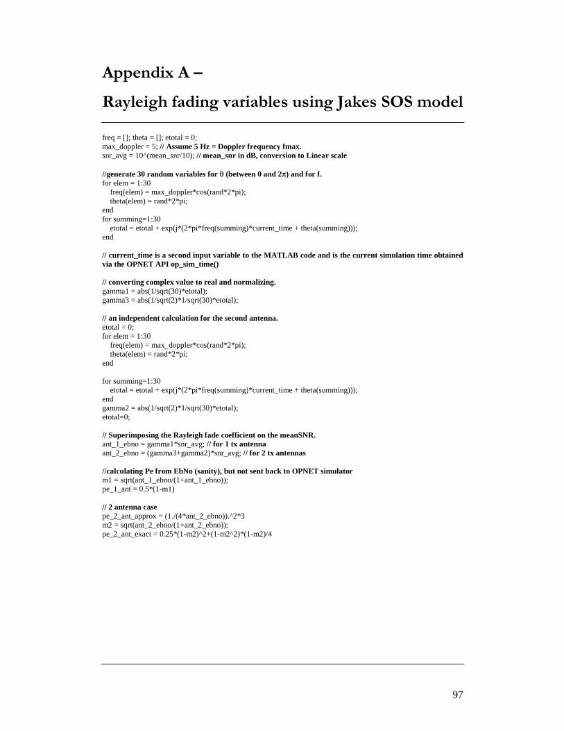
97

Appendix A –

Rayleigh fading variables using Jakes SOS model freq = []; theta = []; etotal = 0; max_doppler = 5; // Assume 5 Hz = Doppler frequency fmax. snr_avg = 10^(mean_snr/10); // mean_snr in dB, conversion to Linear scale //generate 30 random variables for θ (between 0 and 2π) and for f. for elem = 1:30 freq(elem) = max_doppler*cos(rand*2*pi); theta(elem) = rand*2*pi; end for summing=1:30 etotal = etotal + exp(j*(2*pi*freq(summing)*current_time + theta(summing))); end

// current_time is a second input variable to the MATLAB code and is the current simulation time obtained via the OPNET API op_sim_time() // converting complex value to real and normalizing. gamma1 = abs(1/sqrt(30)*etotal); gamma3 = abs(1/sqrt(2)*1/sqrt(30)*etotal); // an independent calculation for the second antenna. etotal = 0; for elem = 1:30 freq(elem) = max_doppler*cos(rand*2*pi); theta(elem) = rand*2*pi; end

for summing=1:30 etotal = etotal + exp(j*(2*pi*freq(summing)*current_time + theta(summing))); end gamma2 = abs(1/sqrt(2)*1/sqrt(30)*etotal); etotal=0; // Superimposing the Rayleigh fade coefficient on the meanSNR. ant_1_ebno = gamma1*snr_avg; // for 1 tx antenna ant_2_ebno = (gamma3+gamma2)*snr_avg; // for 2 tx antennas //calculating Pe from EbNo (sanity), but not sent back to OPNET simulator m1 = sqrt(ant_1_ebno/(1+ant_1_ebno)); pe_1_ant = 0.5*(1-m1) // 2 antenna case pe_2_ant_approx = (1./(4*ant_2_ebno)).^2*3 m2 = sqrt(ant_2_ebno/(1+ant_2_ebno)); pe_2_ant_exact = 0.25*(1-m2)^2+(1-m2^2)*(1-m2)/4

98

Appendix B –

Generation of BER curves R=1/2; i=1; k=1; for x = 0:0.2:15 EbNo=10^(x/10); for d=10:1:17 var_bpsk = 2*d*R*EbNo; %same for QPSK var_qpsk = 2*d*R*EbNo; var_8psk = 0.88*d*R*EbNo; var_16qam = 2*EbNo*R*d*(10^-0.4); var_64qam = 2*EbNo*R*d*(10^-0.8); Pdbpsk(k)=q(sqrt(var_bpsk)); Pdqpsk(k)=q(sqrt(var_qpsk)); Pd8psk(k)=q(sqrt(var_8psk)); Pd16qam(k)=2*q(sqrt(var_16qam)); Pd64qam(k)=2*q(sqrt(var_64qam)); k=k+1; end Pbbpsk(i)=36*Pdbpsk(1) + 211*Pdbpsk(3) +1404*Pdbpsk(5) + 11633*Pdbpsk(7); Pbqpsk(i)=36*Pdqpsk(1) + 211*Pdqpsk(3) +1404*Pdqpsk(5) + 11633*Pdqpsk(7); Pb8psk(i)=36*Pd8psk(1) + 211*Pd8psk(3) +1404*Pd8psk(5) + 11633*Pd8psk(7); Pb16qam(i)=36*Pd16qam(1) + 211*Pd16qam(3) +1404*Pd16qam(5) + 11633*Pd16qam(7); Pb64qam(i)=36*Pd64qam(1) + 211*Pd64qam(3) +1404*Pd64qam(5) + 11633*Pd64qam(7); i=i+1; k=1; end //Generating curves Figure x=0:0.2:15; semilogy(x,Pbbpsk,'-oc'); hold on; semilogy(x,Pbqpsk,'-om'); hold on; semilogy(x,Pb8psk,'-ob'); hold on; semilogy(x,Pb16qam,'-og'); hold on; semilogy(x,Pb64qam,'-ok'); hold on; axis([0 15 10^-6 10^-3])

99

Appendix C –

User scheduling

for (count = 0; count<MAX_USERS; count++) {

current_objid = matlab_interface_objid[count]; //Get Object IDs for each Matlab Interface op_intrpt_force_remote(DRCFB, current_objid); // Interrupt each interface snr_val_recd = (double *)op_ima_obj_svar_get(current_objid,"snrval"); snrvalatbts[count2] = *snr_val_recd; // Get SNR value for user.

} // Select the highest among the different users. for (count2=0; count2<MAX_USERS; count2++) {

if (count2==0) { max = count2; max_val = snrvalatbts[count2]; } else if (snrvalatbts[count2]>=max_val) { max = count2; max_val = snrvalatbts[count2]; }

} // Schedule user…..

100

Appendix D –

THP based multi-user scheduling

for PT=0:0 % in dBW snr=10^(PT/10); % in Watts ram_emus2a_zfthp_txiid end Cthp=load('CthpCooling.txt'); K=10; % nbr. of active uers nt=4; % # of tx antennas ns=min(K,nt); % # of users selected nr=1; % # of rx antennas at each user Tc = 100; % scale of interest in blocks % [20 40 80 100] for 50ms/3 blks, or [40 80 160 200] for 25ms/3 blks fs=60; % blk frequency, must be great than 2*fm(max doppler freq) % 60 for 50ms/3 blks, or 120 for 25ms/3 blks nbr_blks = 18000; % 2000 for 5.6Hz-above doppler, 8000 for 1.5Hz doppler krice=0*ones(K,1); % rice factor (absoluate value) alpha0=2*pi/3*rand(K,1); % initial AOA of specular component fm=5.6*ones(K,1); % doppler freq. tr(:,1)=ones(K,1); % init window-averaged user snr (window length=Tc) for blk=1:nbr_blks % user channel realizations for ii=1:nt H(:,ii)=rice_dent1(fm,alpha0,krice,fs,1,0,K,blk,ii); end % greedy scheduling set_gd=zeros(1,ns); % user subset selection, init user subset selection schrate_gd=zeros(ns,1); tmp_gd=0; for k=1:ns tmp_id=0; schrate=zeros(k,1); for ii=1:K if prod(set_gd(1:k-1)-ii)==0 continue; end Hu=H([set_gd(find(set_gd(1:k-1)>0)) ii],:); kid=sum(set_gd>0); HH=Hu*Hu'; HH=diag(real(diag(HH)))+HH.*(ones(kid+1,kid+1)-diag(ones(1,kid+1))); % set diagonal real G=diag(chol(HH)).^2; schrate=interp1(Cthp(:,1),Cthp(:,2),10*log10(snr/(kid+1)*G)); Rind1=find(10*log10(snr/(kid+1)*G)<-20); schrate(Rind1)=6e-3; Rind2=find(10*log10(snr/(kid+1)*G)>30); schrate(Rind2)=log2(6*snr/(kid+1)*G(Rind2)/(pi*exp(1))); sdr_gd=sum(schrate); if sdr_gd>tmp_gd tmp_gd=sdr_gd; tmp_id=ii; schrate_gd=schrate; end end set_gd(k)=tmp_id; if (set_gd(k)==0) break; end end Rgd(blk)=sum(schrate_gd);

101

% round-robin scheduling set_rr=mod((1:ns)+blk-2,K)+1; % round-robin user set fprintf(rr,'%d\t %d\t %d\t %d\t\n',set_rr); Hu=H(set_rr,:); HH=Hu*Hu'; for ii=1:ns HH(ii,ii)=real(HH(ii,ii)); end R=chol(HH); % channel gain for RR scheduling G=diag(R).^2; % optimal noise cooling schrate_rr=interp1(Cthp(:,1),Cthp(:,2),10*log10(snr/ns*G)); Rind1=find(10*log10(snr/ns*G)<-20); schrate_rr(Rind1)=6e-3; Rind2=find(10*log10(snr/ns*G)>30); schrate_rr(Rind2)=log2(6*snr/ns*G(Rind2)/(pi*exp(1))); fprintf(rrsnr,'%d\t %d\t %d\t %d\t\n',schrate_rr); Rrr(blk)=sum(schrate_rr); % proportional-fair scheduling A=zeros(K,1); set_pf=zeros(1,ns); % init user subset selection schrate_pf=zeros(ns,1); % init schrate_pf tmp_pf=0; for k=1:ns tmp_id=0; schrate=zeros(k,1); for ii=1:K if prod(set_pf(1:k-1)-ii)==0 continue; end Hu=H([set_pf(find(set_pf(1:k-1)>0)) ii],:); kid=sum(set_pf>0); HH=Hu*Hu'; HH=diag(real(diag(HH)))+HH.*(ones(kid+1,kid+1)-diag(ones(1,kid+1))); % set diagonal real G=diag(chol(HH)).^2; % optimal noise cooling schrate=interp1(Cthp(:,1),Cthp(:,2),10*log10(snr/(kid+1)*G)); Rind1=find(10*log10(snr/(kid+1)*G)<-20); schrate(Rind1)=6e-3; Rind2=find(10*log10(snr/(kid+1)*G)>30); schrate(Rind2)=log2(6*snr/(kid+1)*G(Rind2)/(pi*exp(1))); sdr_pf=sum(schrate./tr([set_pf(find(set_pf(1:k-1)>0)) ii],blk)); if sdr_pf>tmp_pf tmp_pf=sdr_pf; tmp_id=ii; schrate_pf=schrate; end end set_pf(k)=tmp_id; if (set_pf(k)==0) break; end end fprintf(pf,'%d\t %d\t %d\t %d\t\n',set_pf); fprintf(pfsnr,'%d\t %d\t %d\t %d\t\n',schrate_pf); Rpf(blk)=sum(schrate_pf); A(set_pf(find(set_pf>0)))=schrate_pf; tr(:,blk+1)=(1-1/Tc)*tr(:,blk)+1/Tc*A; end

102

Vita

Ram Parameswaran was born in Vizag, India. He earned his Bachelors of Engineering (B.E)

in Electronics and Telecommunications from the Vivekanand Institute of Science and

Technology (VESIT) affiliated with the University of Bombay. While in the University of

Bombay, he served as the treasurer and then the President of the IEEE-VESIT student branch.

He joined the Bradley Department of Electrical Engineering of Virginia Tech in the fall of

2001 as a Master’s student, where he worked in the Mobile and Portable Radio Research

group (MPRG) under Dr. Mike Buehrer. During the summer of 2002, he worked as an intern

in the Corporate Research and Development group at Qualcomm Inc on the 1xEVDO project.

In Fall 2002, he was awarded the IEEE graduate student fellowship for first year Masters

students in Electrical Engineering. He has been in the UMTS performance test group at

Qualcomm Inc. since August 2003 and works on optimizing their 3G video telephony and

streaming video solution.

His interests include cross layer wireless design, understanding concepts in new wireless

research, and mobile multimedia technology. He is especially interested in learning about

disruptive methods that could change the face wireless communications. He relishes reading

about business strategy, finance, leadership and capitalist philosophy. When work or research

does not keep him busy, he enjoys playing tennis, cooking and constructive debating with the

unfortunate folks who cross his path.