1 Identifying Codes and Covering Problems
34
1 Identifying Codes and Covering Problems Moshe Laifenfeld and Ari Trachtenberg Abstract The identifying code problem for a given graph involves finding a minimum set of vertices whose neighbor- hoods uniquely overlap at any given graph vertex. Initially introduced in 1998, this problem has demonstrated its fundamental nature through a wide variety of applications, such as fault diagnosis, location detection, and environmental monitoring, in addition to deep connections to information theory, superimposed and covering codes, and tilings. This work establishes efficient reductions between the identifying code problem and the well-known set- covering problem, resulting in a tight hardness of approximation result and novel, provably tight polynomial-time approximations. The main results are also extended to r-robust identifying codes and analogous set (2r + 1)- multicover problems. Finally, empirical support is provided for the effectiveness of the proposed approximations, including good constructions for well-known topologies such as infinite two-dimensional grids. Index Terms Identifying codes, robust identifying codes, hardness of approximation, set cover, test cover, distributed algo- rithms. A version of this paper is scheduled to appear as: • M. Laifenfeld and A. Trachtenberg, “Identifying Codes and Covering Problems”, IEEE Transactions on Information Theory, September 2008. I. I NTRODUCTION An identifying code is a subset of vertices in a graph with the property that the (incoming) neighborhood of any vertex has a unique intersection with the code. For example, a three dimensional cube (as depicted in Figure 1) has a three-vertex identifying code (labeled {1, 2, 3} in the figure). The neighborhood of each vertex in the graph intersects uniquely with this code, and such an intersection is called an identifying set 1 ; given an identifying set, one can thus uniquely identify the vertex in the graph that produced it. In this case, the code provided is also optimal, because one needs at least lg 8 = 3 code vertices to produce 8 distinct identifying sets (corresponding to the 8 vertices of the cube). 2 The goal of the identifying code problem is to find an identifying code of minimum cardinality for any given graph. Identifying codes have been studied extensively since their introduction in 1998 [1], and they have formed a fundamental basis for a wide variety of theoretical work and practical applications. This work was supported in part by the National Science Foundation under grants CCR-0133521, CNS-0435312 and CCF-0729158, and in part by DTRA grant HDTRA1-07-1-0004. The material was presented in part at the 44th Allerton Conference on Communication, Control, and Computing, September 2006. The authors ([email protected] and [email protected], respectively) are with the department of Electrical and Computer Engineering, Boston University, Boston MA 02215. The first author is also with the department of Aeronautics and Astronautics, Massachusetts Institute of Technology, Cambridge MA 02139. 1 Unlike traditional identifying codes, the empty set is considered a valid identifying set here. 2 As is common, we use the notation lg(x) to denote log 2 (x).
Transcript of 1 Identifying Codes and Covering Problems

1
Identifying Codes and Covering ProblemsMoshe Laifenfeld and Ari Trachtenberg
Abstract
The identifying code problemfor a given graph involves finding a minimum set of vertices whose neighbor-hoods uniquely overlap at any given graph vertex. Initiallyintroduced in 1998, this problem has demonstratedits fundamental nature through a wide variety of applications, such as fault diagnosis, location detection, andenvironmental monitoring, in addition to deep connectionsto information theory, superimposed and covering codes,and tilings. This work establishes efficient reductions between the identifying code problem and the well-known set-covering problem, resulting in a tight hardness of approximation result and novel, provably tight polynomial-timeapproximations. The main results are also extended tor-robust identifying codes and analogousset (2r + 1)-multicoverproblems. Finally, empirical support is provided for the effectiveness of the proposed approximations,including good constructions for well-known topologies such as infinite two-dimensional grids.
Index Terms
Identifying codes, robust identifying codes, hardness of approximation, set cover, test cover, distributed algo-rithms.
A version of this paper is scheduled to appear as:• M. Laifenfeld and A. Trachtenberg, “Identifying Codes and Covering Problems”, IEEE Transactions
on Information Theory, September 2008.
I. I NTRODUCTION
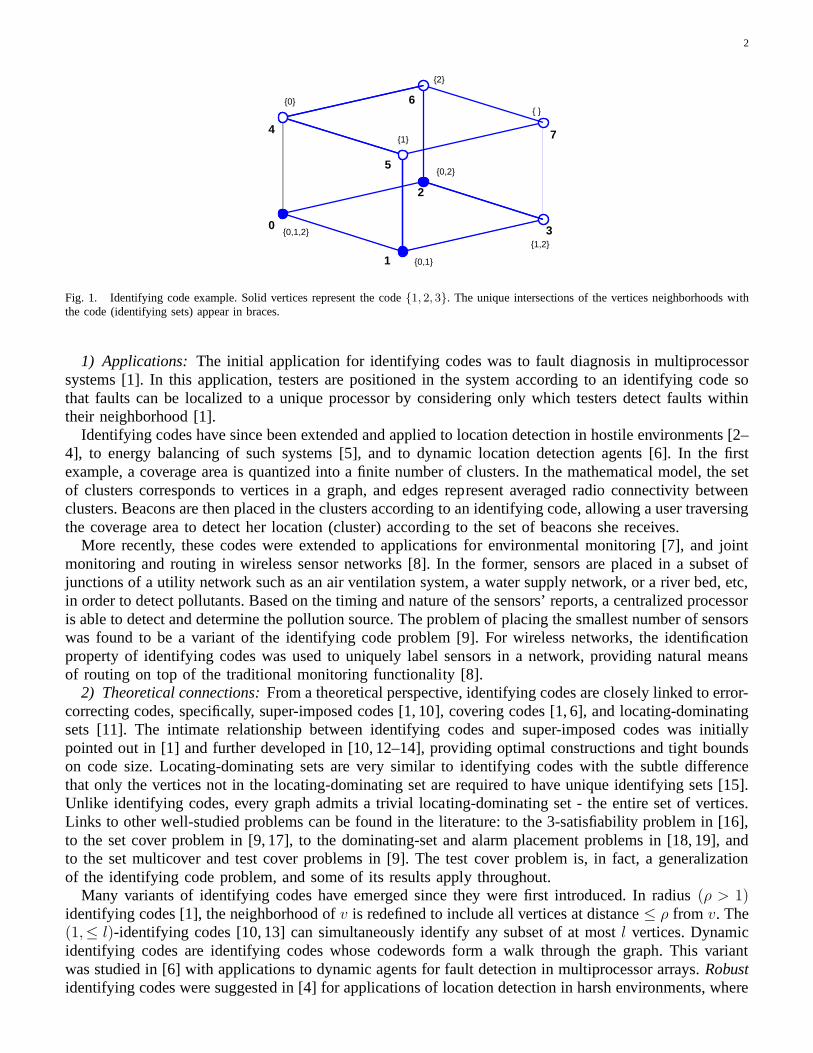
An identifying code is a subset of vertices in a graph with theproperty that the (incoming) neighborhoodof any vertex has a unique intersection with the code. For example, a three dimensional cube (as depictedin Figure 1) has a three-vertex identifying code (labeled{1, 2, 3} in the figure). The neighborhood of eachvertex in the graph intersects uniquely with this code, and such an intersection is called anidentifyingset1; given an identifying set, one can thus uniquely identify the vertex in the graph that produced it. Inthis case, the code provided is also optimal, because one needs at leastlg 8 = 3 code vertices to produce8 distinct identifying sets (corresponding to the8 vertices of the cube).2 The goal of theidentifying codeproblemis to find an identifying code of minimum cardinality for any given graph.
Identifying codes have been studied extensively since their introduction in 1998 [1], and they haveformed a fundamental basis for a wide variety of theoreticalwork and practical applications.
This work was supported in part by the National Science Foundation under grants CCR-0133521, CNS-0435312 and CCF-0729158, and inpart by DTRA grant HDTRA1-07-1-0004. The material was presented in part at the 44th Allerton Conference on Communication, Control,and Computing, September 2006.
The authors ([email protected] and [email protected], respectively) are with the department of Electrical and Computer Engineering, BostonUniversity, Boston MA 02215. The first author is also with thedepartment of Aeronautics and Astronautics, Massachusetts Institute ofTechnology, Cambridge MA 02139.
1Unlike traditional identifying codes, the empty set is considered a valid identifying set here.2As is common, we use the notationlg(x) to denotelog2(x).
2
0
1
2
3
4
5
6
7
{1,2}
{0,1}
{0,1,2}
{0,2}
{ }
{2}
{0}
{1}
Fig. 1. Identifying code example. Solid vertices representthe code{1, 2, 3}. The unique intersections of the vertices neighborhoods withthe code (identifying sets) appear in braces.
1) Applications: The initial application for identifying codes was to fault diagnosis in multiprocessorsystems [1]. In this application, testers are positioned inthe system according to an identifying code sothat faults can be localized to a unique processor by considering only which testers detect faults withintheir neighborhood [1].
Identifying codes have since been extended and applied to location detection in hostile environments [2–4], to energy balancing of such systems [5], and to dynamic location detection agents [6]. In the firstexample, a coverage area is quantized into a finite number of clusters. In the mathematical model, the setof clusters corresponds to vertices in a graph, and edges represent averaged radio connectivity betweenclusters. Beacons are then placed in the clusters accordingto an identifying code, allowing a user traversingthe coverage area to detect her location (cluster) according to the set of beacons she receives.
More recently, these codes were extended to applications for environmental monitoring [7], and jointmonitoring and routing in wireless sensor networks [8]. In the former, sensors are placed in a subset ofjunctions of a utility network such as an air ventilation system, a water supply network, or a river bed, etc,in order to detect pollutants. Based on the timing and natureof the sensors’ reports, a centralized processoris able to detect and determine the pollution source. The problem of placing the smallest number of sensorswas found to be a variant of the identifying code problem [9].For wireless networks, the identificationproperty of identifying codes was used to uniquely label sensors in a network, providing natural meansof routing on top of the traditional monitoring functionality [8].
2) Theoretical connections:From a theoretical perspective, identifying codes are closely linked to error-correcting codes, specifically, super-imposed codes [1, 10], covering codes [1, 6], and locating-dominatingsets [11]. The intimate relationship between identifying codes and super-imposed codes was initiallypointed out in [1] and further developed in [10, 12–14], providing optimal constructions and tight boundson code size. Locating-dominating sets are very similar to identifying codes with the subtle differencethat only the vertices not in the locating-dominating set are required to have unique identifying sets [15].Unlike identifying codes, every graph admits a trivial locating-dominating set - the entire set of vertices.Links to other well-studied problems can be found in the literature: to the 3-satisfiability problem in [16],to the set cover problem in [9, 17], to the dominating-set andalarm placement problems in [18, 19], andto the set multicover and test cover problems in [9]. The testcover problem is, in fact, a generalizationof the identifying code problem, and some of its results apply throughout.
Many variants of identifying codes have emerged since they were first introduced. In radius(ρ > 1)identifying codes [1], the neighborhood ofv is redefined to include all vertices at distance≤ ρ from v. The(1,≤ l)-identifying codes [10, 13] can simultaneously identify any subset of at mostl vertices. Dynamicidentifying codes are identifying codes whose codewords form a walk through the graph. This variantwas studied in [6] with applications to dynamic agents for fault detection in multiprocessor arrays.Robustidentifying codes were suggested in [4] for applications oflocation detection in harsh environments, where

3
vertices and connecting edges are likely to fail. Intuitively, an r-robust identifying code is a code thatmaintains its identification property in the event of a removal or insertion of up tor different verticesfrom all identifying sets. In the example of Figure 1, the setof all vertices forms a 1-robust identifyingcode for the cube. The observation thatr-robust identifying codes are error correcting codes of minimumHamming distance of2r + 1 was made in [4]. Theoretical bounds closely related to covering codes, andsome efficient constructions for periodic geometries were further developed in [6]. Finally, the sourceidentification problem, a variant through which the source of pollutant (traveling according to a givengraph) is to be identified, has been shown to be NP-complete for both the general version [9] and atime-constrained version [7].
3) Approximating the optimal identifying code:In the most general situation, finding a minimum sizeidentifying code for arbitrary undirected and directed graphs was proven to be NP-complete in [16, 20],based on a reduction from the 3-satisfiability problem [21].An exception to this result is the specific caseof directed [22] and undirected trees, for which there exists a polynomial-time algorithm for finding aminimum radius1 identifying code.
Significant efforts in the research of identifying codes andtheir variants have focused on finding efficientconstructions in two dimensional lattices, grids and Hamming spaces (see [12, 23–26], and [6] for a sum-mary of recent results). Until recently, little has been published towards a polynomial time approximationalgorithm for arbitrary graphs. In [2, 4] a polynomial-timegreedy heuristic and its distributed variant weresuggested for obtaining an identifying code in an arbitrarygraph, and simulations showed it to work wellover random graphs. Unfortunately, no guarantees for the quality of the obtained solution were presented,and Moncel later proved in [27] that no such guarantees exist.
Independently and in parallel, several groups have been looking into the question of approximability ofidentifying codes [9, 17, 18], obtaining polynomial-time approximations within anO(log |V |) factor of theoptimal solution. In [18] the authors tied identifying codes to the dominating set problem, thereby showingthat, under common complexity assumptions, approximatingidentifying codes within a sub-logarithmicfactor is intractable. More precisely, it has been shown that identifying codes can be approximated withinO(log |V |) factor, but they can not be approximated in polynomial time within 1 + α log |V | factor forsomeα > 0. In our initial work [9], we have provided an explicit value for α by demonstrating thatidentifying codes are not approximable within aln |V | factor unless NP⊂ DTIMElog log |V |; our resultis based on a reduction from the set cover problem, and we use it to carry over the hardness result ofFeige [28]. In this paper we further show that this bound is tight by adapting an algorithm developed byBerman et al. in [29] that attains this bound within a small additive constant. Using our reduction andwith some additional work, other set cover hardness results(e.g., [30]) may also be applied, obtainingrelated, but distinctly different, results. We also address the approximability of robust identifying codesby establishing a link to the set multi-cover problem.
A. Contributions
The main contribution of this work is to provide good polynomial time approximations to the identifyingcode problem, and to address the fundamental theoretical limits of such approximations. Specifically, weshow that no polynomial-time algorithm can approximate identifying codes onarbitrary graphswithin aln |V | factor under commonly used complexity assumptions. Moreover, we show that a known test coveringapproximation [29] can be adapted to find identifying codes whose size is within a1 + ln |V | factor ofoptimal. The same fundamental questions were researched byothers in parallel and independently [17,18] providing similar, but weaker, results.
Our second contribution in this work is to provide good approximations to the robust identifying codesproblem by tying it to the set multicover problem. Our approximation is guaranteed to produce robustidentifying codes that are within a factor of 2 of the theoretical limit. We also develop two flavors ofdistributed algorithms that may be used for practical implementations in network applications.
4
B. Organization
The rest of the paper is organized as follows: We give formal definitions of the identifying code andthe set cover problems in Section II. In Section III, we show areduction from the set cover problem.In Section IV, we provide anO(log n)-approximation algorithm for the identifying code problem, basedon our reduction, and we show that this approximation ratio is tight. We then generalize this result inSection V, providing a hardness of approximation result forthe identifying code problem, together with anapproximation (based on [29]), which attains this bound up to a small additive constant. In Section VI, wediscuss robust identifying codes and provide an approximation based on their relation to the set multi-coverproblem. Finally in Section VI, we provide distributed implementations of our approximation algorithm,in addition to simulations results on random graphs and grids.
II. FORMAL DEFINITIONS AND RELATED WORK
A. Identifying codes
Given a directed graphG = (V,E), the incoming ballB+(v) consists of vertices that have an edgedirected towardsv ∈ V , together withv; likewise, theoutgoing ballB−(v) consists of vertices that havean edge directed away fromv, together withv. For undirected graphs, we shall simply use the notationB(v) = B+(v) = B−(v).
As such, an identifying code is a set of vertices in a graphG with the property that any incoming ballin G has a unique intersection with the identifying code. More precisely, a non-empty subsetC ⊆ V iscalled acodeand its elements arecodewords. For a given codeC, the identifying setIC(v) of a vertexv is defined to be the codewords directed towardsv, i.e., IC(v) = B+(v) ∩ C (if C is not specified, it isassumed to be the set of all verticesV ). A codeC is thus anidentifying codeif each identifying set ofthe code is unique, or in other words∀u, v ∈ V u = v ←→ IC(u) = IC(v). Note that this definitiondoes not include the standard assumption (which we will makein Section VI) that all identifying sets arenon-empty.
1) Random graphs:Recently, random graphs and random geometric graphs were studied in the contextof identifying codes [14, 31]. In [14] it was shown that for asymptotically large random graphs, any subsetof a certain threshold size (logarithmic in the size of the graph) is almost surely an identifying code. Itwas also shown that the threshold is asymptotically sharp,i.e., the probability of finding an identifyingcode of slightly smaller size asymptotically approaches zero. Unit disk geometric random graphs, in whichvertices are placed on a two-dimensional plane and connected if their distance is less than some unit,were studied in [31]. There it was shown that, unlike large random graphs, most of the large unit-diskgeometric random graphs do not possess identifying codes.
In contrast to very large random graphs, finding a minimum size identifying code for arbitrary undirectedand directed graphs was proven to be NP-complete in [16, 20],based on a reduction from the 3-satisfiabilityproblem.
2) Approximations:An initial attempt to develop a polynomial-time approximation was made in [2, 4].Although the approximation worked well over random graphs it was later proven in [27] to have no generalguarantees for the quality of the obtained solution. More recently, several groups have been independentlylooking into the question of approximability of identifying codes and dominating - locating sets [9, 17,18], providing hardness of approximation results and polynomial time algorithms that approximate theoptimal identifying code within aO(log |V |) factor.
B. Covering problems
1) Set cover:Let U be a base set ofm elements and letS be a family of subsets3 of U. A coverC ⊆ S is a family of subsets whose union isU. Theset cover problemasks to find a coverC of smallestcardinality. The set cover problem is one of the oldest and most studied NP-hard problems [21]. It admits
3The term “family of subsets” is used to refer to a set of subsets
5
the following greedy approximation: at each step, and untilexhaustion, choose the heretofore unselectedset inS that covers the largest number of uncovered elements in the base set.
The performance ratio of the greedy set cover algorithm has also been well-studied. The classic resultsof Lovasz and Johnson [32, 33] showed thatsgreedy/smin = Θ(ln m), wheresmin and sgreedy are theminimum and the greedy covers, andm is the size of the base set. Later Slavik [34] sharpened this ratiofurther, reaching a difference of less than1.1 between the lower and upper bounds on the performanceratio. Recent studies on the hardness of approximation of the set cover problem can be found in [28, 30].Raz and Safra [30] showed that the set cover problem is NP-hard and that it can not be approximatedby a polynomial algorithm within aO(log m) factor from an optimal solution unless P=NP. A tighterresult was obtained by Feige [28] who showed that for anyǫ > 0, no polynomial-time algorithm canapproximate the minimum set cover within(1 − ǫ) ln m factor unless NP has deterministic algorithmsoperating in slightly super-polynomial time,i.e., NP⊂ TIME
[
mO(log log m)]
, suggesting that the greedyapproach is one of the best polynomial approximations to theproblem.
2) Multicover: The minimum setk-multicoverproblem is a natural generalization of the minimum setcover problem, in which one is given a pair(U,S) and seeks the smallest subset ofS that covers everyelement inU at leastk times (we defer more formal definitions to section VI). Oftenthis problem isaddressed as a special case of a more general family of integer optimization problems - thecoveringinteger problem[35, 36].
The set multicover problem admits a similar greedy heuristic to the set cover problem: in each iterationselect the set which covers the maximum number of nonk-multicovered elements. It is well known [36]that the performance guarantee of this heuristic is upper bounded by1 + log α, whereα is the largestset’s size.
3) Test cover:Another closely related problem is thetest cover problem. This problem asks to findthe smallest setT of given testsTi ⊂ U such that any pairx, y ∈ U is differentiated by at least one testTi ∈ T (i.e., |{x, y} ∩ Ti| = 1). The test covering problem appears naturally in identification problems,with roots in an agricultural study more than 20 years ago, regaining interest recently due to applicationsin bioinformatics [37, 38].
Garey and Johnson [39] showed the test cover problem to be NP-hard and later Moret and Shapiro [40]suggested greedy approximations based on a reduction to theset cover problem. More recent work [37,38] studied different branch-and-bound approximations and established a hardness of approximation byextending the reduction in [40], and using a result of Feige [28]. Berman et al. [29] also suggested a novelgreedy approximation and showed its performance ratio to bewithin a small constant from the hardnessresult of [38].
The test cover is clearly a general case of the identifying code problem, with tests corresponding tooutgoing balls, and as such many of its results can be applieddirectly e.g., [29]. Other results, such asthe hardness of approximation, require some work due to the dependencies imposed by graph geographyon nearby identifying sets. As such, the approach we use in Section IV bears some clear similarities tothat of [37].
III. I DENTIFYING CODES AND THE SET COVER PROBLEM
In this section, we establish a reduction between the identifying codes and the set cover problems. Thisreduction will serve as a basis for our subsequent approximation algorithms.
Formally, we connect the following problems:a) SET-COVER:
INSTANCE: SetS of subsets of a base setU .SOLUTION: A set S ′ ⊆ S such that∪s∈S′s = U .MEASURE: The size of the cover:|S ′|.

6
b) ID-CODE:INSTANCE: GraphG = (V, E).SOLUTION: A set C ⊆ V that is an identifying code ofG.MEASURE: The size of the identifying code:|C|.
A. ID-CODE≤P SET-COVER
We first show a reduction from the minimum identifying code problem to the set cover problem. Westate the main theorem first and then we provide several definitions and lemmas that are used in its proof.
Theorem 1 Given a graphG of n vertices, finding an identifying code requires no more computationsthan a set cover solution over a base set ofn(n−1)
2elements together withO(n3) operations (scalar
multiplications, additions, or comparisons) on lengthn binary vectors.
Intuitively, the reduction to a(U,S) set cover problem is established by settingU to contain all pairsof distinct vertices andS = {Sv∈V } to be the set ofSv subsets that contain all pairs such thatv is in theincoming ball of exactly one of them. We start with some notation and formal definitions to bootstrap thereduction.
Definition 1 The difference setD(u, v) is defined to be the symmetric difference between the incomingballs of verticesu, v ∈ V :
D(u, v).= B+(u)⊕ B+(v)
=[
B+(u)−B+(v)]
∪[
B+(v)−B+(u)]
,
where subtraction denotes set difference. We shall also denote byDC(u, v) the intersection of the codeCwith D(u, v), namelyDC(u, v) = D(u, v) ∩ C.
It is easy to see thatDC(u, v) is the symmetric difference between the identifying sets ofverticesu, v ∈ V , namely
DC(u, v) = IC(u)⊕ IC(v).
We shall also useU to denote the set of all pairs of distinct vertices,i.e., U = {(u, z)|u 6= z ∈ V }.Finally, thedistinguishing setof a vertexv ∈ V is the set of vertex pairs(u, z) for whichv is a member
of their difference set:δv = {(u, z) ∈ U | v ∈ D(u, z)}.
Note that the distinguishing set is independent of the codeC.The following Lemma follows trivially from the definition ofan identifying code.
Lemma 1 A codeC is an identifying code iff∅ 6∈ {DC(u, z)|(u, z) ∈ U }.
Alternatively, we can define an identifying code in terms of distinguishing sets.
Lemma 2 C is an identifying code iff the family of the distinguishing sets of its vertices coversU ={(u, z) ∈ V 2 |u 6= z}.
Proof: From Lemma 1 forC to be an identifying code all difference sets should have at least onemember. From the definition of distinguishing sets it then follows that for any(u, v) ∈ U there existssomec ∈ C such that(u, v) ∈ δc. Hence
⋃
c∈Cδc = U . The other direction follows similarly.
Proof of Theorem 1: Consider the following construction of an identifying code.ID(G)→ C.1) Compute the identifying sets{I(u) | u ∈ V }.
7
2) Compute the distinguishing sets∆ = {δu |u ∈ V }.3) ComputeC← Minimum− Set− Cover(U , ∆).4) OutputC ← {u ∈ V | δu ∈ C}, i.e., vertices corresponding to distinguishing sets in the minimum
cover.The resulting code,C, is guaranteed by Lemma 2 to be an identifying code, and the optimality of theset cover in step 3 guarantees that no smaller identifying code can be found. To complete the proof, weobserve that computing the identifying setsI(u) naively requiresΘ(n2) additions of binary vectors, andcomputing∆ requiresn operations for each of then(n−1)
2elements in|U |.
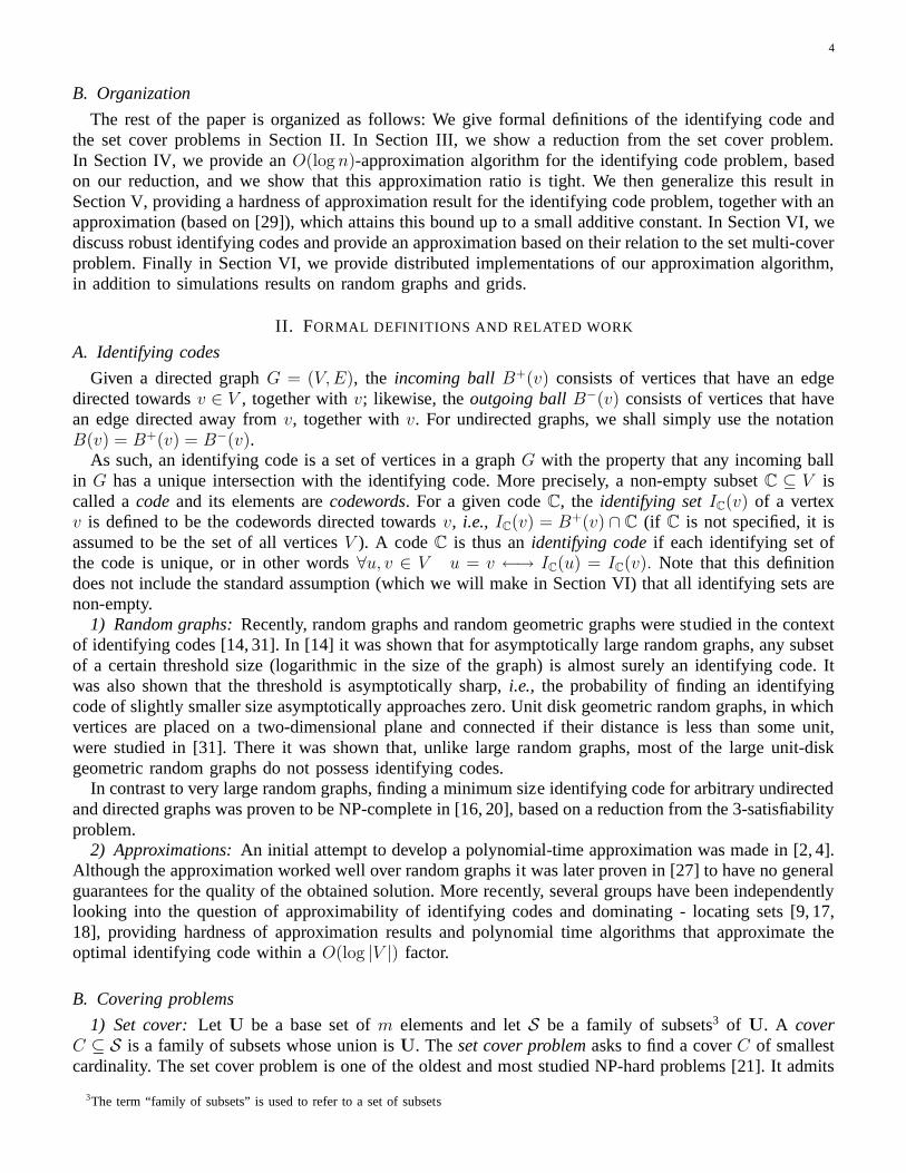
As a simple example of the construction behind Theorem 1, consider the graph in Figure 1. Theidentifying sets and distinguishing sets of the vertices are:
v ∈ V I(v) δv
0 {0,1,2,4}{(0,3),(0,5),(0,6),(0,7),(1,3),(1,5),. . .}1 {0,1,3,5}{(0,2),(0,4),(0,6),(0,7),(1,2),(1,4),. . .}2 {0,2,3,6}{(0,1),(0,4),(0,6),(0,7),(1,0),(1,2),. . .}3 {1,2,3,7}
4 {0,4,5,6}...
5 {1,4,5,7}6 {2,4,6,7}7 {3,5,6,7}
The corresponding set-cover problem would be taken over a base set{(u, z)|0 ≤ u 6= z ≤ 7} andsubset family consisting of all theδv in the table.
B. SET-COVER≤P ID-CODE
We next reduce an identifying code problem to a set cover problem.
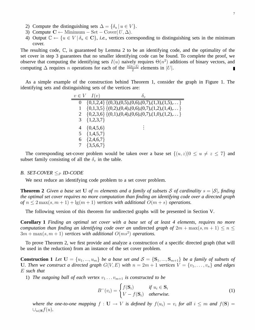
Theorem 2 Given a base setU of m elements and a family of subsetsS of cardinality s = |S|, findingthe optimal set cover requires no more computation than finding an identifying code over a directed graphof n ≤ 2 max(s, m + 1) + lg(m + 1) vertices with additionalO(m + s) operations.
The following version of this theorem for undirected graphswill be presented in Section V.
Corollary 1 Finding an optimal set cover with a base set of at least 4 elements, requires no morecomputation than finding an identifying code over anundirectedgraph of 2m + max(s,m + 1) ≤ n ≤3m + max(s,m + 1) vertices with additionalO(ms2) operations.
To prove Theorem 2, we first provide and analyze a construction of a specific directed graph (that willbe used in the reduction) from an instance of the set cover problem.
Construction 1 Let U = {u1, ..., um} be a base set andS = {S1, ...,Sm+1} be a family of subsets ofU. Then we construct a directed graphG(V, E) with n = 2m + 1 verticesV = {v1, . . . , vn} and edgesE such that
1) The outgoing ball of each vertexv1 . . . vm+1 is constructed to be
B−(vi) =
{
f(Si) if ui ∈ Si
V − f(Si) otherwise.(1)
where the one-to-one mappingf : U → V is defined byf(ui) = vi for all i ≤ m and f(S) =∪u∈Sf(u).

8
U v{= 1 v , 2 v , 3 S } 1 v{= 1 S ,} 2 v{= 1 v, 2 S ,} 3 v{= 2 S ,} 4 v{= 1 v, 3}
v1
v2
v3
v5
v6
v7
v4
v{ 1 v , 2 v , 3 v, 5}
v{ 2 v , 4 v, 6}
v{ 3 v , 7}
v{ 3 v , 4}
v{ 3 v , 4 v, 5}
v{ 3 v , 4 v, 6}
v{ 3 v , 4 v, 7}
Fig. 2. An example of our reduction framework. Incoming balls are noted near their corresponding vertices.
2) The outgoing balls of the remaining verticesvm+2 . . . vn are constructed to be:
B−(vi) = {vi, vi−m−1}.
We next provide several properties of an arbitrary identifying codeC for the graphG(V,E); it might beuseful to refer to Figure 2, which demonstrates our construction on a simple example, when reading theseproperties. Recall that we use the notationD(vi, vj) to denote the difference set of the pair(vi, vj) ∈ V ,and the notationδvi
to denote the distinguishing set of vertexvi. We introduce as additional notation theset←→U = {(vi, vi+m+1) | i ≤ m} and corresponding operator
←→δ = δ ∩
←→U .
Property 1 Any identifying code ofG(V, E) must contain all verticesvm+2 . . . vn.
Property 2 For all k ≥ m + 2, the distinguishing set←→δvk
is empty.
Property 3 C is an identifying code if and only if{vm+2 . . . vn} ⊆ C and {←→δvi| i ≤ m + 1 and vi ∈ C}
is a cover of←→U .
Proof of Properties 1-3: By constructionB+(vm+1) does not contain any vertex of index larger thanm+1, namelyB+(vm+1)∩{vm+2, ..., vn} = ∅. For the rest,i.e., j ≤ m+1, vj is in B+(vm+1) if and onlyif vj ∈ B+(vi) for all i ≥ m + 2. It follows that the difference setsD(vm+1, vi) = {vi} for all i ≥ m + 2.To complete the proof of Property 1 we use Lemma 2 that impliesthat{vi|i ≥ m+2} must be containedin any identifying codeC .
Property 2 is straightforward.To prove the forward direction of Property 3, note that Lemma2 implies that
←−→δv∈C covers
←→U . However,
Property 2 gives that←→δvk
= ∅ for all k > m + 1, and what remains, together with Property 1 completesthis direction of the proof.
For the converse direction, we show that the latter two conditions in the property statement imply thatall difference sets are non-empty, so that Lemma 1 applies toshow thatC is an identifying code. Wefirst considerDC(vi, vj) where (vi, vj) ∈
←→U ; for such pairs in
←→U , our construction provides thatvi is
either in the identifying setIC(vi) or else inIC(vj), so thatDC(vi, vj) 6= ∅ for all (vi, vj) ∈←→U . For pairs
(vi, vj) 6∈←→U and allC , we observe that
D(vi, vj) ∩ {vm+2, ..., vn} 6= ∅, (2)
by considering two possibilities fori (assumed< j without loss of generality): (i)i ≤ m, whereinIC(vi)containsvi+m+1 andIC(vj) cannot; or (ii)j > m + 1, whereinIC(vj) containsvj andIC(vi) cannot.
9
Note that Property 3 produces a one-to-one correspondence between identifying codes and set coversusing distinguishing sets, so that, in fact, a minimum identifying code produces a minimum set cover. Wenext make use of this property to relate identifying codes tothe original subsetsS.
The family of distinguishing sets{←→δvi|i ≤ m + 1} over the support
←→U is equivalent to the original
family of subsetsS over the supportU. We use this to develop the following lemma.
Lemma 3 C is an identifying code ofG(V,E) if and only if {vm+2 . . . vn} ⊆ C and {Si | vi ∈ C, i ≤m + 1} is a set cover of(U,S).
Proof: Based on Property 3, all we need to show is that there is a one-to-one mapping between thefamily of distinguishing sets{
←→δvi|i ≤ m + 1} over the support
←→U and the original family of subsetsS
over the supportU. In the following the indicesi, j are taken to bei ≤ m+1, andj ≤ m. By constructionif uj /∈ Si then verticesvj and vj+m+1 are either both in or both not inB−(vi) . Otherwise ifuj ∈ Si
then only one of them is inB−(vi). It follows that (vj, vj+m+1) ∈ δviif and only if uj ∈ Si, completing
the proof.
Proof of Theorem 2: Given a base setU of sizem and a family of subsetsS of sizes, we triviallyproduce setsU′ and S ′ that fit Construction 1 as follows: (i) ifs < m + 1, thenU
′ is derived fromU
by padding it withx new items, wherex is the smallest integer satisfyingm + x + 1 ≤ s + 2x, andS ′ isderived fromS by addingm+x+1−s distinct subsets of these new items (note thatx < 1+lg m+1); (ii)otherwise,U′ is derived fromU by padding it withs− 1−m new items, and these items are also addedto each set inS to form S ′. Lemma 3 then assures that a minimum identifying code of the generatedgraph corresponds to a minimum set cover of(U, S).
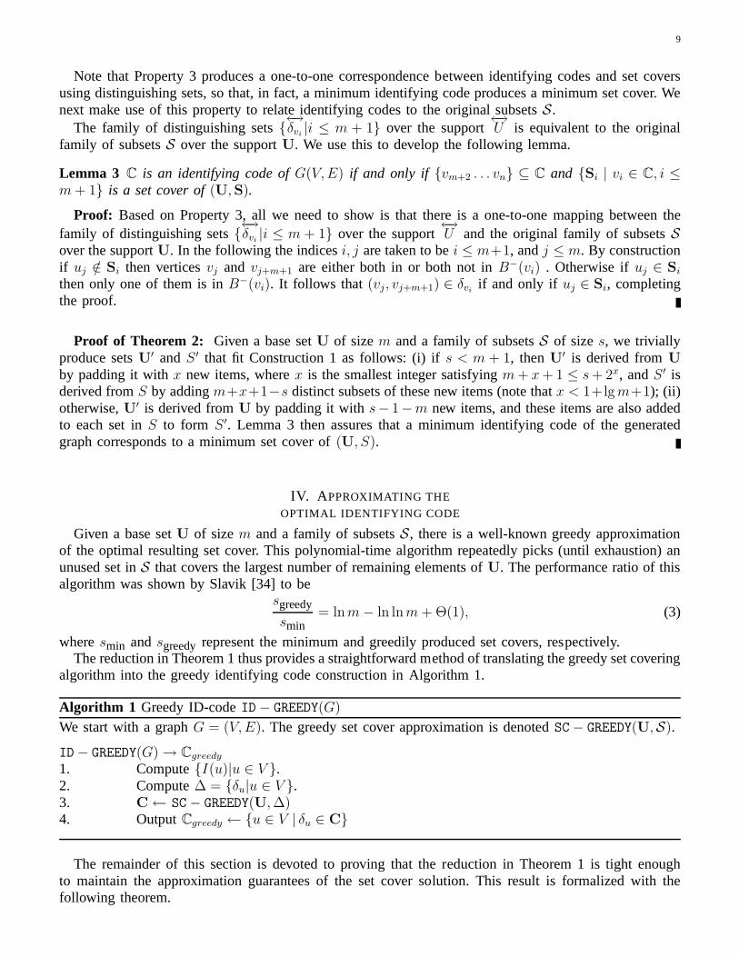
IV. A PPROXIMATING THE
OPTIMAL IDENTIFYING CODE
Given a base setU of sizem and a family of subsetsS, there is a well-known greedy approximationof the optimal resulting set cover. This polynomial-time algorithm repeatedly picks (until exhaustion) anunused set inS that covers the largest number of remaining elements ofU. The performance ratio of thisalgorithm was shown by Slavik [34] to be
sgreedy
smin= lnm− ln lnm + Θ(1), (3)
wheresmin andsgreedy represent the minimum and greedily produced set covers, respectively.The reduction in Theorem 1 thus provides a straightforward method of translating the greedy set covering
algorithm into the greedy identifying code construction inAlgorithm 1.
Algorithm 1 Greedy ID-codeID− GREEDY(G)
We start with a graphG = (V, E). The greedy set cover approximation is denotedSC− GREEDY(U,S).
ID− GREEDY(G)→ Cgreedy
1. Compute{I(u)|u ∈ V }.2. Compute∆ = {δu|u ∈ V }.3. C← SC− GREEDY(U, ∆)4. OutputCgreedy ← {u ∈ V | δu ∈ C}
The remainder of this section is devoted to proving that the reduction in Theorem 1 is tight enoughto maintain the approximation guarantees of the set cover solution. This result is formalized with thefollowing theorem.
10
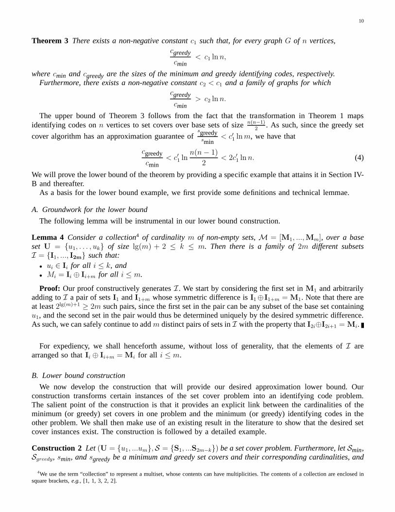
Theorem 3 There exists a non-negative constantc1 such that, for every graphG of n vertices,cgreedy
cmin< c1 ln n,
wherecmin and cgreedyare the sizes of the minimum and greedy identifying codes, respectively.Furthermore, there exists a non-negative constantc2 < c1 and a family of graphs for which
cgreedy
cmin> c2 ln n.
The upper bound of Theorem 3 follows from the fact that the transformation in Theorem 1 mapsidentifying codes onn vertices to set covers over base sets of sizen(n−1)
2. As such, since the greedy set
cover algorithm has an approximation guarantee ofsgreedy
smin< c′1 ln m, we have that
cgreedy
cmin< c′1 ln
n(n− 1)
2< 2c′1 ln n. (4)
We will prove the lower bound of the theorem by providing a specific example that attains it in Section IV-B and thereafter.
As a basis for the lower bound example, we first provide some definitions and technical lemmae.
A. Groundwork for the lower bound
The following lemma will be instrumental in our lower bound construction.
Lemma 4 Consider a collection4 of cardinality m of non-empty sets,M = [M1, ...,Mm], over a baseset U = {u1, . . . , uk} of size lg(m) + 2 ≤ k ≤ m. Then there is a family of2m different subsetsI = {I1, ..., I2m} such that:
• ui ∈ Ii for all i ≤ k, and• Mi = Ii ⊕ Ii+m for all i ≤ m.
Proof: Our proof constructively generatesI. We start by considering the first set inM1 and arbitrarilyadding toI a pair of setsI1 andI1+m whose symmetric difference isI1⊕I1+m = M1. Note that there areat least2lg(m)+1 ≥ 2m such pairs, since the first set in the pair can be any subset of the base set containingu1, and the second set in the pair would thus be determined uniquely by the desired symmetric difference.As such, we can safely continue to addm distinct pairs of sets inI with the property thatI2i⊕I2i+1 = Mi.
For expediency, we shall henceforth assume, without loss ofgenerality, that the elements ofI arearranged so thatIi ⊕ Ii+m = Mi for all i ≤ m.
B. Lower bound construction
We now develop the construction that will provide our desired approximation lower bound. Ourconstruction transforms certain instances of the set coverproblem into an identifying code problem.The salient point of the construction is that it provides an explicit link between the cardinalities of theminimum (or greedy) set covers in one problem and the minimum(or greedy) identifying codes in theother problem. We shall then make use of an existing result inthe literature to show that the desired setcover instances exist. The construction is followed by a detailed example.
Construction 2 Let (U = {u1, ...um},S = {S1, ...S2m−k}) be a set cover problem. Furthermore, letSmin,Sgreedy, smin, andsgreedybe a minimum and greedy set covers and their corresponding cardinalities, and
4We use the term “collection” to represent a multiset, whose contents can have multiplicities. The contents of a collection are enclosed insquare brackets,e.g., [1, 1, 3, 2, 2].
11
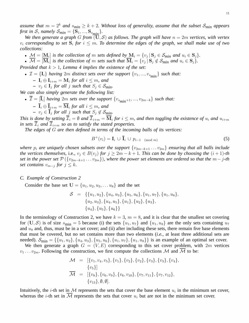
assume thatm = 2k and smin ≥ k + 2. Without loss of generality, assume that the subsetSmin appearsfirst in S, namelySmin = {S1, ...,Ssmin
}.We then generate a graphG from (U,S) as follows. The graph will haven = 2m vertices, with vertex
vi corresponding to setSi for i ≤ m. To determine the edges of the graph, we shall make use of twocollections:
• M = [Mi] is the collection ofm sets defined byMi = {vj |Sj ∈ Smin and ui ∈ Sj}.• M = [Mi] is the collection ofm sets such thatMi = {vj |Sj /∈ Smin and ui ∈ Sj}.
Provided thatk > 1, Lemma 4 implies the existence of the set:• I = {Ii} having2m distinct sets over the support{v1, ..., vsmin
} such that:– Ii ⊕ Ii+m = Mi for all i ≤ m, and– vj ∈ Ij for all j such thatSj ∈ Smin.
We can also simply generate the following list:• I = [Ii] having2m sets over the support{vsmin+1, ..., v2m−k} such that:
– Ii ⊕ Ii+m = Mi for all i ≤ m, and– vj ∈ Ij for all j such thatSj 6∈ Smin.
This is done by settingIi = ∅ andI i+m = Mi for i ≤ m, and then toggling the existence ofui andui+m
in setsIi and Ii+m so as to satisfy the stated properties.The edges ofG are then defined in terms of the incoming balls of its vertices:
B+(vi) = Ii ∪ Ii ∪ pi−1 (mod m) (5)
wherepi are uniquely chosen subsets over the support{v2m−k+1 . . . v2m} ensuring that all balls includethe vertices themselves,i.e., vj ∈ B(vj) for j ≥ 2m− k + 1. This can be done by choosing the(i + 1)-thset in the power setP ({v2m−k+1 . . . v2m}), where the power set elements are ordered so that them− j-thset containsvm−j for j ≤ k.
C. Example of Construction 2
Consider the base setU = {u1, u2, u3, . . . u8} and the set
S = {{u1, u2}, {u4, u3}, {u5, u6}, {u1, u7}, {u1, u8},
{u2, u3}, {u4, u5}, {u1}, {u2}, {u3},
{u4}, {u5}, {u6}}
In the terminology of Construction 2, we havek = 3, m = 8, and it is clear that the smallest set coveringfor (U,S) is of sizesmin = 5 because (i) the sets{u1, u7} and{u1, u8} are the only sets containingu7
andu8 and, thus, must be in a set cover; and (ii) after including these sets, there remain five base elementsthat must be covered, but no set contains more than two elements (i.e., at least three additional sets areneeded).Smin = {{u1, u2}, {u4, u3}, {u5, u6}, {u1, u7}, {u1, u8}} is an example of an optimal set cover.
We then generate a graphG = (V, E) corresponding to this set cover problem, with2m verticesv1 . . . v2m. Following the construction, we first compute the collectionsM andM to be:
M = [{v1, v4, v5}, {v1}, {v2}, {v2}, {v3}, {v3}, {v4},
{v5}]
M = [{v8}, {v6, v9}, {v6, v10}, {v7, v11}, {v7, v12},
{v13}, ∅, ∅].
Intuitively, the i-th set inM represents the sets that cover the base elementui in the minimum set cover,whereas thei-th set inM represents the sets that coverui but are not in the minimum set cover.
12
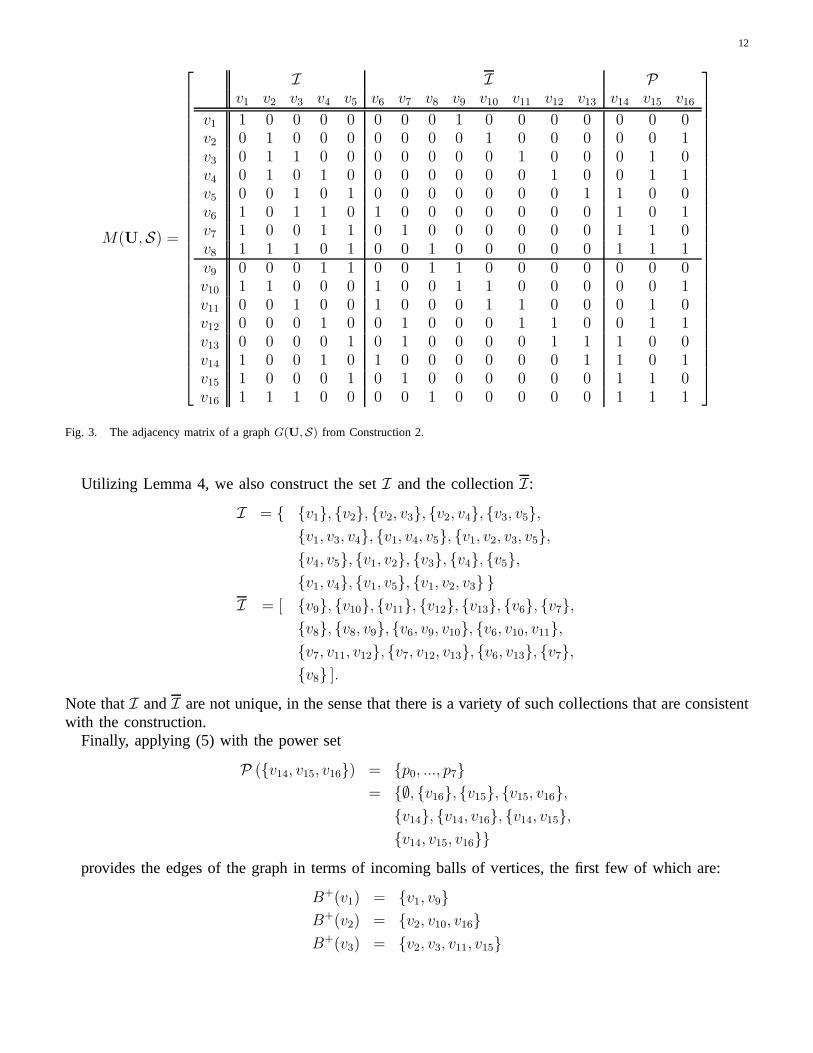
M(U,S) =
I I Pv1 v2 v3 v4 v5 v6 v7 v8 v9 v10 v11 v12 v13 v14 v15 v16
v1 1 0 0 0 0 0 0 0 1 0 0 0 0 0 0 0v2 0 1 0 0 0 0 0 0 0 1 0 0 0 0 0 1v3 0 1 1 0 0 0 0 0 0 0 1 0 0 0 1 0v4 0 1 0 1 0 0 0 0 0 0 0 1 0 0 1 1v5 0 0 1 0 1 0 0 0 0 0 0 0 1 1 0 0v6 1 0 1 1 0 1 0 0 0 0 0 0 0 1 0 1v7 1 0 0 1 1 0 1 0 0 0 0 0 0 1 1 0v8 1 1 1 0 1 0 0 1 0 0 0 0 0 1 1 1v9 0 0 0 1 1 0 0 1 1 0 0 0 0 0 0 0v10 1 1 0 0 0 1 0 0 1 1 0 0 0 0 0 1v11 0 0 1 0 0 1 0 0 0 1 1 0 0 0 1 0v12 0 0 0 1 0 0 1 0 0 0 1 1 0 0 1 1v13 0 0 0 0 1 0 1 0 0 0 0 1 1 1 0 0v14 1 0 0 1 0 1 0 0 0 0 0 0 1 1 0 1v15 1 0 0 0 1 0 1 0 0 0 0 0 0 1 1 0v16 1 1 1 0 0 0 0 1 0 0 0 0 0 1 1 1
Fig. 3. The adjacency matrix of a graphG(U,S) from Construction 2.
Utilizing Lemma 4, we also construct the setI and the collectionI:
I = { {v1}, {v2}, {v2, v3}, {v2, v4}, {v3, v5},
{v1, v3, v4}, {v1, v4, v5}, {v1, v2, v3, v5},
{v4, v5}, {v1, v2}, {v3}, {v4}, {v5},
{v1, v4}, {v1, v5}, {v1, v2, v3} }
I = [ {v9}, {v10}, {v11}, {v12}, {v13}, {v6}, {v7},
{v8}, {v8, v9}, {v6, v9, v10}, {v6, v10, v11},
{v7, v11, v12}, {v7, v12, v13}, {v6, v13}, {v7},
{v8} ].
Note thatI andI are not unique, in the sense that there is a variety of such collections that are consistentwith the construction.
Finally, applying (5) with the power set
P ({v14, v15, v16}) = {p0, ..., p7}
= {∅, {v16}, {v15}, {v15, v16},
{v14}, {v14, v16}, {v14, v15},
{v14, v15, v16}}
provides the edges of the graph in terms of incoming balls of vertices, the first few of which are:
B+(v1) = {v1, v9}
B+(v2) = {v2, v10, v16}
B+(v3) = {v2, v3, v11, v15}

13
It is easier to conceptualize the graph in terms of its adjacency matrix, as depicted in Figure 3. Inthis matrix, each row represents the incoming ball of a vertex. We shall prove with Properties 1- 3 thatcmin = smin andcgreedy= sgreedy+k for this graph, wherecmin andcgreedyare the minimum and greedyidentifying code cardinalities forG(U,S).
D. Lower bound
We next provide some properties of Construction 2 that will be crucial in completing the proof of thelower approximation bound of Theorem 3. Here
←→U = {(vi, vm+i)|i ≤ m}, and recall that
←→δ = δ ∩
←→U .
Property 4 Given a set cover problem(U,S) with |U| = 2k = m, |S| = 2m − k, and smin ≥ k + 2,Construction 2 produces a graphG with the following properties:
1) The verticesVmin = {v1, ..., vsmin} associated withSmin form an identifying code ofG = (V, E).
More precisely,Vmin contains exactly verticesvi, wherei is such thatSi ∈ Smin.2) The distinguishing sets ofV = {v2m−k+1, ..., v2m} ⊆ V cover all pairs of distinct vertices except←→U . More precisely,
⋃
i∈{2m−k+1...2m} δvi=
{(vu, vz) | z 6= u + m and 1 ≤ u < z ≤ 2m}.
3) The modified set cover problem(←→U , {←→δv1
. . .←−−→δv2m−k
}) is equivalent to the original problem(U,S).
As such, the functionf :←→U −→ U wheref ((vi, vi+m)) = ui has the property that
f(←→δvi
) = Si,
with the usual understanding thatf(S) = ∪s∈Sf(s). Note that this also provides an equivalencebetween covers in the modified problem and covers in the original problem.
It may be beneficial to refer to Figure 3 while reading the proof.Proof: The first property follows from the fact that, by design, the sets inI are all different, meaning
that the symmetric difference ofB+(vi) ∩ Vmin andB+(vj) ∩ Vmin is non-empty for all distinct verticesvi andvj . Lemma 1 thus implies thatVmin is an identifying code.
To prove the second property, note that, by construction,B+(vi) ∩ V is unique for every1 ≤ i ≤ m,and similarly for everym + 1 ≤ i ≤ 2m. In fact, only forj = i + m is B+(vi)∩ V = B+(vj)∩ V , henceproving the property.
To prove the third property, we note that, by definition,(vj , vj+m) ∈←→δvi
means thatvi ∈ D(vj, vj+m).By construction the supports ofI andI are disjoint, and their union is{v1, . . . , v2m−k}. Furthermore, bythe construction ofI (andI), (vj, vj+m) ∈
←→δvi
if and only if vi ∈Mj (andMj) wherej ≤ m andvi istaken over the support ofI (I). Therefore by the definition ofM andM it follows that (vj , vj+m) ∈
←→δvi
if and only if uj ∈ Si, completing the proof. Note that this property can be extended to the set of alldistinguishing sets,i.e., {
←→δv1
. . .←−−→δv2m−k
}, if we allow paddingS of the original set cover problem withkempty subsets.
For the next property we need some additional definitions. A code C is said to be a partial code ifC ⊂ C is not an identifying code. Any partial codeC partitions the set of vertices into indistinguishablesubsets,{INDISTi(C)}, where allv ∈ INDISTi(C) have an identical identifying set.
We also need to make aconsistency assumptionin the implementation ofSC− GREEDY, the greedy setcovering algorithm. Specifically, recall thatID− GREEDY calls SC− GREEDY with a base set{(vi, vj)|i 6=j} and a family of subsets{δu}. Our assumption, without loss of generality, will thus be that whenSC− GREEDY must choose between subsetsδu andδv, both covering an equal number of uncovered base el-ements, it will break ties in favor of the first vertex to appear in the precedence list[v2m−k+1, . . . , v2m, v1, . . . , v2m−k].
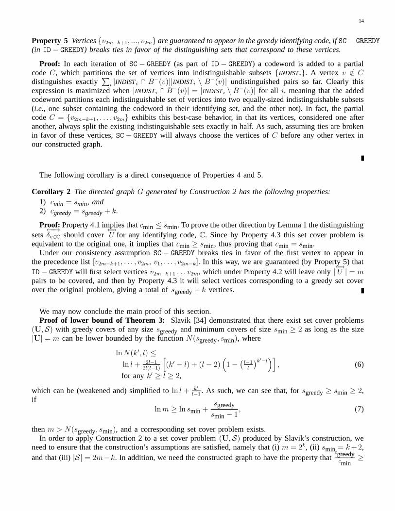
14
Property 5 Vertices{v2m−k+1, ..., v2m} are guaranteed to appear in the greedy identifying code, ifSC− GREEDY
(in ID− GREEDY) breaks ties in favor of the distinguishing sets that correspond to these vertices.
Proof: In each iteration ofSC− GREEDY (as part ofID− GREEDY) a codeword is added to a partialcode C, which partitions the set of vertices into indistinguishable subsets{INDISTi}. A vertex v /∈ Cdistinguishes exactly
∑
i |INDISTi ∩ B−(v)||INDISTi \ B−(v)| undistinguished pairs so far. Clearly thisexpression is maximized when|INDISTi ∩ B−(v)| = |INDISTi \ B−(v)| for all i, meaning that the addedcodeword partitions each indistinguishable set of vertices into two equally-sized indistinguishable subsets(i.e., one subset containing the codeword in their identifying set, and the other not). In fact, the partialcodeC = {v2m−k+1, . . . , v2m} exhibits this best-case behavior, in that its vertices, considered one afteranother, always split the existing indistinguishable setsexactly in half. As such, assuming ties are brokenin favor of these vertices,SC− GREEDY will always choose the vertices ofC before any other vertex inour constructed graph.
The following corollary is a direct consequence of Properties 4 and 5.
Corollary 2 The directed graphG generated by Construction 2 has the following properties:1) cmin = smin, and2) cgreedy= sgreedy+ k.
Proof: Property 4.1 implies thatcmin ≤ smin. To prove the other direction by Lemma 1 the distinguishingsets←−→δv∈C should cover
←→U for any identifying code,C. Since by Property 4.3 this set cover problem is
equivalent to the original one, it implies thatcmin ≥ smin, thus proving thatcmin = smin.Under our consistency assumptionSC− GREEDY breaks ties in favor of the first vertex to appear in
the precedence list[v2m−k+1, . . . , v2m, v1, . . . , v2m−k]. In this way, we are guaranteed (by Property 5) thatID− GREEDY will first select verticesv2m−k+1 . . . v2m, which under Property 4.2 will leave only|
←→U | = m
pairs to be covered, and then by Property 4.3 it will select vertices corresponding to a greedy set coverover the original problem, giving a total ofsgreedy+ k vertices.
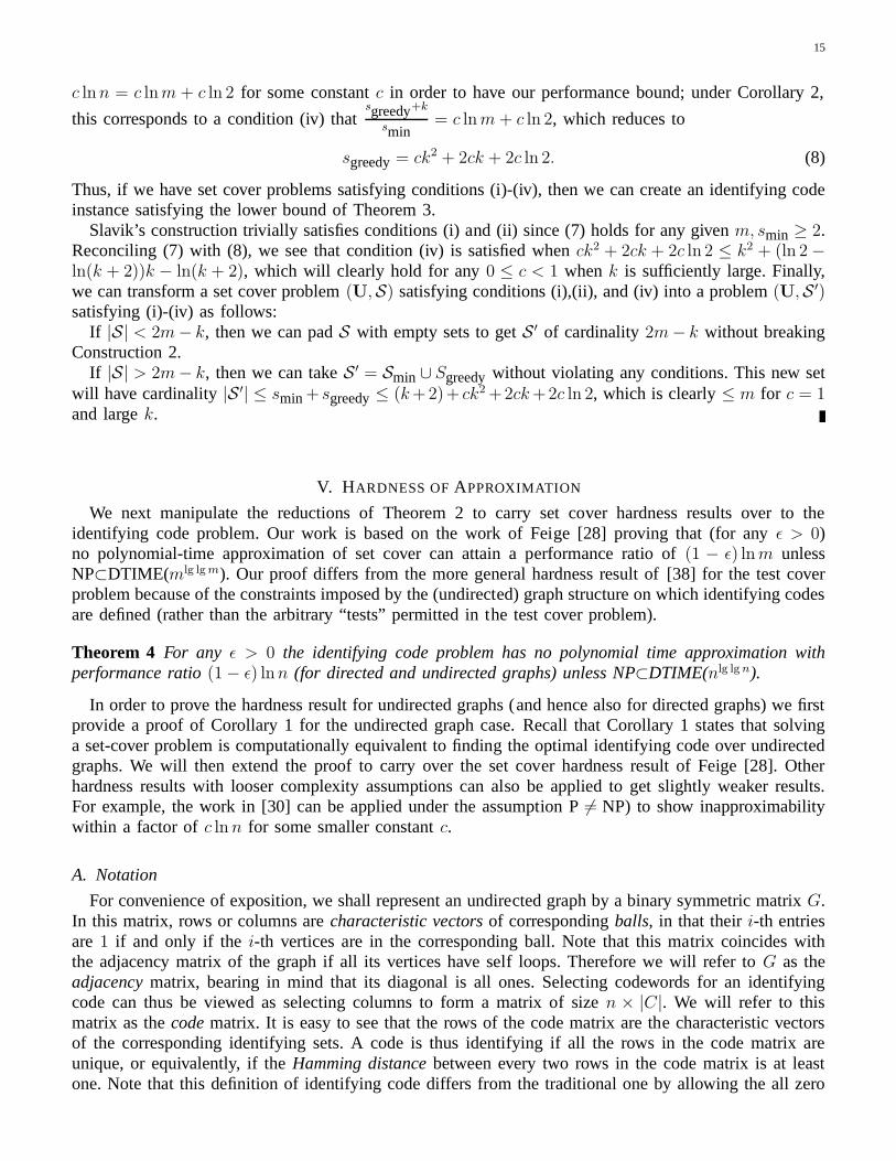
We may now conclude the main proof of this section.Proof of lower bound of Theorem 3: Slavik [34] demonstrated that there exist set cover problems
(U,S) with greedy covers of any sizesgreedyand minimum covers of sizesmin ≥ 2 as long as the size|U| = m can be lower bounded by the functionN(sgreedy, smin), where
ln N(k′, l) ≤
ln l + 2l−12l(l−1)
[
(k′ − l) + (l − 2)(
1−(
l−1l
)k′−l)]
,
for any k′ ≥ l ≥ 2,
(6)
which can be (weakened and) simplified toln l + k′
l−1. As such, we can see that, forsgreedy≥ smin ≥ 2,
ifln m ≥ ln smin +
sgreedy
smin− 1, (7)
thenm > N(sgreedy, smin), and a corresponding set cover problem exists.In order to apply Construction 2 to a set cover problem(U,S) produced by Slavik’s construction, we
need to ensure that the construction’s assumptions are satisfied, namely that (i)m = 2k, (ii) smin = k +2,and that (iii)|S| = 2m−k. In addition, we need the constructed graph to have the property that
cgreedycmin
≥
15
c lnn = c lnm + c ln 2 for some constantc in order to have our performance bound; under Corollary 2,
this corresponds to a condition (iv) thatsgreedy+k
smin= c ln m + c ln 2, which reduces to
sgreedy= ck2 + 2ck + 2c ln 2. (8)
Thus, if we have set cover problems satisfying conditions (i)-(iv), then we can create an identifying codeinstance satisfying the lower bound of Theorem 3.
Slavik’s construction trivially satisfies conditions (i) and (ii) since (7) holds for any givenm, smin ≥ 2.Reconciling (7) with (8), we see that condition (iv) is satisfied whenck2 + 2ck + 2c ln 2 ≤ k2 + (ln 2−ln(k + 2))k − ln(k + 2), which will clearly hold for any0 ≤ c < 1 whenk is sufficiently large. Finally,we can transform a set cover problem(U,S) satisfying conditions (i),(ii), and (iv) into a problem(U,S ′)satisfying (i)-(iv) as follows:
If |S| < 2m− k, then we can padS with empty sets to getS ′ of cardinality2m− k without breakingConstruction 2.
If |S| > 2m− k, then we can takeS ′ = Smin∪ Sgreedywithout violating any conditions. This new setwill have cardinality|S ′| ≤ smin + sgreedy≤ (k +2)+ ck2 +2ck +2c ln 2, which is clearly≤ m for c = 1and largek.
V. HARDNESS OFAPPROXIMATION
We next manipulate the reductions of Theorem 2 to carry set cover hardness results over to theidentifying code problem. Our work is based on the work of Feige [28] proving that (for anyǫ > 0)no polynomial-time approximation of set cover can attain a performance ratio of(1 − ǫ) ln m unlessNP⊂DTIME(mlg lg m). Our proof differs from the more general hardness result of[38] for the test coverproblem because of the constraints imposed by the (undirected) graph structure on which identifying codesare defined (rather than the arbitrary “tests” permitted in the test cover problem).
Theorem 4 For any ǫ > 0 the identifying code problem has no polynomial time approximation withperformance ratio(1− ǫ) lnn (for directed and undirected graphs) unless NP⊂DTIME(nlg lg n).
In order to prove the hardness result for undirected graphs (and hence also for directed graphs) we firstprovide a proof of Corollary 1 for the undirected graph case.Recall that Corollary 1 states that solvinga set-cover problem is computationally equivalent to finding the optimal identifying code over undirectedgraphs. We will then extend the proof to carry over the set cover hardness result of Feige [28]. Otherhardness results with looser complexity assumptions can also be applied to get slightly weaker results.For example, the work in [30] can be applied under the assumption P 6= NP) to show inapproximabilitywithin a factor ofc ln n for some smaller constantc.
A. Notation
For convenience of exposition, we shall represent an undirected graph by a binary symmetric matrixG.In this matrix, rows or columns arecharacteristic vectorsof correspondingballs, in that theiri-th entriesare 1 if and only if the i-th vertices are in the corresponding ball. Note that this matrix coincides withthe adjacency matrix of the graph if all its vertices have self loops. Therefore we will refer toG as theadjacencymatrix, bearing in mind that its diagonal is all ones. Selecting codewords for an identifyingcode can thus be viewed as selecting columns to form a matrix of size n × |C|. We will refer to thismatrix as thecodematrix. It is easy to see that the rows of the code matrix are the characteristic vectorsof the corresponding identifying sets. A code is thus identifying if all the rows in the code matrix areunique, or equivalently, if theHamming distancebetween every two rows in the code matrix is at leastone. Note that this definition of identifying code differs from the traditional one by allowing the all zero
16
G =
100010 Bs
001000111101 Bm
011
,
C7
Bs =
[
0 1100 1010 111
]
Bm =
[
1 0110 1001 0101 001
]
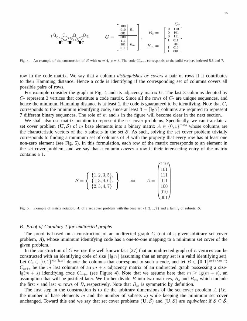
Fig. 4. An example of the construction ofB with m = 4, s = 3. The codeCm+s corresponds to the solid vertices indexed 5,6 and 7.
row in the code matrix. We say that a columndistinguishes or coversa pair of rows if it contributesto their Hamming distance. Hence a code is identifying if thecorresponding set of columns covers allpossible pairs of rows.
For example consider the graph in Fig. 4 and its adjacency matrix G. The last 3 columns denoted byC7 represent 3 vertices that constitute a code matrix. Since all the rows ofC7 are unique sequences, andhence the minimum Hamming distance is at least 1, the code is guaranteed to be identifying. Note thatC7
corresponds to the minimum identifying code, since at least3 = ⌈lg 7⌉ columns are required to represent7 different binary sequences. The role ofm ands in the figure will become clear in the next section.
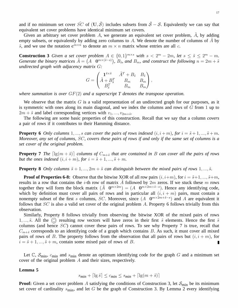
We shall also use matrix notation to represent the set cover problems. Specifically, we can translate aset cover problem(U,S) of m base elements into a binary matrixA ∈ {0, 1}m×s whose columns arethe characteristic vectors of thes subsets in the setS. As such, solving the set cover problem triviallycorresponds to finding a minimum set of columns ofA with the property that every row has at least onenon-zero element (see Fig. 5). In this formulation, each rowof the matrix corresponds to an element inthe set cover problem, and we say that a columncoversa row if their intersecting entry of the matrixcontains a1.
S =
{1, 2, 3, 5},{1, 3, 4, 6},{2, 3, 4, 7}
⇔ A =
110101111011100010001
Fig. 5. Example of matrix notation,A, of a set cover problem with the base set{1, 2, .., 7} and a family of subsets,S.
B. Proof of Corollary 1 for undirected graphs
The proof is based on a construction of an undirected graphG (out of a given arbitrary set coverproblem,A), whose minimum identifying code has a one-to-one mapping to a minimum set cover of thegiven problem.
In the construction ofG we use the well known fact [27] that an undirected graph ofn vertices can beconstructed with an identifying code of size⌈lg n⌉ (assuming that an empty set is a valid identifying set).Let Cn ∈ {0, 1}
n×⌈lg n⌉ denote the columns that correspond to such a code, and letB ∈ {0, 1}m+s×m ⊇Cm+s be them last columns of anm + s adjacency matrix of an undirected graph possessing a size-lg(m + s) identifying codeCm+s (see Figure 4). Note that we assume here thatm ≥ lg(m + s), anassumption that will be justified later. We further divideB into two matrices,Bs andBm, which includethe firsts and lastm rows of B, respectively. Note thatBm is symmetric by definition.
The first step in the construction is to tie the arbitrary dimensions of the set cover problemA (i.e.,the number of base elementsm and the number of subsetss) while keeping the minimum set coverunchanged. Toward this end we say that set cover problems(U, S) and (U,S) are equivalentif S ⊆ S,
17
and if no minimum set coverSC of (U, S) includes subsets fromS − S. Equivalently we can say thatequivalent set cover problems have identical minimum set covers.
Given an arbitrary set cover problemA, we generate an equivalent set cover problem,A, by addingempty subsets, or equivalently by adding zero columns toA. We denote the number of columns ofA bys, and we use the notationcm×n to denote anm× n matrix whose entries are allc.
Construction 3 Given a set cover problemA ∈ {0, 1}m×s with s < 2m − 2m, let s ≤ s ≤ 2m − m.Generate the binary matricesA =
(
A 0m×(s−s)
)
, Bs, andBm, and construct the followingn = 2m + sundirected graph with adjacency matrixG:
G =
1s×s AT + Bs Bs
A + BTs Bm Bm
BTs Bm Bm
,
where summation is overGF (2) and a superscript T denotes the transpose operation.
We observe that the matrixG is a valid representation of an undirected graph for our purposes, as itis symmetric with ones along its main diagonal, and we index the columns and rows ofG from 1 up to2m + s and label corresponding vertices withv1, ..., v2m+s.
The following are some basic properties of this construction. Recall that we say that a columncoversa pair of rows if it contributes to their Hamming distance.
Property 6 Only columns1, ..., s can cover the pairs of rows indexed(i, i + m), for i = s + 1, ..., s + m.Moreover, any set of columns,SC, covers these pairs of rows if and only if the same set of columns is aset cover of the original problem.
Property 7 The ⌈lg(m + s)⌉ columns ofCm+s that are contained inB can cover all the pairs of rowsbut the ones indexed(i, i + m), for i = s + 1, ..., s + m.
Property 8 Only columnss + 1, ..., 2m + s can distinguish between the mixed pairs of rows1, ..., s.
Proof of Properties 6-8: Observe that the bitwise XOR of all row pairs(i, i+m), for i = s+1, ..., s+m,results in a row that contains thei-th row of matrix A followed by 2m zeros. If we stuck thesem rowstogether they will form the block matrix(A 0
m×2m) = (A 0m×2m+s−s). Hence any identifying code,
which by definition must cover all pairs of rows and in particular all (i, i + m) pairs, must contain anonempty subset of the firsts columns,SC. Moreover, since(A 0
m×2m+s−s) and A are equivalent itfollows thatSC is also a valid set cover of the original problemA. Property 6 follows trivially from thisobservation.
Similarly, Property 8 follows trivially from observing thebitwise XOR of the mixed pairs of rows1, ..., s. All the
(
s
2
)
resulting row vectors will have zeros in their firsts elements. Hence the firstscolumns (and henceSC) cannot cover these pairs of rows. To see why Property 7 is true, recall thatCm+s corresponds to an identifying code of a graph which containsB. As such, it must cover all mixedpairs of rows ofB. The property follows from the observation that all pairs ofrows but (i, i + m), fori = s + 1, ..., s + m, contain some mixed pair of rows ofB.
Let C, Smin, cmin and smin denote an optimum identifying code for the graphG and a minimum setcover of the original problemA and their sizes, respectively.
Lemma 5smin + ⌈lg s⌉ ≤ cmin≤ smin + ⌈lg(m + s)⌉
Proof: Given a set cover problemA satisfying the conditions of Construction 3, letSmin be its minimumset cover of cardinalitysmin, and letG be the graph of Construction 3. By Lemma 2 every identifying
18
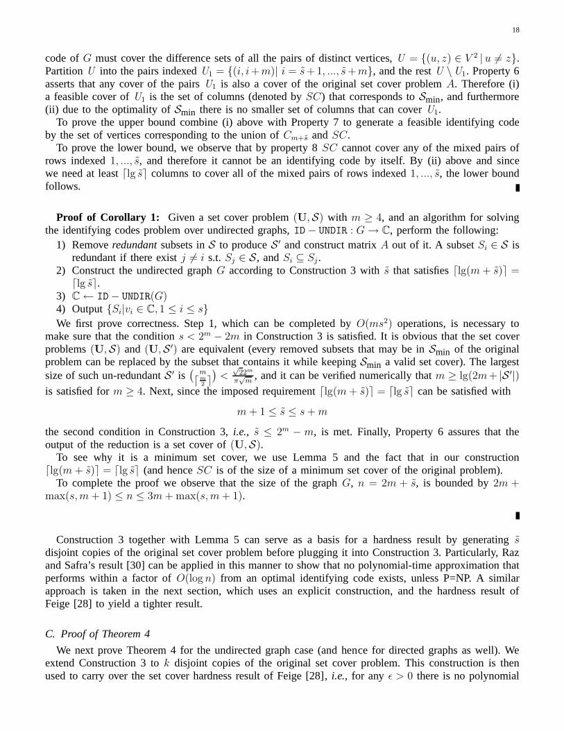
code ofG must cover the difference sets of all the pairs of distinct vertices,U = {(u, z) ∈ V 2 | u 6= z}.PartitionU into the pairs indexedU1 = {(i, i +m)| i = s+1, ..., s +m}, and the restU \U1. Property 6asserts that any cover of the pairsU1 is also a cover of the original set cover problemA. Therefore (i)a feasible cover ofU1 is the set of columns (denoted bySC) that corresponds toSmin, and furthermore(ii) due to the optimality ofSmin there is no smaller set of columns that can coverU1.
To prove the upper bound combine (i) above with Property 7 to generate a feasible identifying codeby the set of vertices corresponding to the union ofCm+s andSC.
To prove the lower bound, we observe that by property 8SC cannot cover any of the mixed pairs ofrows indexed1, ..., s, and therefore it cannot be an identifying code by itself. By(ii) above and sincewe need at least⌈lg s⌉ columns to cover all of the mixed pairs of rows indexed1, ..., s, the lower boundfollows.
Proof of Corollary 1: Given a set cover problem(U,S) with m ≥ 4, and an algorithm for solvingthe identifying codes problem over undirected graphs,ID− UNDIR : G→ C, perform the following:
1) Removeredundantsubsets inS to produceS ′ and construct matrixA out of it. A subsetSi ∈ S isredundant if there existj 6= i s.t. Sj ∈ S, andSi ⊆ Sj .
2) Construct the undirected graphG according to Construction 3 withs that satisfies⌈lg(m + s)⌉ =⌈lg s⌉.
3) C← ID− UNDIR(G)4) Output{Si|vi ∈ C, 1 ≤ i ≤ s}
We first prove correctness. Step 1, which can be completed byO(ms2) operations, is necessary tomake sure that the conditions < 2m − 2m in Construction 3 is satisfied. It is obvious that the set coverproblems(U,S) and (U,S ′) are equivalent (every removed subsets that may be inSmin of the originalproblem can be replaced by the subset that contains it while keepingSmin a valid set cover). The largestsize of such un-redundantS ′ is
(
m
⌈m
2 ⌉)
<√
22m
π√
m, and it can be verified numerically thatm ≥ lg(2m+ |S ′|)
is satisfied form ≥ 4. Next, since the imposed requirement⌈lg(m + s)⌉ = ⌈lg s⌉ can be satisfied with
m + 1 ≤ s ≤ s + m
the second condition in Construction 3,i.e., s ≤ 2m − m, is met. Finally, Property 6 assures that theoutput of the reduction is a set cover of(U,S).
To see why it is a minimum set cover, we use Lemma 5 and the fact that in our construction⌈lg(m + s)⌉ = ⌈lg s⌉ (and henceSC is of the size of a minimum set cover of the original problem).
To complete the proof we observe that the size of the graphG, n = 2m + s, is bounded by2m +max(s, m + 1) ≤ n ≤ 3m + max(s, m + 1).
Construction 3 together with Lemma 5 can serve as a basis for ahardness result by generatingsdisjoint copies of the original set cover problem before plugging it into Construction 3. Particularly, Razand Safra’s result [30] can be applied in this manner to show that no polynomial-time approximation thatperforms within a factor ofO(log n) from an optimal identifying code exists, unless P=NP. A similarapproach is taken in the next section, which uses an explicitconstruction, and the hardness result ofFeige [28] to yield a tighter result.
C. Proof of Theorem 4
We next prove Theorem 4 for the undirected graph case (and hence for directed graphs as well). Weextend Construction 3 tok disjoint copies of the original set cover problem. This construction is thenused to carry over the set cover hardness result of Feige [28], i.e., for any ǫ > 0 there is no polynomial
19
Gk =
I I + AT · · · I + AT AT + Bs BT
s· · · BT
sBs
I + A I. . .
... Bs AT + Bs
. . .... Bs
.... . .
. . . I + AT...
. . .. . . BT
s
...I + A · · · I + A I BT
s· · · BT
sAT + Bs Bs
A + BT
sBT
s· · · BT
sBm Bm · · · Bm Bm
Bs A + BT
s
. . .... Bm Bm Bm Bm
.... . .
. . . BT
s
.... . .
......
Bs · · · Bs A + BT
2 Bm Bm · · · Bm Bm
BT
sBT
s· · · BT
sBm Bm · · · Bm Bm
red1
red2
...redk
blue1
blue2
...bluek
white
Fig. 6. The adjacency matrix of the graphGk in Construction 4.
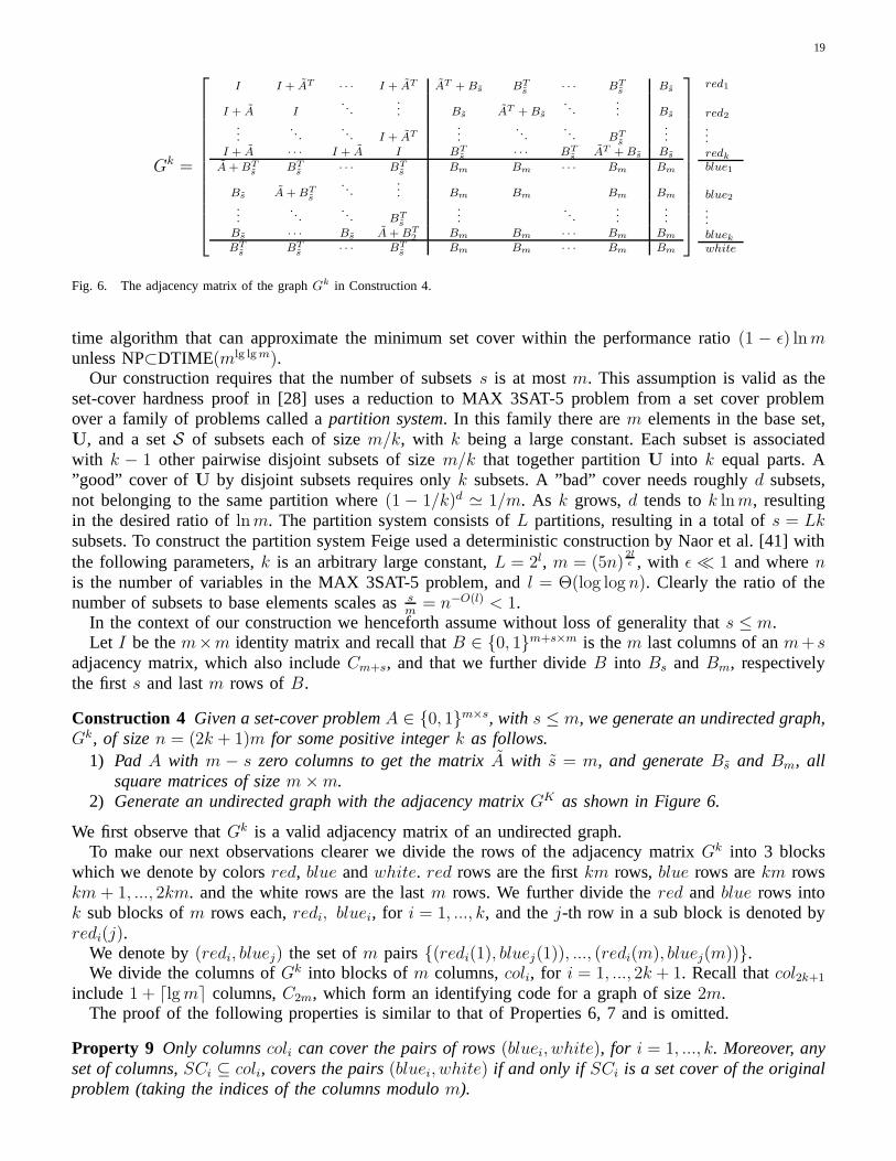
time algorithm that can approximate the minimum set cover within the performance ratio(1 − ǫ) ln munless NP⊂DTIME(mlg lg m).
Our construction requires that the number of subsetss is at mostm. This assumption is valid as theset-cover hardness proof in [28] uses a reduction to MAX 3SAT-5 problem from a set cover problemover a family of problems called apartition system. In this family there arem elements in the base set,U, and a setS of subsets each of sizem/k, with k being a large constant. Each subset is associatedwith k − 1 other pairwise disjoint subsets of sizem/k that together partitionU into k equal parts. A”good” cover ofU by disjoint subsets requires onlyk subsets. A ”bad” cover needs roughlyd subsets,not belonging to the same partition where(1 − 1/k)d ≃ 1/m. As k grows,d tends tok lnm, resultingin the desired ratio ofln m. The partition system consists ofL partitions, resulting in a total ofs = Lksubsets. To construct the partition system Feige used a deterministic construction by Naor et al. [41] withthe following parameters,k is an arbitrary large constant,L = 2l, m = (5n)
2l
ǫ , with ǫ≪ 1 and wherenis the number of variables in the MAX 3SAT-5 problem, andl = Θ(log log n). Clearly the ratio of thenumber of subsets to base elements scales ass
m= n−O(l) < 1.
In the context of our construction we henceforth assume without loss of generality thats ≤ m.Let I be them×m identity matrix and recall thatB ∈ {0, 1}m+s×m is them last columns of anm+ s
adjacency matrix, which also includeCm+s, and that we further divideB into Bs and Bm, respectivelythe firsts and lastm rows of B.
Construction 4 Given a set-cover problemA ∈ {0, 1}m×s, with s ≤ m, we generate an undirected graph,Gk, of sizen = (2k + 1)m for some positive integerk as follows.
1) Pad A with m − s zero columns to get the matrixA with s = m, and generateBs and Bm, allsquare matrices of sizem×m.
2) Generate an undirected graph with the adjacency matrixGK as shown in Figure 6.
We first observe thatGk is a valid adjacency matrix of an undirected graph.To make our next observations clearer we divide the rows of the adjacency matrixGk into 3 blocks
which we denote by colorsred, blue andwhite. red rows are the firstkm rows, blue rows arekm rowskm + 1, ..., 2km. and the white rows are the lastm rows. We further divide thered and blue rows intok sub blocks ofm rows each,redi, bluei, for i = 1, ..., k, and thej-th row in a sub block is denoted byredi(j).
We denote by(redi, bluej) the set ofm pairs{(redi(1), bluej(1)), ..., (redi(m), bluej(m))}.We divide the columns ofGk into blocks ofm columns,coli, for i = 1, ..., 2k + 1. Recall thatcol2k+1
include1 + ⌈lg m⌉ columns,C2m, which form an identifying code for a graph of size2m.The proof of the following properties is similar to that of Properties 6, 7 and is omitted.
Property 9 Only columnscoli can cover the pairs of rows(bluei, white), for i = 1, ..., k. Moreover, anyset of columns,SCi ⊆ coli, covers the pairs(bluei, white) if and only ifSCi is a set cover of the originalproblem (taking the indices of the columns modulom).

20
Property 10 The set of pairs(redi, redj) and (bluei, bluej), for all i < j, are covered by⋃k
l=1 SCl.
Property 11 All the pairs other than the ones mentioned in Properties 9,10 are covered by a subset ofcolumns incol2k+1, which corresponds toC2m.
Let cmin, smin be the sizes of the minimum identifying code forGk and the minimum set cover of theoriginal problem.
Lemma 6cmin≤ ksmin + ⌈lg m⌉+ 1
Proof: By properties 9,10,11 all the pairs of rows ofGk are covered by the union ofSCi, for i = 1, ..., kandC2m, hence forming an identifying code. Since by property 9 every SCi is a set cover of the originalproblem and|C2m| = 1 + ⌈lg m⌉, the Lemma follows.
Suppose next that there is a polynomial time algorithm that approximates the identifying code withina performance ratioσ = (1 − ǫ′) ln n for some ǫ′ > 0. We can apply it onGk, with k = ln2 m, to
get an approximation of size at mostc ≤ σcmin ≤ σksmin
(
1 + ⌈lg m⌉ksmin
)
≤ σksmin(
1 + O(ln−1 m))
. Byproperty 9 we can select then the minimum sizeSCi as our approximation to the original set coverproblem,
SC∗ = arg minSCi|1≤i≤k
|SCi|,
whose size is at mostsc = |SC∗| ≤ ck. Hence the performance ratio of our set cover algorithm is:
sc
smin≤ (1 − ǫ
′) ln n`
1 + O(ln−1m)
´
= (1 − ǫ′) ln
`
m(2 ln2m + 1)
´ `
1 + O(ln−1m)
´
≤ (1 − ǫ′) ln m
„
1 + O
„
ln lnm
lnm
««
`
1 + O(ln−1m)
´
,
and for large enoughm we can write for someǫ > 0sc
smin≤ (1− ǫ) lnm
contradicting [28].
D. An identifying code approximation with tight guarantees
The identifying codes problem is actually a special case of the test cover problem [40]. Recall that a testcover problem asks to find the smallest setT of testsTi ⊂ U such that any pairx, y ∈ U is distinguishedby at least one testTi (i.e., |{x, y} ∩ Ti| = 1). Then simply consider the base set to be the set of verticesof the graph,i.e., U = V , and its outgoing balls as the set of tests,T = {B−(v)|∀v ∈ V }. Every pair ofvertices will be distinguished by a code if and only if the corresponding set of tests constitutes a test coverof (U,T). It follows that test cover approximations can be applied toproduce ”good” identifying codes.One such greedy approximation was recently devised by Berman et al. [29] using a modified notion ofentropy as the optimization measure. This greedy approximation was proven to have a performance ratioof 1 + ln n, wheren is the number of elements in the base set. Applying this algorithm to graphs of sizen guarantees identifying codes with the same performance ratio, closing the gap (up to a small constant)from the lower bound of Theorem 4.
Although this performance guarantee outperforms our set-cover based approximation, it is not obvioushow to generalize the algorithm of Berman et al. to robust identifying codes. In the next section we discussa natural way of generalizing our identifying code approximation of Theorem 1 to robust identifying codes.
21
0
1
2
3
4
5
6
7
0
B
B
B
B
B
B
B
B
@
1 1 1 0 1 0 0 01 1 0 1 0 1 0 01 0 1 1 0 0 1 00 1 1 1 0 0 0 11 0 0 0 1 1 1 00 1 0 0 1 1 0 10 0 1 0 1 0 1 10 0 0 1 0 1 1 1
1
C
C
C
C
C
C
C
C
A
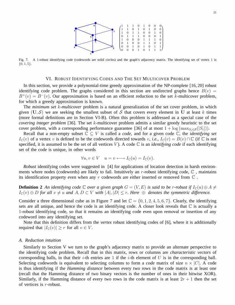
Fig. 7. A 1-robust identifying code (codewords are solid circles) andthe graph’s adjacency matrix. The identifying set of vertex1 is{0, 1, 5}.
VI. ROBUST IDENTIFYING CODES AND THE SET MULTICOVER PROBLEM
In this section, we provide a polynomial-time greedy approximation of the NP-complete [16, 20] robustidentifying code problem. The graphs considered in this section are undirected graphs henceB(v) =B+(v) = B−(v). Our approximation is based on an efficient reduction to the set k-multicover problem,for which a greedy approximation is known.
The minimum setk-multicoverproblem is a natural generalization of the set cover problem, in whichgiven (U,S) we are seeking the smallest subset ofS that covers every element inU at leastk times(more formal definitions are in Section VI-B). Often this problem is addressed as a special case of thecovering integer problem[36]. The setk-multicover problem admits a similar greedy heuristic to the setcover problem, with a corresponding performance guarantee[36] of at most1 + log (maxSi∈S(|Si|)).
Recall that a non-empty subsetC ⊆ V is called acode, and for a given codeC, the identifying setIC(v) of a vertexv is defined to be the codewords directed towardsv, i.e., IC(v) = B(v)∩C (if C is notspecified, it is assumed to be the set of all verticesV ). A codeC is an identifying codeif each identifyingset of the code is unique, in other words
∀u, v ∈ V u = v ←→ IC(u) = IC(v).
Robustidentifying codes were suggested in [4] for applications oflocation detection in harsh environ-ments where nodes (codewords) are likely to fail. Intuitively an r-robust identifying code,C , maintainsits identification property even when anyr codewords are either inserted or removed fromC .
Definition 2 An identifying codeC over a given graphG = (V,E) is said to ber-robust if IC(u)⊕A 6=IC(v)⊕D for all v 6= u and A, D ⊂ V with |A|, |D| ≤ r. Here ⊕ denotes the symmetric difference.
Consider a three dimensional cube as in Figure 7 and letC = {0, 1, 2, 4, 5, 6, 7}. Clearly, the identifyingsets are all unique, and hence the code is an identifying code. A closer look reveals thatC is actually a1-robust identifying code, so that it remains an identifyingcode even upon removal or insertion of anycodeword into any identifying set.
Note that this definition differs from thevertexrobust identifying codes of [6], where it is additionallyrequired that|IC(v)| ≥ r for all v ∈ V .
A. Reduction intuition
Similarly to Section V we turn to the graph’s adjacency matrix to provide an alternate perspective tothe identifying code problem. Recall that in this matrix, rows or columns arecharacteristic vectorsofcorresponding balls, in that theiri-th entries are1 if the i-th element ofU is in the corresponding ball.Selecting codewords is equivalent to selecting columns to form a codematrix of sizen × |C|. A codeis thus identifying if theHamming distancebetween every two rows in the code matrix is at least one(recall that the Hamming distance of two binary vectors is the number of ones in their bitwise XOR).Similarly, if the Hamming distance of every two rows in the code matrix is at least2r + 1 then the setof vertices isr-robust.

22
We next form then(n−1)2× n differencematrix by stacking the bitwise XOR results of every two
different rows in the adjacency matrix. The problem of finding a minimum sizer-robust identifying codeis equivalent to selecting a minimum number of columns to form a code matrix for which the Hammingdistance between any pair of distinct rows is at least2r + 1. Or equivalently: selecting the minimumnumber of columns in the difference matrix such that all rowsin the resulting matrix have Hammingweight of at least2r + 1. This equivalent problem is nothing but a set(2r + 1)-multicover problem, ifone regards the columns of the difference matrix as the characteristic vectors of a family of subsetsSover the base set of all pairs of rows in the adjacency matrix.
In the next subsection we formalize this intuition into a rigorous reduction.
B. Reduction
In this section, we formally reduce the problem of finding thesmallest sizedr-robust identifying codeover an arbitrary graphG to a (2r + 1)-multicover problem.
Formally we connect the following problems:c) SET MULTI-COVER (SCk):
INSTANCE: SubsetsS of U , an integerk ≥ 1.SOLUTION: S′ ⊆ S such that for every element u ∈ U , |{s ∈ S ′ : u ∈ s}| ≥ k.MEASURE: The size of the multicover:|S′|.
d) Robust ID-CODE (rID):INSTANCE: GraphG = (V, E), and integerr ≥ 0.SOLUTION: An r-robust identifying codeC ⊆ V .MEASURE: The size|C|.
Theorem 5 Given a graphG of n vertices, finding anr-robust identifying code requires no morecomputations than a(2r + 1)-multicover solution over a base set ofn(n−1)
2elements together withO(n3)
operations of lengthn binary vectors.
Recall that thedifference setDC(u, v) is the symmetric difference between the identifying sets ofverticesu, v ∈ V . In addition, recall that thedistinguishing setδc is the set of vertex pairs inU for whichc is a member of their difference set whereU = {(u, z)|u 6= z ∈ V }.
As indicated in [4], a code isr-robust if and only if the size of the smallest difference setis at least2r + 1. Equivalently, a code isr-robust if and only if its distinguishing sets(2r + 1)-multicover all thepairs of vertices in the graph.
Lemma 7 GivenG = (V,E) the following statements are equivalent:1) C = {c1, ..., ck} is an r-robust identifying code.2) |DC(u, v)| ≥ 2r + 1, for all u 6= v ∈ V3) The set{δc1 , ..., δck
} forms a(2r + 1)-multicover ofU = {(u, v) | ∀ u 6= v ∈ V }.
Proof of Theorem 5: Let SMC be a set multicover algorithm and consider the following constructionof an r-robust identifying code.
rID(G, r)→ C
1. Compute{I(u)|u ∈ V }.2. Compute∆ = {δu|u ∈ V }.3. C← SMC(2r + 1,U ,∆)4. OutputC← {u ∈ V |δu ∈ C}
The resulting code,C, is guaranteed by Lemma 7 to be anr-robust identifying code, and the optimalityof the set cover in step 3 guarantees that no smaller identifying code can be found. To complete the proofwe observe that computing the identifying setsI(u) naively requiresΘ(n2) additions of binary vectors,and computing∆ requiresn operations for each of then(n−1)
2elements inU .

23
Algorithm 2 Greedy robust ID-coderID− GREEDY
Let G = (V,E) be a given graph, and letSMC− GREEDY(k,U,S) be the greedy set multicover algorithm,then given integerr the r-robust identifying code greedy algorithm is:rID− GREEDY(G, r)→ Cgreedy
1) Compute{I(u)|u ∈ V }.2) Compute∆ = {δu|u ∈ V }.3) C← SMC− GREEDY(2r + 1,U ,∆)4) OutputCgreedy ← {u ∈ V |δu ∈ C}
C. Approximation algorithm
The set multicover problem admits a greedy solution: in eachiteration select the set which covers themaximum number of nonk-multicovered elements. We use this heuristic together with Theorem 5 tointroduce anr-robust identifying code algorithm (Algorithm 2).
It is well known [36] that the performance guarantee of the heuristic of the set multicover problem(defined as the ratio of the sizes of the greedy and minimum multicovers) is upper bounded by1 + lnα,whereα is the largest set’s size, namely
|SMC− GREEDY(k,U,S)|
|SMC(k,U,S)|≤ 1 + lnα (9)
for any set multicover problem(k,U,S).
Theorem 6 Given a graphG = (V, E), ofn nodes, letcgreedy, cmin be the sizes of the greedy (rID− GREEDY)and minimumr-robust identifying codes, respectively, then
cgreedy
cmin≤ 1 + log n + log bmax
wherebmax is the ball’s size closest ton2
Proof: δv contains all pairs of vertices, whichv appear exactly in one of their incoming balls. Thereforev distinguishes between all pairs having one vertex inv’s outgoing ball,B(v), and the second fromV − B(v). Hence the size of a distinguishing set is given by|δv| = |B(v)| (n− |B(v)|). It is easy tosee that the vertex with the largest distinguishing set is the one whose outgoing ball size is closest ton
2.
Denote this outgoing ball bybmax, and based on Theorem 5 andrID− GREEDY algorithm plug the sizeof its distinguishing set into the bound of Equation (9) to get
cgreedy
cmin≤ 1 + log(n− bmax) + log bmax
< 1 + log n + log bmax.
D. Localized robust identifying code and its approximation
It was observed in [4, 5] that anr-robust identifying code can be built in a localized manner,where eachvertex only considers its two-hop neighborhood. This localization is possible when the identifying codesare required to produce only non-empty identifying sets5. In this section and henceforth we introduce thisrequirement, and call the resulting codes -localized identifying codes. These codes and their approximationalgorithm are critical to the development of the distributed algorithms of the next section. Note that bydefinition the localized identifying codes are also dominating sets.
5In fact this definition of identifying codes is the traditional definition (e.g., [1])

24
Algorithm 3 Localizedr-robust coderID− LOCAL(r, G)
We start with a graphG = (V, E) and a non-negative integerr. The greedy set multicover approximationis denotedSMC− GREEDY(k,U,S).
1) Compute{D(u, v)|u ∈ V, v ∈ B(u; 2)}2) Compute∆2 = {δ2
u|u ∈ V }.3) C←SMC− GREEDY(2r + 1,U 2, ∆2)4) OutputClocal ← {u ∈ V |δ2
u ∈ C}
Let G = (V,E) be an undirected graph; we define the distance metricρ(u, v) to be the number of edgesalong the shortest path from vertexu to v. The ball of radiusl aroundv is denotedB(v; l) and definedto be {w ∈ V |ρ(w, v) ≤ l}. So far we encountered balls of radiusl = 1, which we simply denoted byB(v).
Recall that a vertex cover (or dominating set) is a set of vertices, such that the union of their ballsof radius 1 coversV . We further extend this notion and define anr-dominatingset as a set of vertices,which r-multicoversV (these sets are closely related toµ-fold 1-covering codes [42]).
Note that the definition of difference sets and hence identifying codes still involves only radius oneballs, unlike the radius(l > 1) identifying codes discussed in [1].
Lemma 8 Given a graphG = (V, E), an (r + 1)-dominating setC is also anr-robust identifying codeif and only if |DC(u, v)| ≥ 2r + 1 for all u, v ∈ V such thatρ(u, v) ≤ 2.
Proof: The forward implication is an application of Lemma 7. For thereverse implication we takeCto be anr +1 dominating set and assume that|DC(u, v)| ≥ 2r +1 for ρ(u, v) ≤ 2; we will show that thisassumption is also valid forρ(u, v) > 2. This is because, forρ(u, v) > 2, we have thatB(v)∩B(u) = ∅,meaning that|DC(u, v)| = |B(v) ∩ C|+ |B(u) ∩C|. SinceC is anr + 1 dominating set, it must be that|B(y) ∩ C| ≥ r + 1 for all verticesy, giving that |DC(u, v)| > 2r + 1. Applying Lemma 7 we thus seethat C must ber-robust.
The localized robust identifying code approximation Lemma 8 can serve as the basis for a reductionfrom an identifying code problem to a set cover problem, similar to the one in Theorem 5. The maindifference is that we will restrict base elements to vertex pairs that are at most two hops apart, and wethen need to guarantee that the resulting code is stillr-robust.
Towards this end we defineU 2 = {(u, v) | ρ(u, v) ≤ 2}, the set of all pairs of vertices (including(v, v))that are at most two hops apart. Similarly, we will localize the distinguishing setδv to U
2 as follows:
δ2v = (δv ∩ U
2) ∪ {(u, u)|u ∈ B(v)},
The resultinglocalized identifying code approximationis thus given by Algorithm 3 and can be shownto provide anr-robust identifying code for any graph that admits one (we omit the proof due to spaceconsiderations).
Theorem 7 Given an undirected graphG = (V, E) of n vertices, the performance ratiorID− LOCAL isupper bounded by: cgreedy
cmin< ln γ + 1,
whereγ = maxv∈V |B(v)|(|B(v; 3)| − |B(v)|+ 1).
Proof: Recall thatδv includes all vertex pairs where one vertex is in the outgoingball of v and the otheris not. The size of the intersection ofδv and U
2 can be upper bounded by|B(v)|(|B(v; 3)| − |B(v)|),which becomes an equality when all vertices inB(v; 3) are within distance 2 of each other. Finally,

25
δ2v includes also|B(v)| pairs of the same vertex(u, u). Therefore|δ2
v | ≤ |B(v)|(|B(v; 3)| − |B(v)|+ 1),which at its maximum, can be applied to the performance guarantee of Equation (9) to complete the proof.
In the next subsection we present a distributed implementation of the identifying code localized ap-proximation. The following lemma supplements Lemma 8 by providing additional “localization”. At theheart of this lemma lies the fact that each codeword distinguishes between its neighbors and the remainingvertices.
Lemma 9 The distinguishing setsδ2v and δ2
u are disjoint for every pair(u, v) with ρ(u, v) > 4.
Proof: Clearly, δ2v includes all vertex pairs(x, y) ∈ U
2 wherex is a neighbor ofv andy is not. Moreprecisely,(x, y) ∈ δ2
v ifx ∈ B(v) andy ∈ B(x; 2)− B(v). (10)
Moreover, for all such(x, y), ρ(x, v) ≤ 1 and ρ(y, v) ≤ 3. On the other hand, for(x′, y′) ∈ δ2u with
ρ(u, v) > 4, eitherx′ or y′ must be a neighbor ofu, and hence of distance> 3 from v. Thus,δ2u andδ2
v
are disjoint.
Lemma 9 implies that when applying the greedy algorithm, a decision on choosing a codeword onlyaffects decisions on vertices within four hops; the algorithm is thus localized to vicinities of balls ofradius four.
VII. D ISTRIBUTED APPROXIMATION TO ROBUST IDENTIFYING CODES
Several parallel algorithms exist in the literature for setcover and for the more general covering integerprograms (e.g., [35]). There are also numerous distributed algorithms for finding a minimum (connected)dominating set based on set cover and other well known approximations such as linear programmingrelaxation (e.g., [43]). In a recent work, Kuhn et al. [44] devised a distributed algorithm for finding adominating set with a constant runtime. The distributed algorithm uses a design parameter which providesa tradeoff between the runtime and performance.
Unfortunately, the fundamental assumption of these algorithms is that the elements of the base set areindependent computational entities (i.e., the nodes in the network); this makes it non-trivial to applythemin our case, where elements correspond to pairs of nodes thatcan be several hops apart. Moreover, weassume that the nodes are energy constrained so that reducing communications is very desirable, even atthe expense of longer execution times and reduced performance.
We next provide two distributed algorithms. The first is completely asynchronous, guarantees a perfor-mance ratio of at mostln γ + 1, and requiresΘ(cdist) iterations at worst, wherecdist is the size of theidentifying code returned by the distributed algorithm andγ = maxv∈V |B(v)|(|B(v; 3)| − |B(v)| + 1|).The second is a randomized algorithm, which requires a coarse synchronization, guarantees a performance
ratio of at mostln γ + 1, and for some arbitrarily smallǫ > 0 operates withinO
(
γnK+2+ǫ
K−1
K
)
time slots
(resulting in O(cdistmaxv∈V |B(v; 4|)) messages). The valueK ≥ 2 is a design parameter that tradesbetween the size of the resultingr-robust identifying code and the required number of time slots tocomplete the procedure.
In the next subsection we describe the model and initialization stages that are common to both distributedalgorithms.
A. Model and initialization
With a model similar to [4], we assume that every vertex (node) in a graph is an independent processingentity that is pre-assigned a unique serial number and can communicate reliably and collision-freely
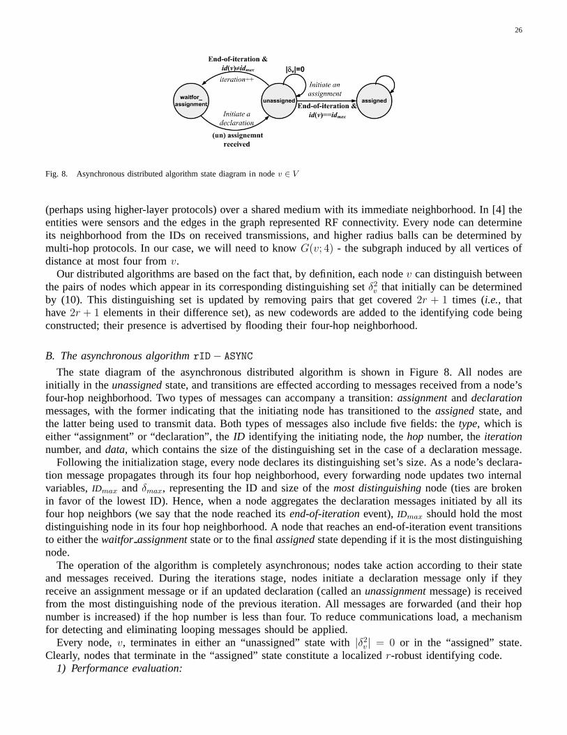
26
Fig. 8. Asynchronous distributed algorithm state diagram in nodev ∈ V
(perhaps using higher-layer protocols) over a shared medium with its immediate neighborhood. In [4] theentities were sensors and the edges in the graph representedRF connectivity. Every node can determineits neighborhood from the IDs on received transmissions, and higher radius balls can be determined bymulti-hop protocols. In our case, we will need to knowG(v; 4) - the subgraph induced by all vertices ofdistance at most four fromv.
Our distributed algorithms are based on the fact that, by definition, each nodev can distinguish betweenthe pairs of nodes which appear in its corresponding distinguishing setδ2
v that initially can be determinedby (10). This distinguishing set is updated by removing pairs that get covered2r + 1 times (i.e., thathave2r + 1 elements in their difference set), as new codewords are added to the identifying code beingconstructed; their presence is advertised by flooding theirfour-hop neighborhood.
B. The asynchronous algorithmrID− ASYNC
The state diagram of the asynchronous distributed algorithm is shown in Figure 8. All nodes areinitially in the unassignedstate, and transitions are effected according to messages received from a node’sfour-hop neighborhood. Two types of messages can accompanya transition:assignmentanddeclarationmessages, with the former indicating that the initiating node has transitioned to theassignedstate, andthe latter being used to transmit data. Both types of messages also include five fields: thetype, which iseither “assignment” or “declaration”, theID identifying the initiating node, thehop number, theiterationnumber, anddata, which contains the size of the distinguishing set in the case of a declaration message.
Following the initialization stage, every node declares its distinguishing set’s size. As a node’s declara-tion message propagates through its four hop neighborhood,every forwarding node updates two internalvariables,IDmax andδmax, representing the ID and size of themost distinguishingnode (ties are brokenin favor of the lowest ID). Hence, when a node aggregates the declaration messages initiated by all itsfour hop neighbors (we say that the node reached itsend-of-iterationevent),IDmax should hold the mostdistinguishing node in its four hop neighborhood. A node that reaches an end-of-iteration event transitionsto either thewaitfor assignmentstate or to the finalassignedstate depending if it is the most distinguishingnode.
The operation of the algorithm is completely asynchronous;nodes take action according to their stateand messages received. During the iterations stage, nodes initiate a declaration message only if theyreceive an assignment message or if an updated declaration (called anunassignmentmessage) is receivedfrom the most distinguishing node of the previous iteration. All messages are forwarded (and their hopnumber is increased) if the hop number is less than four. To reduce communications load, a mechanismfor detecting and eliminating looping messages should be applied.
Every node,v, terminates in either an “unassigned” state with|δ2v | = 0 or in the “assigned” state.
Clearly, nodes that terminate in the “assigned” state constitute a localizedr-robust identifying code.1) Performance evaluation:

27
Algorithm 4 Asynchronousr-robust algorithm (rID− ASYNC)We start with a graphG, with vertices labeled byID, and a non-negative integerr. The following distributedalgorithm run at nodev ∈ V produces anr-robust identifying code.PRECOMP:
• Computeδ2v using (10).
• Initiate a declaration message and set state = “unassigned”.• Set IDmax = ID(v), δmax = |δ2
v |, andms to be an empty assignment message.ITERATION:
• Incrementhop(ms) and forward all messages ofhop(ms) < 4.• if received an assignment messagems with state 6= assigned then
– Updateδ2v by removing all pairs covered2r + 1 times.
– Initiate a declaration message and set state = “unassigned”.– Reinitialize IDmax = ID(v) andδmax = |δ2
v |.• if state = waitfor assignment and received anun-assignmentmessage then initiate a declaration
message.• if received a declaration messagems with state 6= assigned then
– if δmax < data(ms) or (δmax = data(ms) andIDmax > ID(ms)) thenδmax = data(ms), IDmax =ID(ms)
• if end-of-iterationreached then,– if IDmax = ID(v) and |δ2
v | > 0 thenstate = assigned, initiate an assignment message.– otherwisestate = waitfor assignment.
1
2
3
|V|
Fig. 9. Worst case topology for the asynchronous distributed r-robust algorithm in terms of runtime.
Theorem 8 Algorithm 4 (rID− ASYNC) requiresΘ(cdist) iterations and has a performance ratio
cdistcmin
< ln γ + 1,
whereγ = maxv∈V |B(v)|(|B(v; 3)| − |B(v)|+ 1|).
The first part of the Theorem follows from Theorem 7 and the fact that only the most distinguishingsets in a four hop neighborhoods is assigned to be a codeword.To see the number of iterations of thealgorithm, we first note that in each iteration at least one codeword is assigned. The case of a cycle graph(Fig. 9) demonstrates that, in the worst case, exactly one node is assigned per iteration.
It follows that the amount of communications required in theiteration stage isΘ(cdist|V |max(|B(v; 4)|)),which can be a significant load for a battery powered sensor network. This can be significantly reduced ifsome level of synchronization among the nodes is allowed. Inthe next section we suggest a synchronizeddistributed algorithm that eliminates declaration messages altogether.
28
Algorithm 5 Synchronousr-robust algorithm (rID− SYNC)We start with a graphG and non-negative integerr. The following distributed algorithm run at nodev ∈ V produces anr-robust identifying code.PRECOMP:
• Set:slot = sF , subslot = L, state = unassigned.• Calculate the assignment slot.
ITERATE: while state = unassigned andslot ≥ s1 do,• l = random{1, ..., L}• if received assignment message,ms then,
– if hop(ms) < 4 forward ms with hop(ms) + +.– Recalculate the assignment slot.
• else if subslot = l andslot = as then,– state = assigned– Transmitms with id(ms) = id(v), andhop(ms) = 1
C. A low-communications randomized algorithmrID− SYNC
In this subsection, we assume that a coarse time synchronization among vertices within a neighborhoodof radius four can be achieved. In particular, we will assumethat the vertices maintain a basic timeslot, which is divided intoL subslots. Each subslot duration is longer than the time required for afourhop one-way communication together with synchronization uncertainty and local clock drift. After aninitialization phase, the distributed algorithm operateson a timeframe, which consists ofF slots arrangedin decreasing fashion fromsF to s1. In general,F should be at least as large as the largest distinguishingset (e.g.,F = n(n−1)
2will always work). A frame synchronization within a neighborhood of radius four
completes the initialization stage.The frame synchronization enables us to eliminate all the declaration messages of the asynchronous
algorithm. Recall that the declaration messages were required to perform two tasks: (i) determine themost distinguishing node in its four hop neighborhood, and (ii) form an iteration boundary,i.e., end-of-iteration event. The second task is naturally fulfilled by maintaining the slot synchronization. The first taskis performed using the frame synchronization: every node maintains a synchronized slot counter, whichcorresponds to the size of the currentmost distinguishingnode. If the slot counter reaches the size of anode’s distinguishing set, the node assigns itself to the code. The subslots are used to randomly breakties.
1) Iterations stage:Each iteration takes place in one time slot, starting from slot sF . During a slotperiod, a node may transmit a messagems indicating that it is assigning itself as a codeword; the messagewill have two fields: the identification number of the initiating node,id(ms), and the hop number,hop(ms).A node assigns itself to be a codeword if itsassignment time, which refers to a slotas and subslotl, hasbeen reached. Every time an assignment message is received,the assignment slotas of a node is updatedto match the size of its distinguishing set; the assignment subslot is determined randomly and uniformlyat the beginning of every slot.
2) Performance evaluation:Algorithm 5 (rID− SYNC) requires at mostO(n2) slots (O(Ln2) subslots),though it can be reduced toO(Lγ) if the maximum size of a distinguishing set is propagated throughout thenetwork in the precomputation phase. The communications load is low (i.e.,O(cdist·maxv∈V (|B(v; 4)|))),and includes only assignment messages, which are propagated to four hop neighborhoods.
In the case of ties,rID− SYNC can provide a larger code than gained from the localized approximation.This is because ties in the distributed algorithm are brokenarbitrarily, and there is a positive probability(shrinking as the number of subslotsL increases) that more than one node will choose the same subslotwithin a four hop neighborhood. As such,L is a design parameter that provides a tradeoff between
29
performance ratio guarantees and the runtime of the algorithm as suggested in the following theorem.
Theorem 9 For asymptotically large graphs, AlgorithmrID− SYNC guarantees with high probability aperformance ratio of
cdistcmin
< K(ln γ + 1),
whereγ = maxv∈V |B(v)|(|B(v; 3)| − |B(v)| + 1|). The algorithm also requiresO
(
γnK+2+ǫ
K−1
K
)
subslots
to complete for design parameterK ≥ 2 and arbitrarily small ǫ > 0.
Proof: If no more thanK tied nodes assign themselves simultaneously on every assignment slot,then we can upper bound the performance ratio by a factorK of the bound in Theorem 7, as in thetheorem statement. We next determine the number of subslotsL needed to guarantee the above assumptionasymptotically with high probability.
Let P (K) denote the probability that no more thanK tied nodes assign themselves in every assignmentslot. Clearly,P (K) ≥ (1 − p(K))
cdist, where p(K) is the probability that, whent nodes are assignedindependently and uniformly toL subslots, there are at leastK < t assignments to the same subslot. Onecan see that
p(K) =t∑
k=K
L
(
t
k
)
L−k
(
1−1
L
)t−k
≤t∑
k=K
(
t
k
)
L1−k ≤t∑
k=K
L
(
te
Lk
)k
≤ tL
(
te
LK
)K
,
for e being the natural logarithm and based on the assumption thatteLK
< 1. Let t = cdist = n (this only
loosens the bound) andL = eK
nK+2+ǫ
K−1 . Then,
P (K) ≥
(
1− tL
(
te
LK
)K)cdist
≥
(
1−e
K
1
n1+ǫ
)n
→ 1.
VIII. S IMULATIONS
Here we have simulated the centralized, localized and synchronized distributed identifying code algo-rithms, and applied them to grids (e.g., [6]), random graphs with different edge probabilities [14], andto geometric random graphs with different nodes densities [31]. As a performance measure, we use theaveraged size of the identifying code. For the case ofr = 0 (i.e., simple identifying code) the simulationresults are compared to the algorithm suggested by Ray et al.in [4]. In addition, we show a combinatoriallower bound derived first by Karpovsky et al. in [1], and the asymptotic result (inn - the size of thegraph) of Moncel et al. [14], who showed that an arbitrary setof a threshold number of codewords is anidentifying code with high probability, and that this number is asymptotically tight.

30
1− robustidentifyingCode
IdentifyingCode
Fig. 10. Examples of efficient constructions of identifyingtiles for the square, king and triangular infinite grids produced by the localized,rID− LOCAL (triangles), and centralized,rID− GREEDY (circles), algorithms. The constructions densities can befound in Table I.
A. Infinite grids
Significant amount of the study efforts into identifying codes were focused on infinite grids [1, 6].Many of these studies use tilings to suggest constructive upper bounds on the size of an identifyingcodes. Table I compares these tight constructions and bounds with the best outcomes of the centralized,localized and the distributed algorithms when applied to the square, king, and triangle infinite grids.Infinite grids were emulated by the use of finite girds with wrapped around edges (torii). The size ofthe torus limits the size of the largest tile of the infinite code, and therefore has a large impact on theresulting codes. The algorithms outcomes were also varied by randomly relabeling the torus nodes inbetween runs. Table I summarizes the best results achieved for the different torii sizes, and their matchingconstructions appear in Figure 10. Surprisingly, the localized (rID− LOCAL) algorithm outperformed thecentralized (rID− GREEDY) for almost all grids and torii sizes, coming pretty close tothe results in [6].One reason for this behavior may be that the additional requirement that the code will also be dominatingis not significant when it comes to grids. Therefore the centralized algorithm takes into account manyirrelevant vertices pairs that may influence the optimization step.
Finally, Figure 11 shows that it is sometimes possible to getvery good codes for small graphs througha pruned exhaustive search (in this case, an adaptation of the branch-and-bound algorithm [45]). The 1-robust identifying codes in the figure for the hexagonal and triangular finite grids actually have a densityslightly better than those reported in [6].
B. (Geometric) random graphs
Fig. 12(a) shows the theoretic lower bound and the results ofthe centralized greedy algorithm. It can beseen that a significant enhancement in performance over the algorithm devised by Ray et al. is achieved.It should be noted that asn grows the curves for basically any algorithm should converge to Moncel’s

31
Density: 52/64 Density=21/36
Fig. 11. Branch and bound algorithm results for 1-robust identifying codes for the hexagonal (left) and triangular (right) grids. The redcircles represent codewords, and the tile is captured by a gray square.
TABLE I
DENSITIES OF IDENTIFYING CODES FOR INFINITE GRIDS TAKEN FROM[6] VS. SIMULATION RESULTS USING OUR APPROXIMATIONS(IN
BRACKETS).
square king triangular
ID code 112
320(115
320) 16
72( 17
72) 27
108( 32
108)
1-Robust ≤ 40
64( 43
64) 32
64( 35
64) ≤ 24
40(25
40)
asymptotic result, as illustrated in Fig. 13(a). Still, theconvergence rate appears to be very slow, suggestingthat for reasonably large networks there is a lot to gain fromthe suggested algorithms compared to thesimple approach of arbitrarily picking a code, whose size satisfies the threshold number of [14].
Fig. 12(b) shows the simulation results for the localized and distributed algorithms compared to thecentralized one. Recall that the performance of the asynchronous algorithm,rID− ASYNC, is identical tothe localized approximation. It can be observed that the results of the localized algorithm nearly matchthe results of the centralized algorithms. Divergence is evident for low edge probabilities, where it isharder to find a dominating set. Recall that there is a tradeoff between performance and the runtime ofthe synchronized distributed algorithm,rID− SYNC. The smaller the number of subslots parameter,L,the shorter the runtime and the larger the degradation in performance due to unresolved ties. Degradationin performance is also more evident when ties are more likelyto happen,i.e., when the edge probabilityis approaching0.5. The results of the centralized r-robust identifying code algorithm are shown inFigure 12(c).
Fig. 13(b) shows the codeword density for geometric random graphs using the localized and distributedapproaches, and the fraction of such graphs admitting an identifying code. It also presents the largestfraction of indistinguishablenodes,i.e., nodes that share the same identifying set, obtained in the simu-lation. As can be seen, the localized and distributed approaches (withL = 10) yield very similar codesizes. The fraction of graphs admitting identifying codes is rather small (less than half the graphs) evenfor high node densities. However, the size of indistinguishable nodes sets is still small, suggesting thatthe system’s reduction inresolution, i.e. the geometric size of the largest indistinguishable set, is not too

32
0.1 0.2 0.3 0.4 0.5 0.6 0.7 0.8 0.95
10
15
20
25
30n=128 random graph
Edge probability
Ave
rage
ID c
ode
size
Lower bound (Karpovsky et. al.)
Ray et. al.Centralized
(a) Centralized greedy algorithm
0.1 0.2 0.3 0.4 0.5 0.6 0.7 0.8 0.98
10
12
14
16
18
20
22
24
26n=128 random graph
Edge probability
Ave
rage
ID c
ode
size
Centralized
Distributed
Localized
L=5
L=10
L=20
(b) Localized (and rID− ASYNC) and distributed algorithm,rID− SYNC, for different subslot (L) values
0.1 0.2 0.3 0.4 0.5 0.6 0.7 0.8 0.90
10
20
30
40
50
60
70
n=128 random graph
Edge probability
Ave
rage
gre
edy
ID c
ode
size
r=1
r=0 (IDcode)
r=2
r=7
(c) Centralizedr-robust identifying codes algorithm.
Fig. 12. Average size of the minimum identifying code for random graphs with edge probabilityp, andn = 128 vertices.
high. It should be noted that approaches such that of ID-CODE[4] are not designed to cope with graphswhich do not have identifying codes, resulting in a code of all vertices.
IX. CONCLUSIONS
We have provided connections between identifying codes problems and covering problems, for whichgreedy approximation algorithms are known. The connections to traditional identifying codes have beensufficiently size-preserving to produce an approximation algorithm, and should be useful for the numberof identifying code applications that have been developed in the literature. In addition, we have providedgeneral hardness of approximation results that show that our approximations are very close to the bestpossible. In particular, for the case of (non robust) identifying codes we show that a known approximationachieves up to a small constant multiple of the best possibleperformance achievable by any polynomialapproximation (under commonly used complexity assumptions). It remains an open question if ourapproximation algorithms for the(r ≥ 1)-robust identifying codes are similarly near-optimal.
We have also demonstrated by simulations that the proposed algorithms outperform the existing ap-proximation algorithm of [4] and that they come close to efficient combinatorial constructions of robustidentifying codes for two dimensional grids, which have been well-studied in the literature. We havefurther provided two flavors of distributed algorithms thatmay be used for practical implementations innetwork applications.

33
32 64 128 256 3842
3
4
5
6
7
8
9
10
11
Number of nodes (n)
|C|/l
og(n
)
Normailized average size of the identifying code (r=0) for random graphs with edge probability p=0.1.
Moncel et alAssymptotic bound
Ray et al
Centralized
Karpovsky et alLower bound
(a) Average size of the simple (r = 0) identifying code forrandom graphs with edge probabilityp = 0.1, and differentnumber of vertices.
0 20 40 60 80 100 120 1400
0.1
0.2
0.3
0.4
0.5
nodes density
GRG with different nodes densities
Distributed (L=10) codewords density
Localized approx.codewords density
precentage of identifying codes
Largest normailized number ofundestinguishable nodes
(b) Normalized size of the code for the localized (andrID− ASYNC) and distributedrID− SYNC algorithm, fractionof graphs admitting an identifying code, and maximum frac-tion of indistinguishable nodes for geometric random graphswith different node densities.
Fig. 13. Additional simulation results for (geometric) random graphs.
ACKNOWLEDGMENT
The anonymous reviewers at the IEEE Transactions on Information Theory have provided thorough andsignificant improvements that have been incorporated into this paper.
REFERENCES
[1] M. G. Karpovsky, K. Chakrabarty, and L. B. Levitin, “A newclass of codes for identification of vertices in graphs,”IEEE Transactionson Information Theory, vol. 44, no. 2, pp. 599–611, March 1998.
[2] S. Ray, R. Ungrangsi, F. D. Pellegrinin, A. Trachtenberg, and D. Starobinski, “Robust location detection in emergency sensor networks,”Proceedings INFOCOM, April 2003.
[3] R. Ungrangsi, A. Trachtenberg, and D. Starobinski, “An implementation of indoor location detection systems based on identifyingcodes,”Proceedings of the IFIP International Conference on Intelligence in Communication Systems (INTELLCOMM 04), 2004.
[4] S. Ray, D. Starobinski, A. Trachtenberg, and R. Ungrangsi, “Robust location detection with sensor networks,”IEEE Journal on SelectedAreas in Communications (Special Issue on Fundamental Performance Limits of Wireless Sensor Networks), vol. 22, no. 6, August2004.
[5] M. Laifenfeld and A. Trachtenberg, “Disjoint identifying codes for arbitrary graphs,”IEEE International Symposium on InformationTheory, Adelaide, Australia, 4-9 Sept 2005.
[6] I. Honkala, M. Karpovsky, and L. Levitin, “On robust and dynamic identifying codes,”IEEE Transactions on Information Theory,vol. 52, no. 2, pp. 599–612, February 2006.
[7] T. Y. Berger-Wolf, W. E. Hart, and J. Saia, “Discrete sensor placement problems in distribution networks,”Journal of Mathematicaland Computer Modelling, vol. 42, no. 13, pp. 1385–1396, Dec 2005.
[8] M. Laifenfeld, A. Trachtenberg, R. Cohen, and D. Starobinski, “Joint monitoring and routing in wireless sensor networks using robustidentifying codes,”IEEE Broadnets 2007, September 2007.
[9] M. Laifenfeld, A. Trachtenberg, and T. Berger-Wolf, “Identifying codes and the set cover problem,”Proceedings of the 44th AnnualAllerton Conference on Communication, Control, and Computing, Sept 2006.
[10] S. Gravier and J. Moncel, “Construction of codes identifying sets of vertices,”The Electronic Journal of Combinatorics, vol. 12, no. 1,2005.
[11] I. Honkala and A. Lobstein, “On identifying codes in binary Hamming spaces,”Journal of Combinatorial Theory, Series A, vol. 99,no. 2, pp. 232–243, 2002.
[12] Y. Ben-Haim and S. Litsyn, “Exact minimum density of codes identifying vertices in the square grid,”SIAM Journal of DiscreteMathematics, vol. 19, no. 1, pp. 69–82, 2005.
[13] S. R. T. Laihonen, “Codes identifying sets of vertices,” Lecture Notes in Computer Science 2227, 2001.[14] J. Moncel, A. Frieze, R. Martin, M. Ruszink, and C. Smyth, “Identifying codes in random networks,”IEEE International Symposium
on Information Theory, Adelaide, 4-9 Sept., 2005.[15] P. Slater, “Fault-tolerant locating-dominating sets,” Discrete Mathematics, vol. 249, pp. 179–189, 2002.[16] I. Charon, O. Hudry, and A. Lobstein, “Identifying and locating-dominating codes: NP-completeness results for directed graphs,”IEEE
Transactions on Information Theory, vol. 48, no. 8, pp. 2192–2200, August 2002.[17] S. Gravier, R. Klasing, and J. Moncel, “Hardness results and approximation algorithms for identifying codes and locating-dominating
codes in graphs,” LaBRI, Technical Report RR-1417-06, November 2006.
34
[18] J. Suomela, “Approximability of identifying codes andlocating–dominating codes,”Information Processing Letters, vol. 103, no. 1,pp. 28–33, 2007.
[19] K. B. Lakshmanan, D. J. Rosenkrantz, and S. S. Ravi, “Alarm placement in systems with fault propagation,”Theoretical ComputerScience, vol. 243, no. 1-2, pp. 269–288, 2000.
[20] I. Charon, O. Hudry, and A. Lobstein, “Minimizing the size of an identifying or locating-dominating code in a graph is NP-hard,”Theoretical Computer Science, vol. 290, no. 3, pp. 2109–2120, 2003.
[21] T. Cormen, C. Leiserson, R. Rivest, and C. Stein,Introduction to Algorithms. MIT Press, 2001.[22] I. Charon, S. Gravier, O. Hudry, A. Lobstein, M. Mollard, and J. Moncel, “A linear algorithm for minimum 1-identifying codes in
oriented trees,”Discrete Applied Mathematics, vol. 154, no. 8, pp. 1246–1253, 2006.[23] G. D. Cohen, I. S. Honkala, A. Lobstein, and G. Zemor, “New bounds for codes identifying vertices in graphs.”Electronic Journal of
Combinatorics, vol. 6, 1999.[24] I. Charon, I. S. Honkala, O. Hudry, and A. Lobstein, “General bounds for identifying codes in some infinite regular graphs.”Electronic
Journal of Combinatorics, vol. 8, no. 1, 2001.[25] I. Charon, O. Hudry, and A. Lobstein, “Identifying codes with small radius in some infinite regular graphs.”Electronic Journal of
Combinatorics, vol. 9, no. 1, 2002.[26] I. Charon, I. S. Honkala, O. Hudry, and A. Lobstein, “Theminimum density of an identifying code in the king lattice.”Discrete
Mathematics, vol. 276, no. 1-3, pp. 95–109, 2004.[27] J. Moncel, “On graphs ofn vertices having an identifying code of cardinality⌈log2(n + 1)⌉,” Discrete Applied Mathematics, vol. 154,
no. 14, pp. 2032–2039, 2006.[28] U. Feige, “A threshold of ln n for approximating set cover,” Journal of the ACM, vol. 45, no. 4, pp. 634–652, 1998.[29] P. Berman, B. DasGupta, and M.-Y. Kao, “Tight approximability results for test set problems in bioinformatics,”Journal of Cmputer
and System Sciences, vol. 71, no. 2, pp. 145–162, 2005.[30] R. Raz and S. Safra, “A sub-constant error-probabilitylow-degree test, and a sub-constant error-probability pcpcharacterization of np,”
in STOC ’97: Proceedings of the twenty-ninth annual ACM Symposium on Theory of Computing. New York, NY, USA: ACM Press,1997, pp. 475–484.
[31] T. Muller and J.-S. Sereni, “Identifying and locating-dominating codes in (random) geometric networks,” 2007, submittedtoCombinatorics, Probability and Computing. ITI Series 2006-323 and KAM-DIMATIA Series 2006-797.
[32] L. Lovasz, “On the ratio of optimal integral and fractional covers,”Discrete Mathematics, vol. 13, pp. 383–390, 1975.[33] D. S. Johnson, “Approximation algorithms for combinatorial problems,”Journal of Computer and System Sciences, vol. 9, pp. 256–278,
1974.[34] P. Slavik, “A tight analysis of the greedy algorithm forset cover,”In Proceedings of the 28th Annual ACM Symposium on Theory of
Computing (Philadelphia, Pa.), pp. 435–439, May 1996.[35] S. Rajagopalan and V. Vazirani, “Primal-dual RNC approximation algorithms for set cover and covering integer programs,” SIAM
Journal on Computing, vol. 28, pp. 525–540, 1998.[36] V. Vazirani, Approximation Algorithms. Springer-Verlag, July 2001.[37] K. M. J. D. Bontridder, B. J. Lageweg, J. K. Lenstra, J. B.Orlin, and L. Stougie, “Branch-and-bound algorithms for the test cover
problem,” inESA ’02: Proceedings of the 10th Annual European Symposium on Algorithms. London, UK: Springer-Verlag, 2002, pp.223–233.
[38] K. M. J. D. Bontridder, B. V. Halldrsson, M. M. Halldrsson, C. A. J. Hurkens, J. K. Lenstra, R. Ravi, and L. Stougie, “Approximationalgorithms for the test cover problem,”Mathematical Programming-B 98, no. 1-3, pp. 477–491, 2003.
[39] M. R. Garey and D. S. Johnson,Computers and Intractability: A Guide to the Theory of NP-Completeness. New York, NY, USA:W. H. Freeman & Co., 1979.
[40] B. M. E. Moret and H. D. Shapiro, “On minimizing a set of tests,” SIAM Journal of Scientific & Statistical Computing., vol. 6, pp.983–1003, 1985.
[41] M. Naor, L. J. Schulman, and A. Srinivasan, “Splitters and near-optimal derandomization,” inIEEE Symposium on Foundations ofComputer Science, 1995, pp. 182–191. [Online]. Available: citeseer.ist.psu.edu/naor95splitters.html
[42] G. Cohen, I. Honkala, S. Litsyn, and A. Lobstein,Covering Codes. Elsevier, 1997.[43] Y. Bartal, J. W. Byers, and D. Raz, “Global optimizationusing local information with applications to flow control,”in IEEE
Symposium on Foundations of Computer Science, 1997, pp. 303–312. [Online]. Available: citeseer.ist.psu.edu/bartal97global.html[44] F. Kuhn and R. Wattenhofer, “Constant-time distributed dominating set approximation,”Proceedings of the 22nd ACM Symposium on
Principles of Distributed Computing (PODC’03), July 2003. [Online]. Available: citeseer.ist.psu.edu/kuhn03constanttime.html[45] M. Laifenfeld, “Coding for network applications: Robust identification and distributed resource allocation,” Ph.D. dissertation, Boston
University, 2007.