1

HSPICE – Highlights and Introductions

Techniques for SI Lecture 12 - 15

HSPICE for SI 2

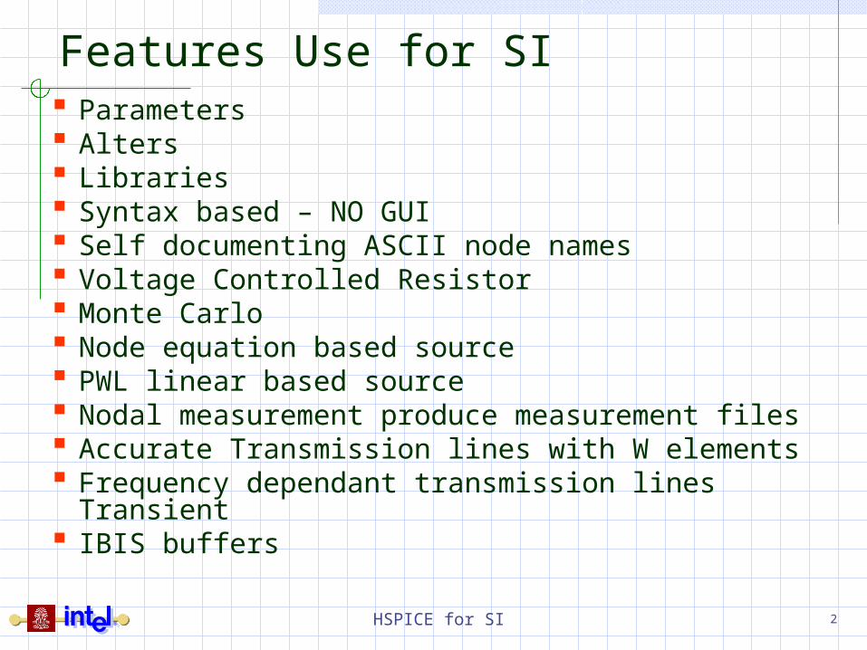
Features Use for SI Parameters Alters Libraries Syntax based – NO GUI Self documenting ASCII node names Voltage Controlled Resistor Monte Carlo Node equation based source PWL linear based source Nodal measurement produce measurement files Accurate Transmission lines with W elements Frequency dependant transmission lines

Transient IBIS buffers

HSPICE for SI 3

Good PracticesModularize with sub-circuits and/or

libraries!Circuit text should flow line a drawing.

Don’t put all caps, resistors, and transmission lines respective separate sections.

Most SI circuits are composed of data generator, buffers, transmission lines, package models, and connectors.

HSPICE for SI 4

Global, Local, and Position Circuit elements within a sub-circuit or the main

net list are position insensitive.Good-news/bad newsIt is easier to follow elements whose code traces out the circuit.

In general parameters are global unless passed into a sub-circuit.

Parameters are not positions insensitiveTreat definition of parameters as last reference wins the definition.This can be trick to determine for complex decks.Deck is old terminology that comes form “punch card decks”

Make the first 8 characters of library names unique

Most HSPICE is case insensitive.The exception is libraries and file names that are enclosed in single quotes

HSPICE for SI 5

Top Level Program First step is to draw as simulation block

diagram. The following slides are a learn by

example method We will review some common HSPICE

elements used for signal integrity

Printed WiringBoard

Buffers

packa

ge

packa

ge

Receiver

Data

genera

tor

HSPICE for SI 6

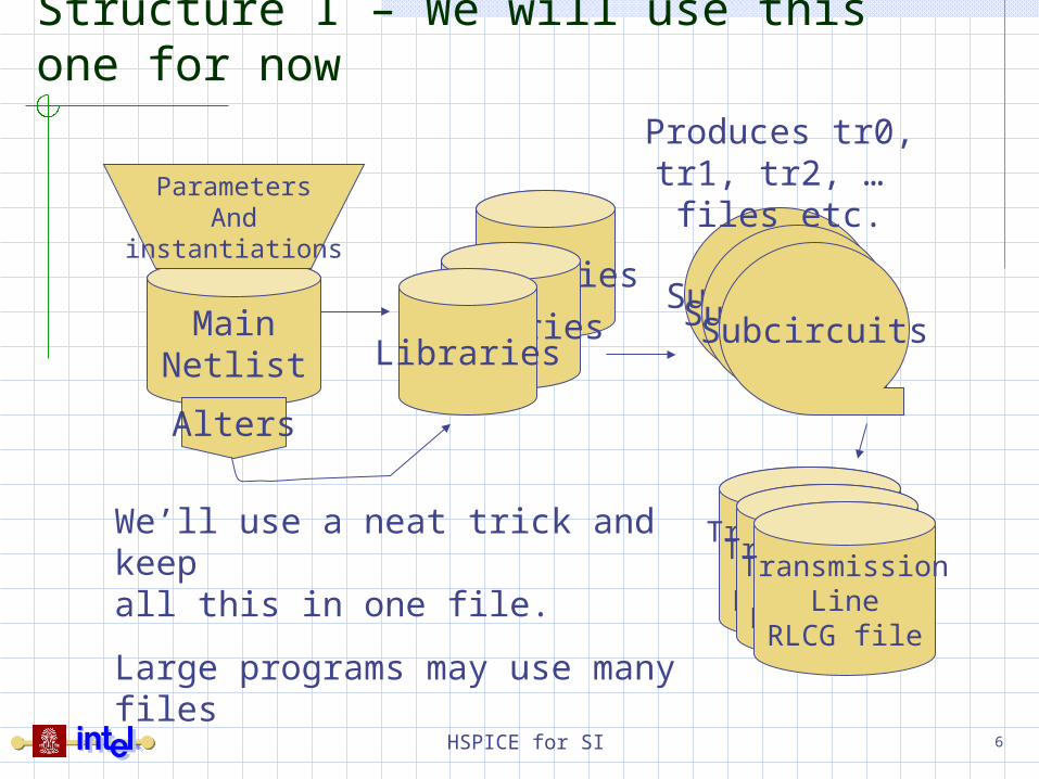
Structure I – We will use this one for now

MainNetlist

Libraries

LibrariesLibraries

SubcircuitsSubcircuitsSubcircuits

We’ll use a neat trick and keep all this in one file.

Large programs may use manyfiles

TransmissionLine

RLCG file

TransmissionLine

RLCG file

TransmissionLine

RLCG file

ParametersAnd

instantiations

Alters

Produces tr0, tr1, tr2, … files etc.

HSPICE for SI 7

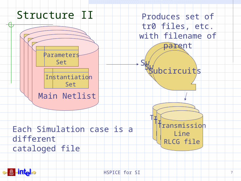
Structure II

SubcircuitsSubcircuitsSubcircuits

Each Simulation case is a differentcataloged file

TransmissionLine

RLCG file

TransmissionLine

RLCG file

TransmissionLine

RLCG file

Main Netlist

ParametersSet

Instantiation Set

Main Netlist

ParametersSet

Instantiation Set

Main Netlist

ParametersSet

Instantiation Set

Main Netlist

ParametersSet

Instantiation Set

Produces set of tr0 files, etc. with

filename of parent

HSPICE for SI 8

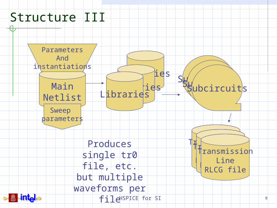
Structure III

MainNetlist

Libraries

LibrariesLibraries

SubcircuitsSubcircuitsSubcircuits

TransmissionLine

RLCG file

TransmissionLine

RLCG file

TransmissionLine

RLCG file

ParametersAnd

instantiations

Sweep parameters

Produces single tr0 file, etc. but

multiple waveforms per

file

HSPICE for SI 9

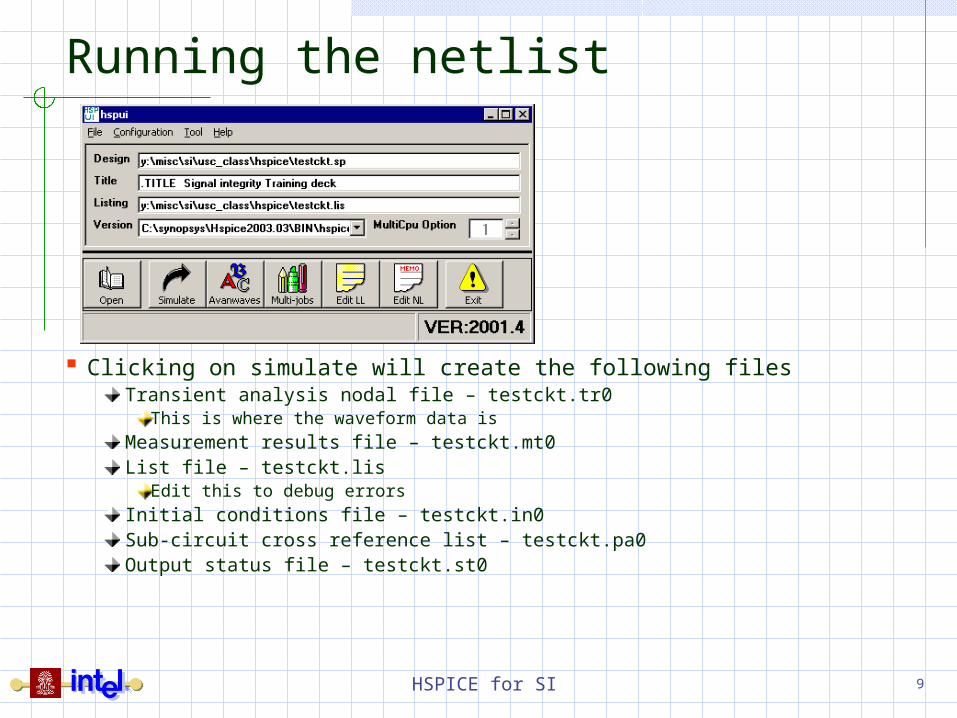
Running the netlist

Clicking on simulate will create the following filesTransient analysis nodal file – testckt.tr0

This is where the waveform data is

Measurement results file – testckt.mt0List file – testckt.lis

Edit this to debug errors

Initial conditions file – testckt.in0Sub-circuit cross reference list – testckt.pa0Output status file – testckt.st0

HSPICE for SI 10

Data Generator

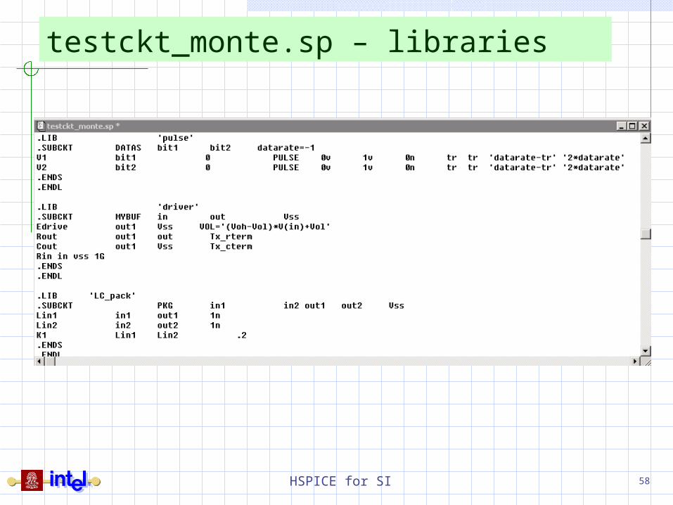
Bit1 and Bit2 are data stream outputs for this sub-circuit “datarate” is passed from the call site

Note that a subcircuit is analogous to a software subroutine”datarate” is set to “-1” to force an error if the parameter was not passed.

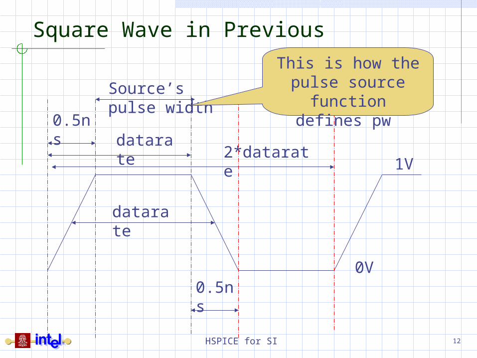
This pulse generator example produces a 1V Aggressor and victim w/ 500 ps rise/fall time.

The pulse width is “datarate” adjusted by the risetime. The period is 2*datarate This special case uses 0v and 1v as a bit stream which has advantages that we will learn later in behavioral modeling.

.LIB 'pulse'

.SUBCKT DATAS bit1 bit2 datarate=-1V1 bit1 0 PULSE 0v 1v 0n 0.5n 0.5n 'datarate- 0.5n' '2*datarate'V2 bit2 0 PULSE 0v 1v 0n 0.5n 0.5n 'datarate- 0.5n' '2*datarate'.ENDS.ENDL

HSPICE for SI 11

Parameterized Generator

We can replace the 0.5n entries with a parameter called tr. (equal rise/fall)

We can set this parameter in the main net list as follows: .PARAM tr=0.5n

Notice the difference between the two parameters tr and datarate

.LIB 'pulse'

.SUBCKT DATAS bit1 bit2 datarate=-1V1 bit1 0 PULSE 0v 1v 0n tr tr 'datarate-tr' '2*datarate'V2 bit2 0 PULSE 0v 1v 0n tr tr 'datarate-tr' '2*datarate'.ENDS.ENDL

HSPICE for SI 12

Square Wave in Previous

0V

1V

0.5ns datarat

e

datarate

2*datarate

0.5ns

Source’spulse width

This is how the pulse source

function defines pw

HSPICE for SI 13

Piece Wise Linear Source

Vol, 0S

bit1, tr*1 bit1, UI*1

bit2,UI*1+tr bit2,UI*2

bit3,UI*2+tr

*rise/fall time = tr

HSPICE for SI 14

AssignmentCreate same driver with a PWL

source and with data pattern “101100110”.

Assume all parameter except datarate are global

Parameterize bits as bit0, bit1, bit2…Parameter for rise and fall time with

a signal parameter TrWrite separate code for parameter

statements in the main netlist.

HSPICE for SI 15

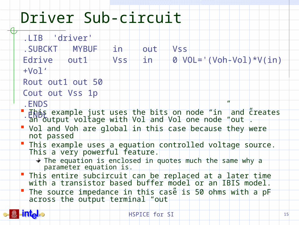
Driver Sub-circuit

This example just uses the bits on node “in” and creates an output voltage with Vol and Vol one node “out”.

Vol and Voh are global in this case because they were not passed

This example uses a equation controlled voltage source. This a very powerful feature.

The equation is enclosed in quotes much the same why a parameter equation is.

This entire subcircuit can be replaced at a later time with a transistor based buffer model or an IBIS model.

The source impedance in this case is 50 ohms with a pF across the output terminal “out”

.LIB 'driver'

.SUBCKT MYBUF in out VssEdrive out1 Vss in 0 VOL='(Voh-Vol)*V(in)+Vol‘Rout out1 out 50Cout out Vss 1p.ENDS.ENDL

HSPICE for SI 16

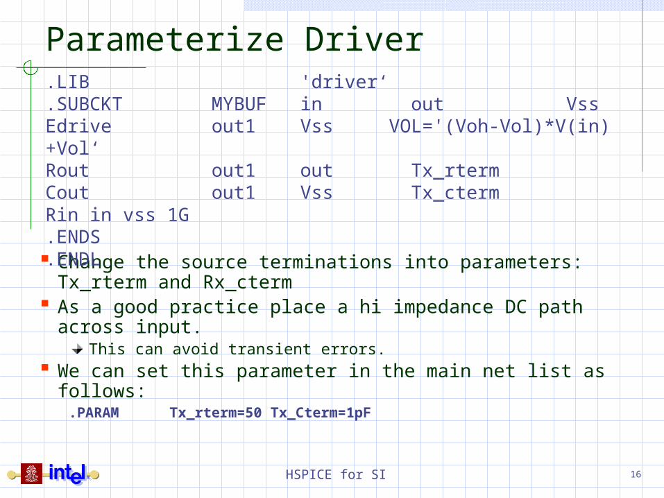
Parameterize Driver

Change the source terminations into parameters: Tx_rterm and Rx_cterm

As a good practice place a hi impedance DC path across input.

This can avoid transient errors. We can set this parameter in the main net list as

follows: .PARAM Tx_rterm=50 Tx_Cterm=1pF

.LIB 'driver‘

.SUBCKT MYBUF in out VssEdrive out1 Vss VOL='(Voh-Vol)*V(in)+Vol‘Rout out1 out Tx_rtermCout out1 Vss Tx_ctermRin in vss 1G.ENDS.ENDL

HSPICE for SI 17

Package Sub-circuit

This is a simple package that uses a coupled inductor circuit.

Often this subcircuit is more complex and derive from tools like Ansoft

.LIB 'LC_pack'

.SUBCKT PKG in1 in2 out1 out2 VssL1 in1 out1 1nL2 in2 out2 1nK1 L1 L2 0.2.ENDS.ENDL

HSPICE for SI 18

out2

out1

in2

in1

L2

L1

Coupled Inductors

KL12

L1 L2

Where L12 is the mutual inductance between inductor L1 and L2

HSPICE for SI 19

Printed wiring board modeling

Board etches can be accurately modeled with W-elements. For that case we use coupled transmission lines for the

board traces The file ‘s5_z068.9_z0d108.8.rlc’ contains the transmission

line characteristics. This data may be created with internal HSPICE 2-D field solver or any other 2-D field solver such as Ansoft.

The symbol “+” is a continuation line. Often this subcircuit can become quite substantial

containing many transmission lines and board features modeled as passive elements.

.LIB 'easy_lines‘

.SUBCKT BRD in1 in2 out1 out2 VssWline1 in1 in2 Vss out1 out2 Vss+ RLGCFILE= ‘s5_z068.9_z0d108.8' N=2L=0.1.ENDS.ENDL

HSPICE for SI 20

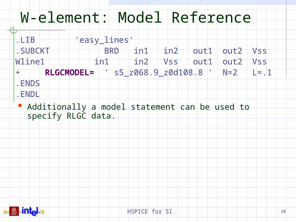
W-element: Model Reference

Additionally a model statement can be used to specify RLGC data.

.LIB 'easy_lines‘

.SUBCKT BRD in1 in2 out1 out2 VssWline1 in1 in2 Vss out1 out2 Vss+ RLGCMODEL= ' s5_z068.9_z0d108.8 ' N=2L=.1.ENDS.ENDL

HSPICE for SI 21

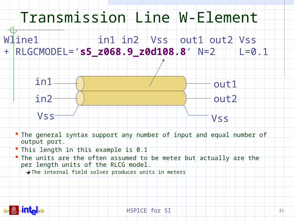
Transmission Line W-Element

The general syntax support any number of input and equal number of output port.

This length in this example is 0.1 The units are the often assumed to be meter but actually are the per length

units of the RLCG model. The internal field solver produces units in meters

Wline1 in1 in2 Vss out1 out2 Vss+ RLGCMODEL=‘s5_z068.9_z0d108.8‘ N=2 L=0.1

in1

in2

Vss Vss

out2

out1

HSPICE for SI 22

Creating a field solution

Create a file that invokes the target transmission lines.

In this file also specify:Field solver optionsMaterialsStackup

The dielectric and power/ground conductor plane sandwich of a PWB

Trace geometries shapesThe a models that include the above

HSPICE for SI 23

Couple Strip Line Example (twolines.sp)

w

ef

h

bt

tg

tg

r, tan

.Title Field SolverW2+ 1 2 0 a b 0+ Fsmodel=s5_z068.9_z0d108.8 N=2 L=1 DELAYOPT=1* s w ef t Tg * mils 5 5 0.5 0.5 1* mils converted to meters 1.270E-04 1.27E-04 1.27E-05 1.27E-05 2.54E-03* b h er tand u conduct.

* mils 0.5 10 3.90 .02 1 4.2E+07

* mils converted to meter 5.207E-04 2.54E-04

s

HSPICE for SI 24

Using the Solver

.Title Field SolverW2+ 1 2 0 a b 0+ Fsmodel=s5_z068.9_z0d108.8 N=2 L=1 DELAYOPT=1* s w ef t Tg * mils 5 5 0.5 0.5 1* mils converted to meters 1.270E-04 1.27E-04 1.27E-05 1.27E-05 2.54E-03* b h er tand u conduct.

* mils 0.5 10 3.90 .02 1 4.2E+07

* mils converted to meter 5.207E-04 2.54E-04

(cont’d on next page)

First line should be comment or title else it gets ignored

Invoking the W element will cause the field solver to run, if the

FSMODEL parameter is specified

Often this is done outside the main net list to insure solution quality. Then a

RLGCMODEL or RLGCFILE statement would be used here instead

HSPICE for SI 25

Field Solver Option Statement

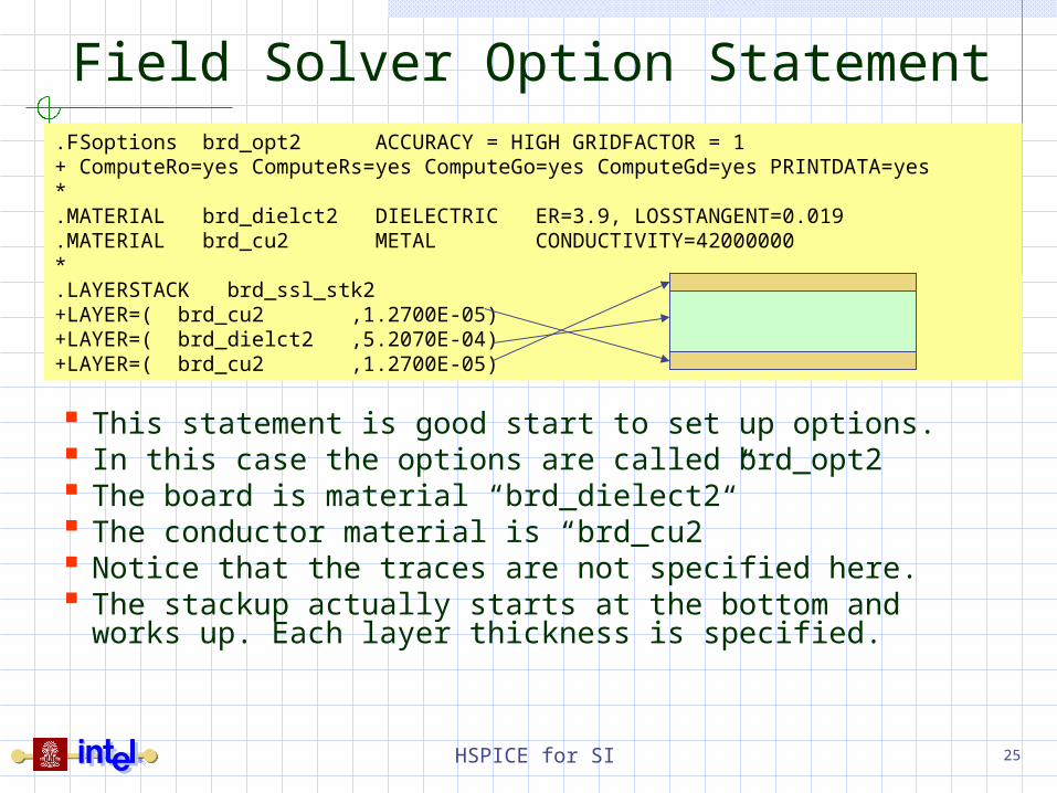
This statement is good start to set up options. In this case the options are called brd_opt2 The board is material “brd_dielect2” The conductor material is “brd_cu2” Notice that the traces are not specified here. The stackup actually starts at the bottom and

works up. Each layer thickness is specified.

.FSoptions brd_opt2 ACCURACY = HIGH GRIDFACTOR = 1+ ComputeRo=yes ComputeRs=yes ComputeGo=yes ComputeGd=yes PRINTDATA=yes*.MATERIAL brd_dielct2 DIELECTRIC ER=3.9, LOSSTANGENT=0.019.MATERIAL brd_cu2 METAL CONDUCTIVITY=42000000*.LAYERSTACK brd_ssl_stk2+LAYER=( brd_cu2 ,1.2700E-05)+LAYER=( brd_dielct2 ,5.2070E-04)+LAYER=( brd_cu2 ,1.2700E-05)

HSPICE for SI 26

Material and Shapes

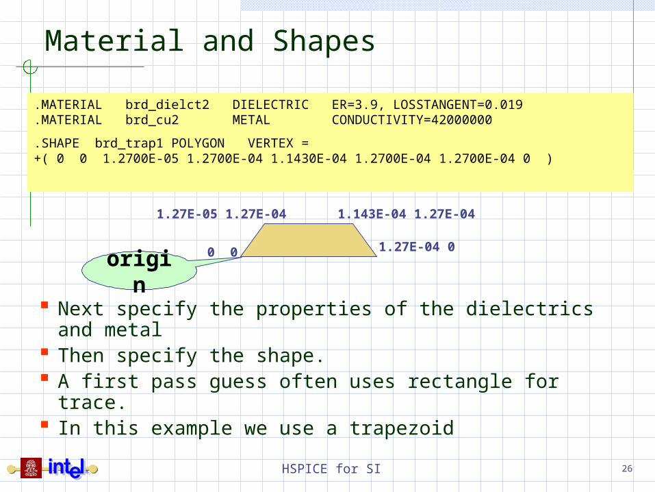
Next specify the properties of the dielectrics and metal

Then specify the shape. A first pass guess often uses rectangle for trace. In this example we use a trapezoid

0 0

1.27E-05 1.27E-04 1.143E-04 1.27E-04

1.27E-04 0

.MATERIAL brd_dielct2 DIELECTRIC ER=3.9, LOSSTANGENT=0.019

.MATERIAL brd_cu2 METAL CONDUCTIVITY=42000000

.SHAPE brd_trap1 POLYGON VERTEX =+( 0 0 1.2700E-05 1.2700E-04 1.1430E-04 1.2700E-04 1.2700E-04 0 )

origin

HSPICE for SI 27

The Model statement

Here the field solver calls out what was specified.

brd_ssl_stk2brd_opt2brd_cu2brd_trap2

.MODEL s5_z068.9_z0d108.8+W MODELTYPE=FieldSolver, LAYERSTACK=brd_ssl_stk2 FSoptions=brd_opt2+CONDUCTOR=(SHAPE=brd_trap2 MATERIAL=brd_cu2 + ORIGIN=( 6.3500E-05, 2.6670E-04)+CONDUCTOR=(SHAPE=brd_trap2 MATERIAL=brd_cu2 + ORIGIN=( -1.9050E-04, 2.6670E-04)+RLGCfile=s5_z068.9_z0d108.8.rlc.END

HSPICE for SI 28

Placing the Shapes

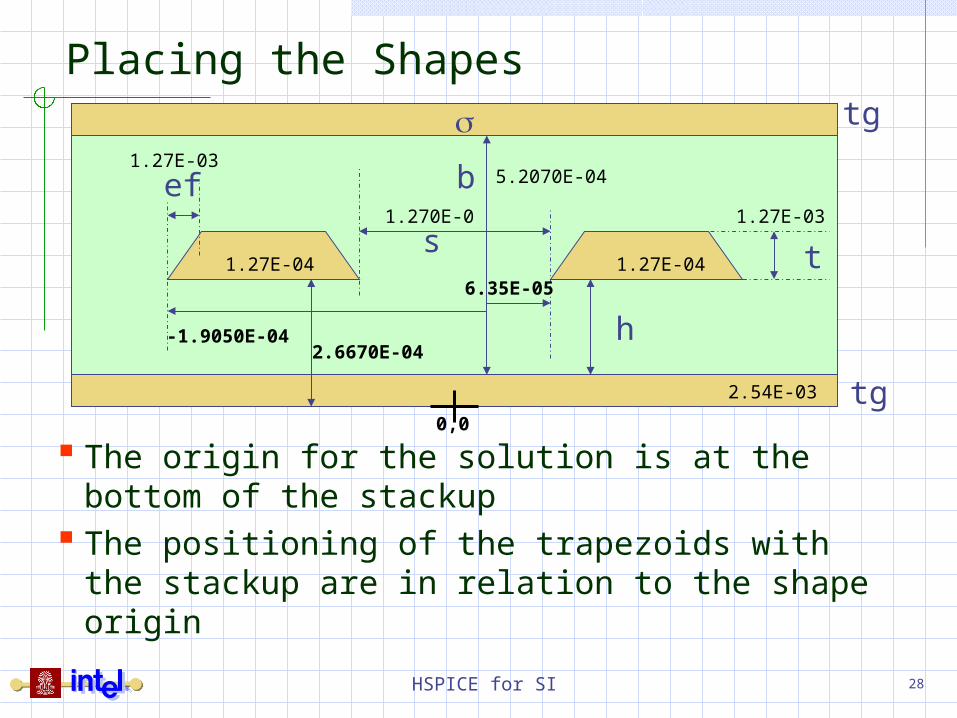
The origin for the solution is at the bottom of the stackup

The positioning of the trapezoids with the stackup are in relation to the shape origin

1.27E-04

ef

h

b

t

tg

tg1.27E-03

1.27E-03

5.2070E-04

2.54E-03

2.6670E-04

0,0

-1.9050E-04

1.27E-046.35E-05

1.270E-0

s

HSPICE for SI 29

The RLCG Model

Only half of the diagonal and the lower half of the matrix is specified

Default units are H/m, F/m, /m, S/m, /(m*srqt(Hz), S/(m*Hz) respectively

Alternatively H/in, F/in, /in, S/in, /(in*srqt(Hz), S/(in*Hz) can be used if L units are to be specified in inches.

A more detailed description can be found in the HSPICE transmission line chapter

.MODEL s5_z068.9_z0d108.8 W MODELTYPE=RLGC, N=2+ Lo = 4.460644e-007+ 9.544025e-008 4.460644e-007+ Co = 1.019475e-010+ -2.181277e-011 1.019475e-010+ Ro = 1.637366e+001+ 0.000000e+000 1.637366e+001+ Go = 0.000000e+000+ 0.000000e+000 0.000000e+000+ Rs = 2.056598e-003+ 9.268906e-005 2.056651e-003+ Gd = 1.217055e-011+ -2.604020e-012 1.217055e-011.ENDS

1.019475 1010

2.181277 1011

2.181277 1011

1.019475 1010

HSPICE for SI 30

Tline issues for SI engineers

Validation of transmission line models

Comparison to equations.Most equation are only accurate to a few ohms and have are limited to only certain ratios of trace geometry

Differential impedance equations are not readily available.

Tools to compare to measurementVector Network AnalyzerTime Domain Refectometry

HSPICE for SI 31

Receiver

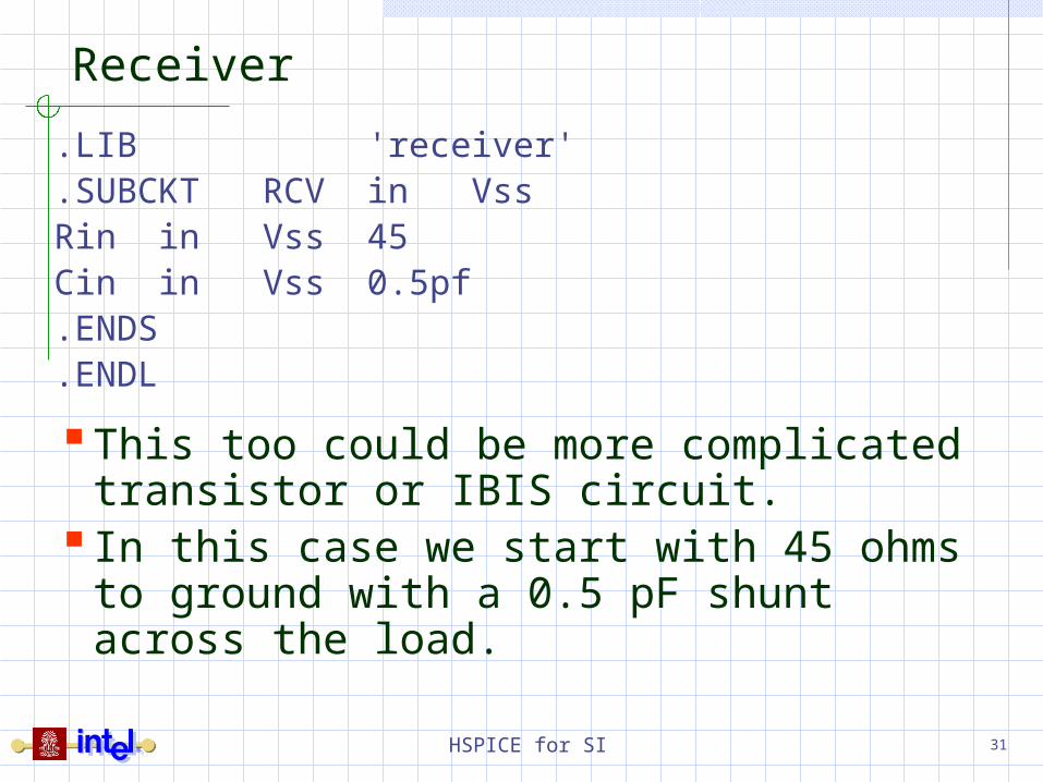
This too could be more complicated transistor or IBIS circuit.

In this case we start with 45 ohms to ground with a 0.5 pF shunt across the load.

.LIB 'receiver'

.SUBCKT RCV in VssRin in Vss 45Cin in Vss 0.5pf.ENDS.ENDL

HSPICE for SI 32

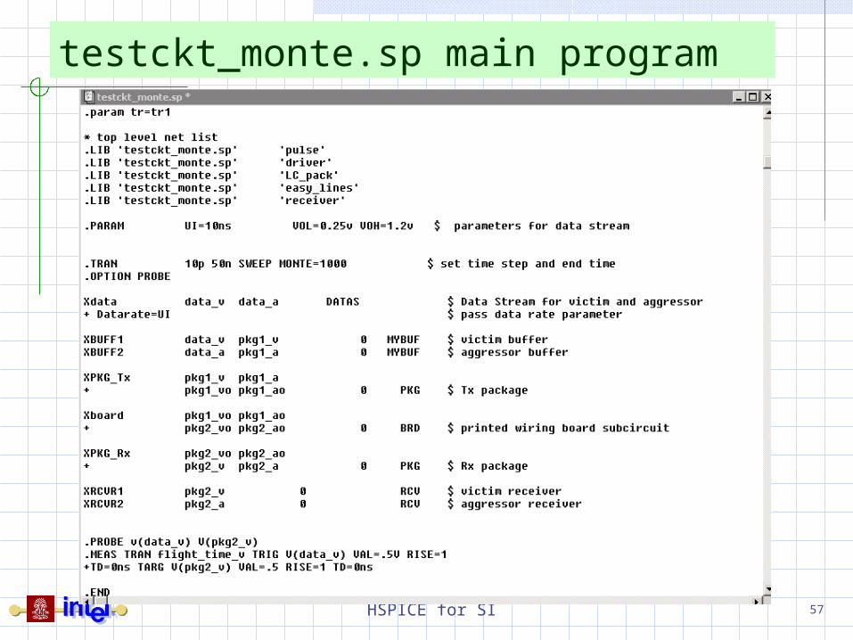
The main net list – Top Half

The libraries will go at the end for this exampleIn fact all of the above statements are position independent although parameter usage is position sensitive. Be careful if parameter are set in libraries. This can effect the order of parameter processing.

The libraries are normally in the another file. This example is not standard practice but it is convenient for collaborating on issues.

The global parameter for the bit interval UI is set to 10 nanoseconds.

Two more global parameters are used for buffer voltage control, Vol and Voh.

The transient statement tells Hspice to start a transient analysis when the “.end” statement is processed. In this case the time step interval is 10ps and will stop at 20 ns.

HSPICE for SI 33

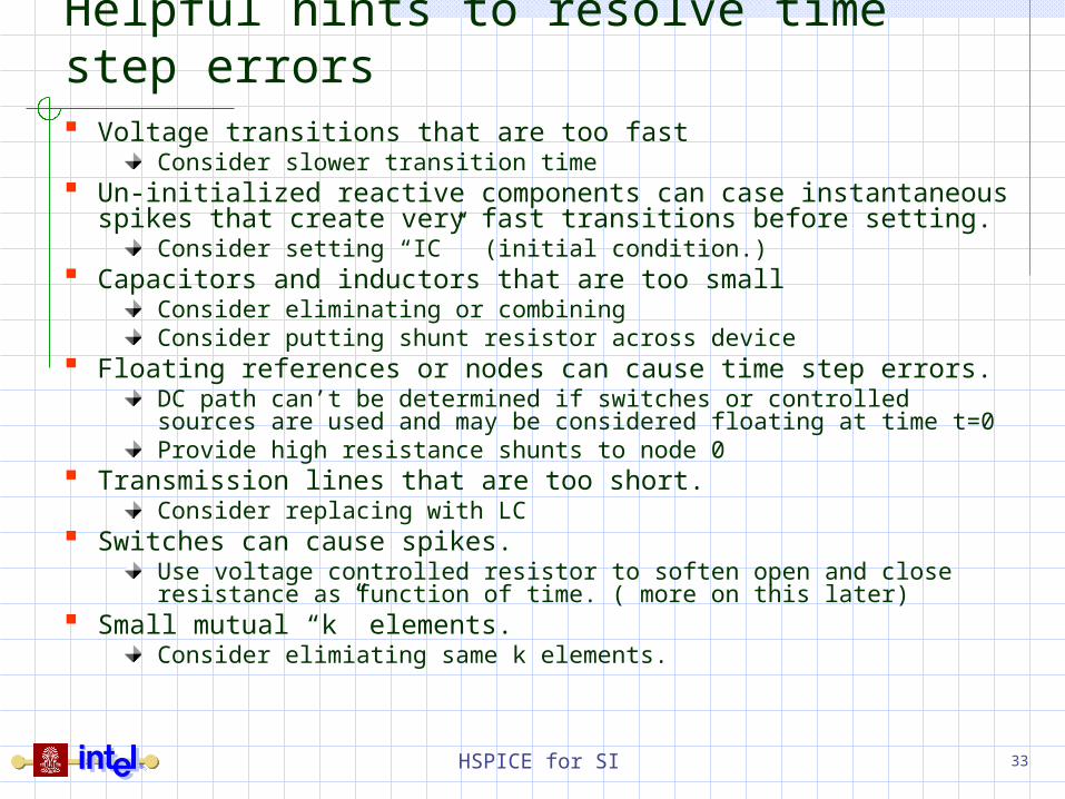
Helpful hints to resolve time step errors Voltage transitions that are too fast

Consider slower transition time Un-initialized reactive components can case instantaneous spikes

that create very fast transitions before setting.Consider setting “IC” (initial condition.)

Capacitors and inductors that are too smallConsider eliminating or combiningConsider putting shunt resistor across device

Floating references or nodes can cause time step errors.DC path can’t be determined if switches or controlled sources are used and may be considered floating at time t=0Provide high resistance shunts to node 0

Transmission lines that are too short.Consider replacing with LC

Switches can cause spikes.Use voltage controlled resistor to soften open and close resistance as function of time. ( more on this later)

Small mutual “k” elements. Consider elimiating same k elements.

HSPICE for SI 34

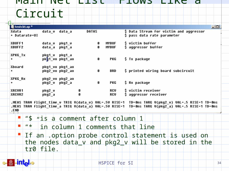
Main Net List Flows Like a Circuit

“$” is a comment after column 1 “*” in column 1 comments that line If an .option probe control statement is used on the nodes

data_v and pkg2_v will be stored in the tr0 file.

HSPICE for SI 35

Assignment Take the previous HSPICE example and draw a

circuit schematic. Produce the last picture in AvanWaves (if available) Look up and read all chapters in the HSPICE manual

on:SubcircuitsLibrariesE sourceCoupled inductorW-elementsNotice this part to the assignment is looser that most academic reading assignments. In business data-mining is a required skill. Also look up any element we cover that you do not understand.

HSPICE for SI 36

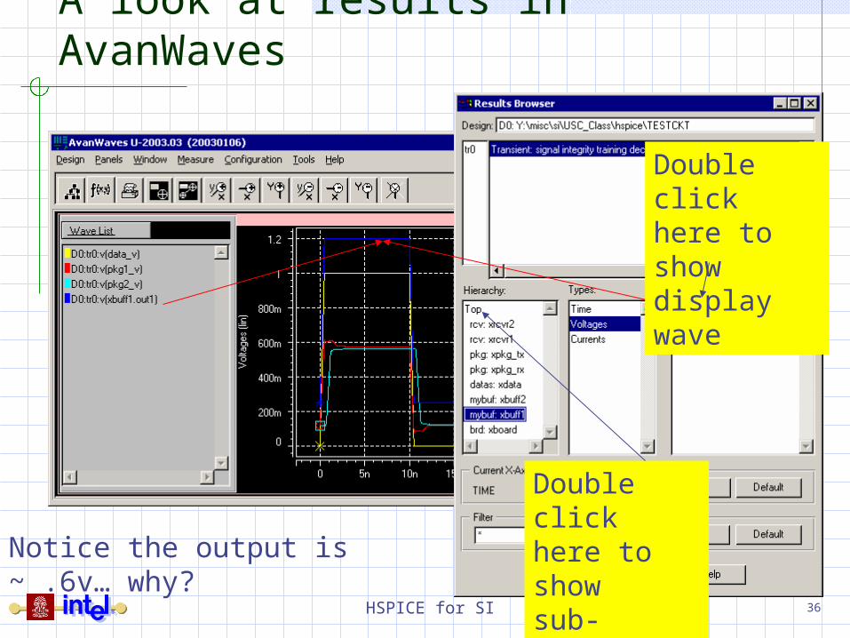
A look at results in AvanWaves

Notice the output is ~ .6v… why?

Double click here to show sub-circuit hierarchy.

Double click here to show display wave

HSPICE for SI 37

Measurement

There is a manual contain an extensive list of measurements that can be made.

In this case we are making a measurement called “flight_time_v” and “flight_time_a”

The trigger for the beginning of the measurement is at 0.5 V on the first rising on node data_v (and data_a.)

The completion of the measurement is when the first rising edge on node pkg2_v (and pkg2_a) reaches 0.5 V.

TD parameter means time delay before the measurement starts and is 0s in this example.

HSPICE for SI 38

MT0 file

This resultant MT0 file The second line is the title The third line and all the lines that follow up to the

“alter#” parameters are the parameters names. The following lines are the corresponding

measurement valuesFor this case the measurement for the parameters “flight_time_v” and “flight_time_a” are the 955.9 ps.

HSPICE for SI 39

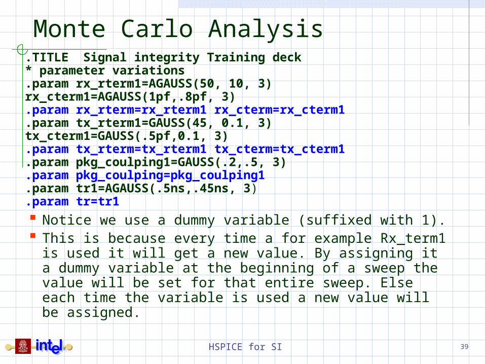
Monte Carlo Analysis

Notice we use a dummy variable (suffixed with 1). This is because every time a for example Rx_term1 is

used it will get a new value. By assigning it a dummy variable at the beginning of a sweep the value will be set for that entire sweep. Else each time the variable is used a new value will be assigned.

.TITLE Signal integrity Training deck* parameter variations.param rx_rterm1=AGAUSS(50, 10, 3) rx_cterm1=AGAUSS(1pf,.8pf, 3).param rx_rterm=rx_rterm1 rx_cterm=rx_cterm1.param tx_rterm1=GAUSS(45, 0.1, 3) tx_cterm1=GAUSS(.5pf,0.1, 3).param tx_rterm=tx_rterm1 tx_cterm=tx_cterm1.param pkg_coulping1=GAUSS(.2,.5, 3).param pkg_coulping=pkg_coulping1.param tr1=AGAUSS(.5ns,.45ns, 3).param tr=tr1

HSPICE for SI 40

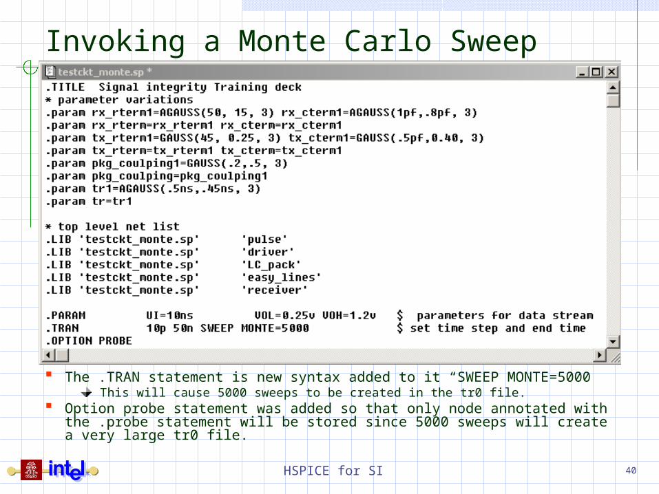
Invoking a Monte Carlo Sweep

The .TRAN statement is new syntax added to it “SWEEP MONTE=5000”This will cause 5000 sweeps to be created in the tr0 file.

Option probe statement was added so that only node annotated with the .probe statement will be stored since 5000 sweeps will create a very large tr0 file.

HSPICE for SI 41

A few changes added to the end

The “.PROBE” statement is used in conjunction with the .OPTION PROBE statement so only node data_v and pkg2_v are reported.

Only one measurement is used and the threshold was lowered to 250 mv

HSPICE for SI 42

The “Sweep” MTO file

Note each sweep entry contains the values that were assigned to the Monte Carlo parameters

A VBA or perl script is normally used (and required) to convert into a spreadsheet format

HSPICE for SI 43

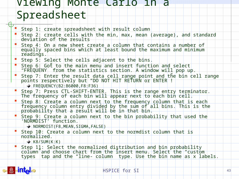
Viewing Monte Carlo in a Spreadsheet Step 1: create spreadsheet with result column Step 2: create cells with the min, max, mean (average), and standard

deviation of the results Step 4: On a new sheet create a column that contains a number of equally

spaced bins which at least bound the maximum and minimum readings. Step 5: Select the cells adjacent to the bins. Step 6: Got to the main menu and insert function and select “FREQUENY”

from the statistics section. A window will pop up. Step 7: Enter the result data cell range point and the bin cell range points

respectively but “DO NOT HIT RETURN or ENTER”!FREQUENCY(B2:B6000,F8:F36)

Step 7: Press CTL-SHIFT-ENTER. This is the range entry terminator. The frequency of each bin will appear next to each bin cell.

Step 8: Create a column next to the frequency column that is each frequency column entry divided by the sum of all bins. This is the probability that a result will be in that bin.

Step 9: Create a column next to the bin probability that used the ‘NORMDIST’ function.

NORMDIST(F8,MEAN,SIGMA,FALSE) Step 10: Create a column next to the normdist column that is normalized.

K8/SUM(K:K) Step 11: Select the normalized distribution and bin probability column and

choose chart from the insert menu. Select the “custom types” tap and the “line- column” type. Use the bin name as x labels.

HSPICE for SI 44

Check Scatter Plot First

The above scatter plot suggests that the measurements are reasonable well distributed.

Threshold = 0.35 V

Measurement Scatter

0

500

1000

0 100 200 300 400 500 600

sweep number

ps

HSPICE for SI 45

Results of Monte Carlo AnalysisBreak For spreadsheet walk throughResults below

Measured Data Top 835.9724.9 bottom 678.7784.5 bins 20743.9 SIGMA 21.71739.6 MEAN 741.31546720.6 copy of Measured Normalized Gaussian Curve

773 Bin Number Bin Values Frequencybin values PDF Gaussian for bin value708.6 1 678.70 1 678.70 0.000205 0.002 0.00028687742.3 2 686.56 4 686.56 0.000821 0.006 0.00076344755.7 3 694.42 22 694.42 0.004516 0.014 0.001782097

PDF of Measured vs. Normal

0

0.020.04

0.060.08

0.10.12

0.140.16

0.18

678.7

0

686.5

6

694.4

2

702.2

8

710.1

4

718.0

0

725.8

6

733.7

2

741.5

8

749.4

4

757.3

0

765.1

6

773.0

2

780.8

8

788.7

4

796.6

0

804.4

6

812.3

2

820.1

8

828.0

4

835.9

0

843.7

6

851.6

2

ps

pro

bab

ilit

y

Measured Estimated Gaussian

HSPICE for SI 46

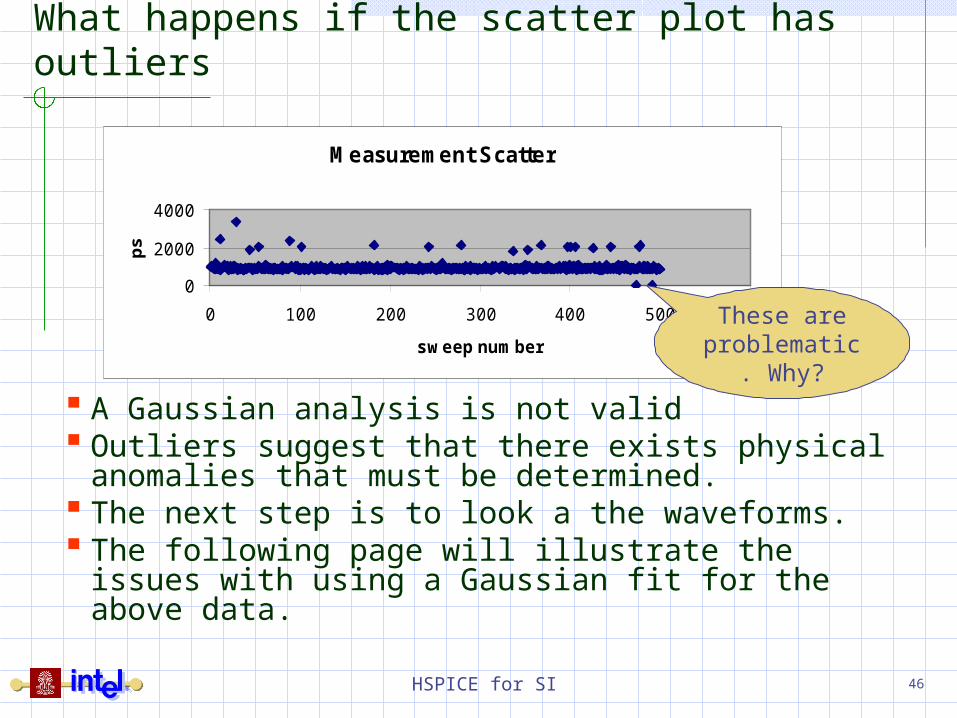
What happens if the scatter plot has outliers

A Gaussian analysis is not valid Outliers suggest that there exists physical

anomalies that must be determined. The next step is to look a the waveforms. The following page will illustrate the issues

with using a Gaussian fit for the above data.

Measurement Scatter

0

2000

4000

0 100 200 300 400 500 600

sweep number

ps

These are problematic.

Why?

HSPICE for SI 47

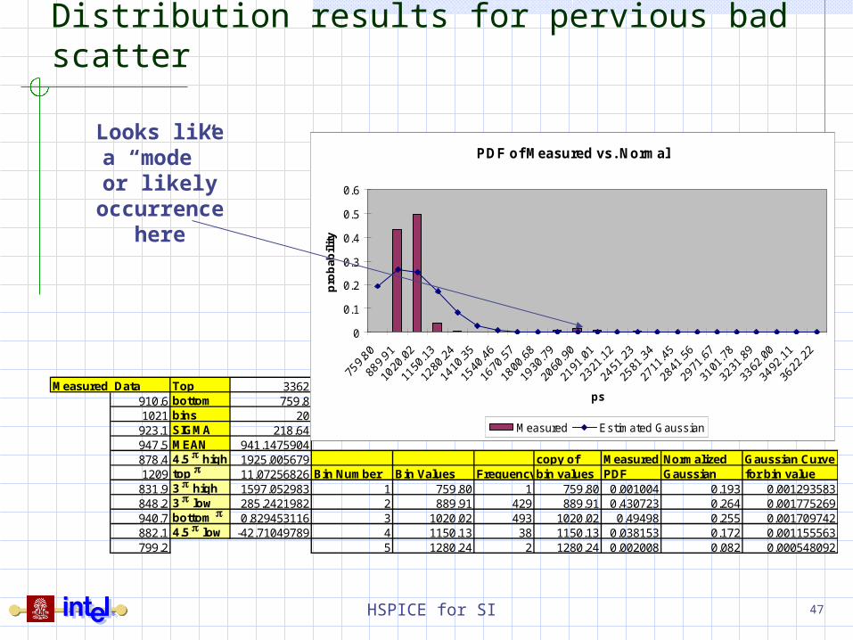
Distribution results for pervious bad scatter

Measured Data Top 3362910.6 bottom 759.81021 bins 20

923.1 SIGMA 218.64947.5 MEAN 941.1475904878.4 4.5 high 1925.005679 copy of Measured Normalized Gaussian Curve1209 top 11.07256826 Bin Number Bin Values Frequencybin values PDF Gaussian for bin value

831.9 3 high 1597.052983 1 759.80 1 759.80 0.001004 0.193 0.001293583848.2 3 low 285.2421982 2 889.91 429 889.91 0.430723 0.264 0.001775269940.7 bottom 0.829453116 3 1020.02 493 1020.02 0.49498 0.255 0.001709742882.1 4.5 low -42.71049789 4 1150.13 38 1150.13 0.038153 0.172 0.001155563799.2 5 1280.24 2 1280.24 0.002008 0.082 0.000548092

PDF of Measured vs. Normal

0

0.1

0.2

0.3

0.4

0.5

0.6

ps

pro

bab

ilit

y

Measured Estimated Gaussian

Looks like a “mode” or

likely occurrence

here

HSPICE for SI 48

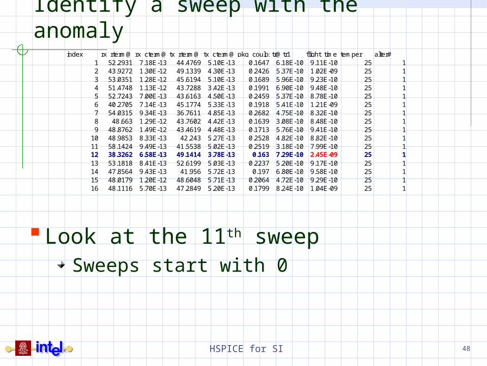
Identify a sweep with the anomaly

Look at the 11th sweepSweeps start with 0

index rx_rterm@rx_rterrx_cterm@rx_ctertx_rterm@tx_rtertx_cterm@tx_cterpkg_coulping@pkgtr@tr1 flight_time_vtemper alter#1 52.2931 7.18E-13 44.4769 5.10E-13 0.1647 6.18E-10 9.11E-10 25 12 43.9272 1.30E-12 49.1339 4.30E-13 0.2426 5.37E-10 1.02E-09 25 13 53.0351 1.28E-12 45.6194 5.10E-13 0.1689 5.96E-10 9.23E-10 25 14 51.4748 1.13E-12 43.7288 3.42E-13 0.1991 6.90E-10 9.48E-10 25 15 52.7243 7.00E-13 43.6163 4.50E-13 0.2459 5.37E-10 8.78E-10 25 16 40.2705 7.14E-13 45.1774 5.33E-13 0.1918 5.41E-10 1.21E-09 25 17 54.0315 9.34E-13 36.7611 4.85E-13 0.2682 4.75E-10 8.32E-10 25 18 48.663 1.29E-12 43.7602 4.42E-13 0.1639 3.08E-10 8.48E-10 25 19 48.8762 1.49E-12 43.4619 4.48E-13 0.1713 5.76E-10 9.41E-10 25 1

10 48.9853 8.33E-13 42.243 5.27E-13 0.2528 4.82E-10 8.82E-10 25 111 58.1424 9.49E-13 41.5538 5.02E-13 0.2519 3.18E-10 7.99E-10 25 112 38.3262 6.58E-13 49.1414 3.78E-13 0.163 7.29E-10 2.45E-09 25 113 53.1818 8.41E-13 52.6199 5.03E-13 0.2237 5.20E-10 9.17E-10 25 114 47.8564 9.43E-13 41.956 5.72E-13 0.197 6.80E-10 9.58E-10 25 115 48.0179 1.20E-12 48.6048 5.71E-13 0.2064 4.72E-10 9.29E-10 25 116 48.1116 5.70E-13 47.2849 5.20E-13 0.1799 8.24E-10 1.04E-09 25 1

HSPICE for SI 49

Break for using statistics in Excel demo

HSPICE for SI 50

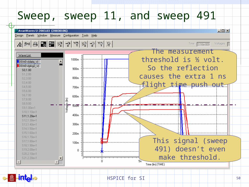
Sweep, sweep 11, and sweep 491

The measurement threshold is ½ volt. So the reflection causes the extra 1 ns flight time push out

This signal (sweep 491) doesn’t even make

threshold.

HSPICE for SI 51

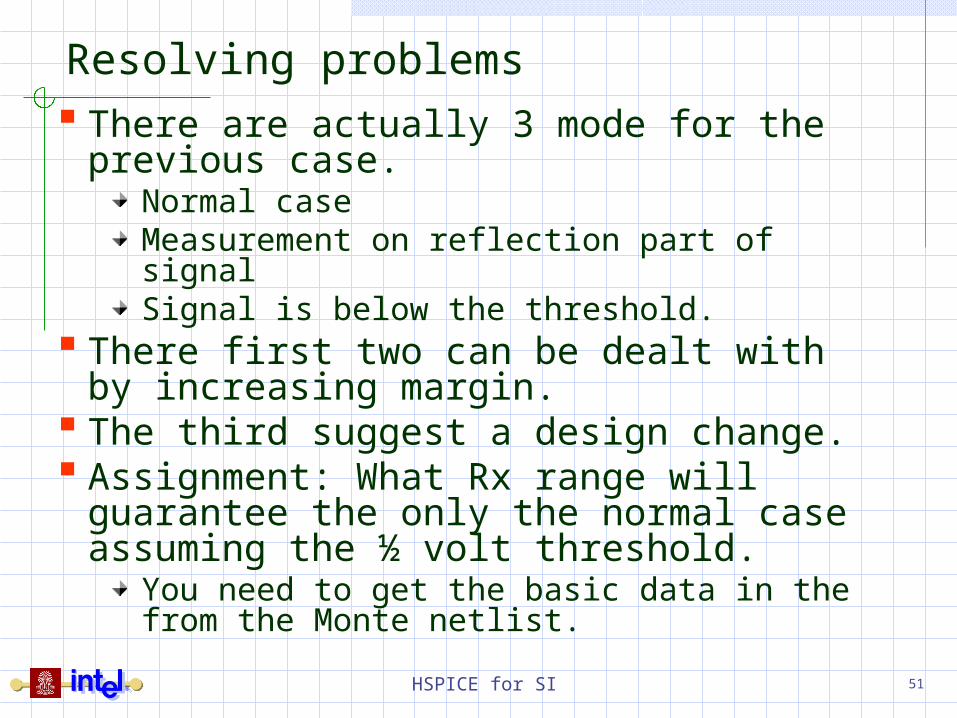
Resolving problems There are actually 3 mode for the

previous case. Normal caseMeasurement on reflection part of signalSignal is below the threshold.

There first two can be dealt with by increasing margin.

The third suggest a design change. Assignment: What Rx range will

guarantee the only the normal case assuming the ½ volt threshold.

You need to get the basic data in the from the Monte netlist.

HSPICE for SI 52

Entering Flight Time Into Budget

If the distribution looks Gaussian then most designs will use the 3 sigma numbers.

A more conservative approach would be to use 4 sigma number.

If the result are realistically bounded, but not Gaussian, the extreme limits can be used but there is a risk that the worst combination was not simulated.

HSPICE for SI 53

Backup – Hspice Listings

HSPICE for SI 54

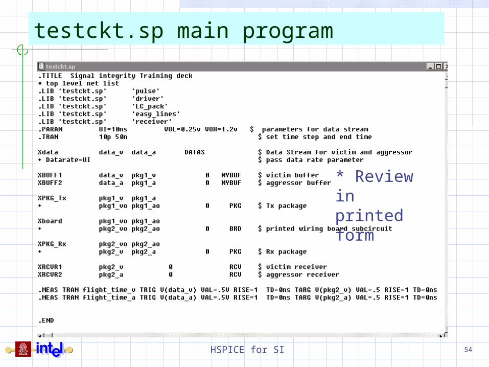
testckt.sp main program

* Review in printed form

HSPICE for SI 55

testckt.sp – libraries (cont’d)

HSPICE for SI 56

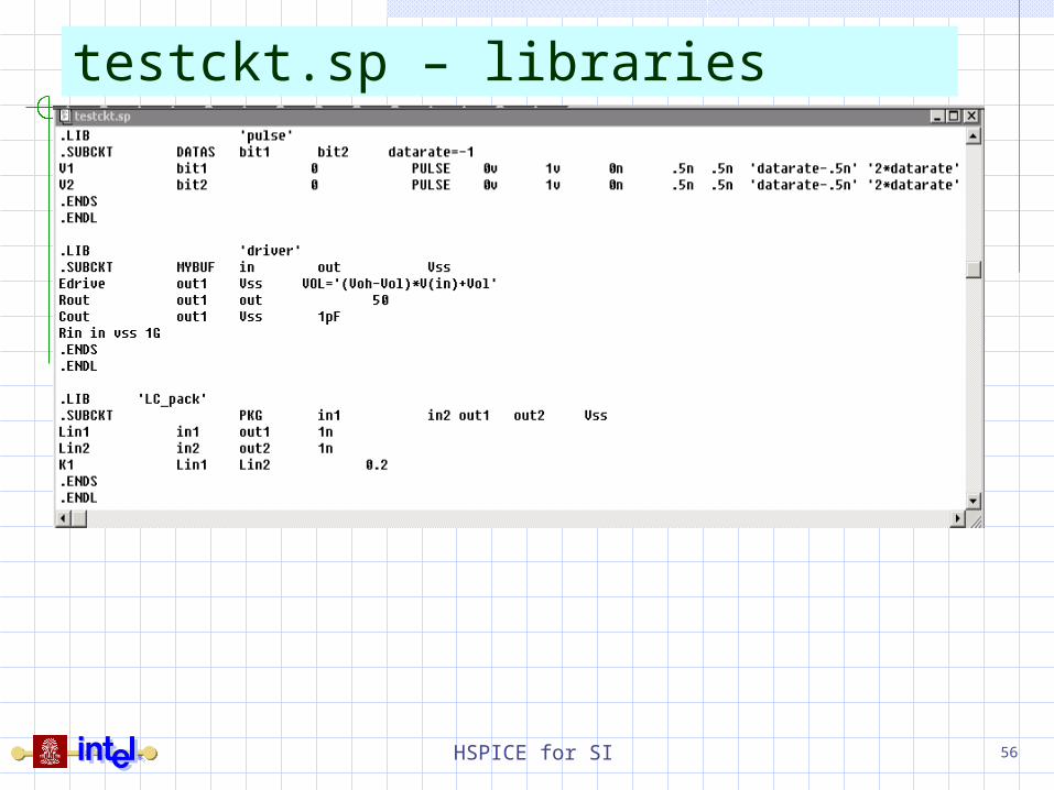
testckt.sp – libraries

HSPICE for SI 57

testckt_monte.sp main program

HSPICE for SI 58

testckt_monte.sp – libraries

HSPICE for SI 59

testckt_monte.sp – libraries (cont’d)