1 General · 1 General Fatigue failure is one of the primary damage modes of offshore ... the...
66
FATIGUE ASSESSMENT OF LIUHUA FPS (CCSI) June 2007 1 1 General Fatigue failure is one of the primary damage modes of offshore structures. The report is on the fatigue strength assessment of the Liuhua FPS, in which fatigue life of the key structural nodes of the platform are given. The fatigue analysis is completed with the fatigue strength direct computing method based on spectral analysis. According to the result of analysis, some conclusions and suggestions are given. 1.1 General Situation of the Platform Structure The LiuHua Floating Production System (FPS) is a semi-submersible mobile offshore drilling unit. It consists of two lower hulls (pontoons) which are connected by one cross pontoon at each end. From the lower hulls four corner column/sponsons and four intermediate columns rise up to support the rectangular main deck. Transverse trusses and braces are arranged between the four pairs of columns and the main deck transverse girders. 1.1.1 Principal Dimension and Other Parameters The principal dimensions and parameters of Liuhua FPS are described in Table1.1. Table 1.1 Principal characteristics of LuiHua FPS Dimensions Units/m Units/ft Length molded 90.221 296 Breadth molded 73.4568 241 Main deck Height molded 39.624 130 Length molded 89.926 295 Breadth molded 15.240 50 Lower hull height molded 6.401 21 Breadth molded 6.401 21 Cross pontoon Height molded 3.658 12 Corner column Diameter 9.144 30 Intermediate column Diameter 5.486 18 Operating draft 22.860 75 *Drafts are all from the base line.
Transcript of 1 General · 1 General Fatigue failure is one of the primary damage modes of offshore ... the...

FATIGUE ASSESSMENT OF LIUHUA FPS (CCSI) June 2007
1
1 General
Fatigue failure is one of the primary damage modes of offshore structures. The report
is on the fatigue strength assessment of the Liuhua FPS, in which fatigue life of the
key structural nodes of the platform are given. The fatigue analysis is completed with
the fatigue strength direct computing method based on spectral analysis. According to
the result of analysis, some conclusions and suggestions are given.
1.1 General Situation of the Platform Structure
The LiuHua Floating Production System (FPS) is a semi-submersible mobile offshore
drilling unit. It consists of two lower hulls (pontoons) which are connected by one
cross pontoon at each end. From the lower hulls four corner column/sponsons and
four intermediate columns rise up to support the rectangular main deck. Transverse
trusses and braces are arranged between the four pairs of columns and the main deck
transverse girders.
1.1.1 Principal Dimension and Other Parameters The principal dimensions and parameters of Liuhua FPS are described in Table1.1.
Table 1.1 Principal characteristics of LuiHua FPS
Dimensions Units/m Units/ft
Length molded 90.221 296
Breadth molded 73.4568 241 Main deck
Height molded 39.624 130
Length molded 89.926 295
Breadth molded 15.240 50 Lower hull
height molded 6.401 21
Breadth molded 6.401 21 Cross pontoon
Height molded 3.658 12
Corner column Diameter 9.144 30
Intermediate column Diameter 5.486 18
Operating draft 22.860 75
*Drafts are all from the base line.

FATIGUE ASSESSMENT OF LIUHUA FPS (CCSI) June 2007
2
Where, the lower hull is spaced 195’apart, center to center. All stability columns are
spaced 75’ apart in longitudinal direction, which have a constant diameter when
extending from the top of lower hull at 21’ level to the main deck at 130’ level.
1.1.2 General Situation of the Structure
The major structure is composed by main deck, derrick, column and sponsons,
intermediate columns, chords and lower pontoons. The basic frame is shown in
Fig.1.1.
Fig.1-1 basic frame of the calculated FPS
1.2 Data Source The basic data used in the modeling, calculations and analysis come from the
following resources:
[1] BH10101-BH10110. LOWER HULL MODIFICATIONS
[2] BH10201-BH10204. STABILITY COLUMN MODIFICATIONS-SPONSONS
[3] BH10301-BH10302. MAIN TRUSS MODIFICATIONS TUBULARS
[4]BH10401-BH10405.MAIN DECK FRAMING PLAN (ELEV. & SECTS. &
DETAIL)
FATIGUE ASSESSMENT OF LIUHUA FPS (CCSI) June 2007
3
[5] BH10501-BH10507. CONSTRUCTION PLAN COLUMN TOPS FOR CHAIN
JACKS-DETAILS
[6] BH10601-BH10602. MAIN TRUSS MODIFICATIONS JOINTS
[7] BH10701-BH10707. MAIN & INTERM GIRDER MODS -KEY PLAN & SECT.
[8] BH10801-BH10804. CHAIN FAIRLEAD SUPPORT
[9] BH10901. PORT/AFT 30'-0" COLUMN 111'-9" DECK
[10] BD00101-BD01202. GENERAL ARRANGEMENT
[11] BD01401-BD01402. CAPACITY PLAN
[12] BD01501-BD01504. ALLOWABLE DECK LOAD PLAN
[13] D01601A,B,E. INCLINING EXPERIMENT AGENDA AND PROCEDURE
[14] D01901. DOCKING PLAN
[15] D03101A,D,E,F. CONTRACTOR'S WEIGHT ESTIMATE
[16] COLUMN-D1(30FT) SITE CHECK
[17] 1971 Drawings [18] FPS Nan Hai Tiao Zhan Specialist Inspection Survey of Column
[19] FPS Nan Hai Tiao Zhan Specialist Inspection Survey of Substructure Beam
under Drilling Derrick and Main Deck
[20] Ultrasonic Wall Thickness Survey (July 2006)
[21] ABS, Rules for the Construction and Classification of Mobile Offshore Units
[22] ABS, Rules for the building and Classing Mobile Offshore drilling Units(2006)
[23] ABS, GUIDE FOR THE ASSESSMENT OF OFFSHORE STRUCTURE
FATIGUE ASSESSMENT OF LIUHUA FPS (CCSI) June 2007
4
2 Calculation Programs
The FEM was modeled by software MSC.Patran. The fatigue loads of the FPS in
regular waves calculated with 3-D linear wave load calculation program. The
powerful FEM software MSC/NASTRAN is utilized in FEM analysis.
The 3-D linear wave load calculation program was developed by the laboratory and
used in numbers of ships’ wave load calculation, and the results were much closed to
the results calculated by the software SESAM.
2.1 Theory of Wave Loads on Floating Structure
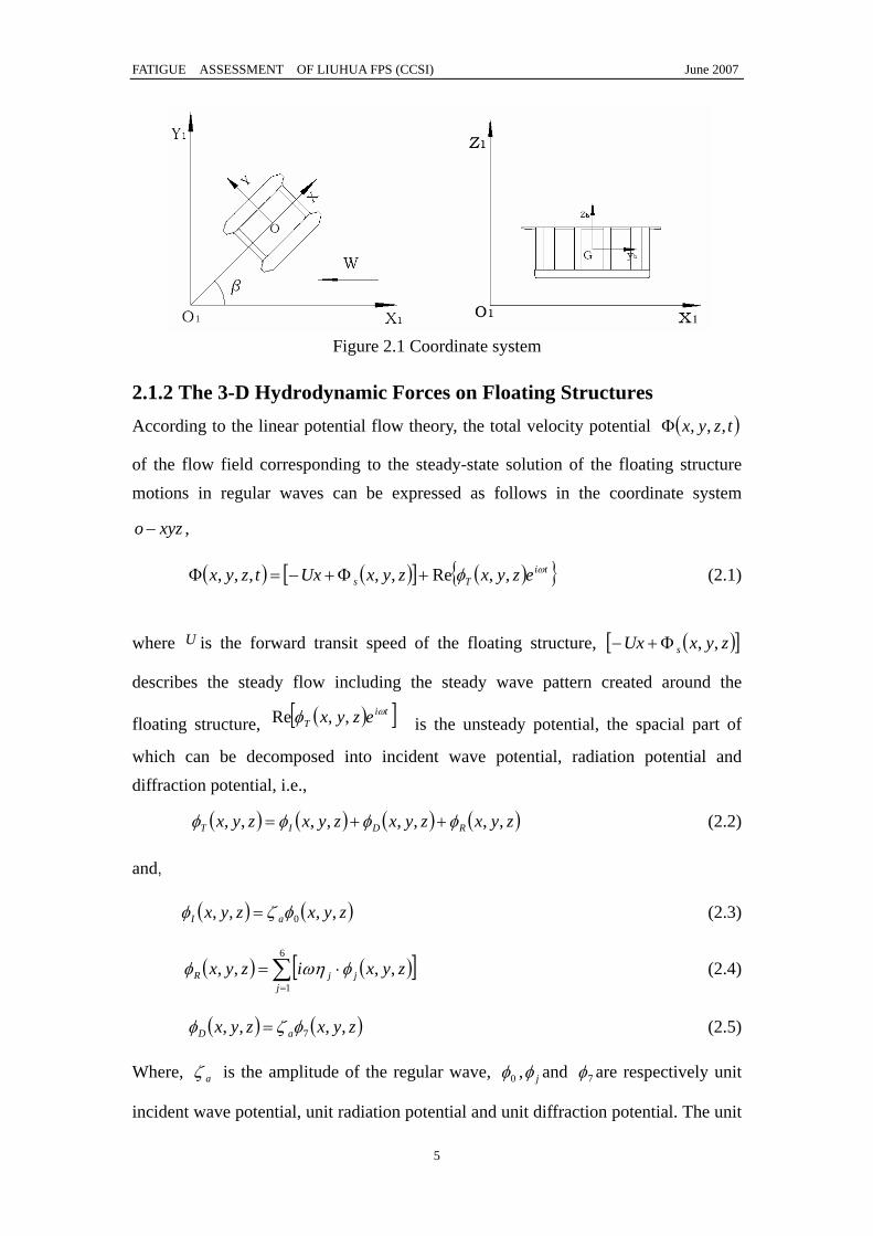
2.1.1 The Coordinate Systems
For describing incident waves,floating structure motions, velocity potential of flow as
well as sectional wave loads of the floating structure, 3 coordinate systems are built as
follows.
Coordinate system 1: (See Fig. 2.1)
The spacial fixed coordinate system 111 ZYXO − , the origin is located on the
undisturbed water surface;
Coordinate system 2: (See Fig. 2.1)
The translatory coordinate system zyxo − fixed on the mean position of the floating
structure, the xoy plane is located on the undisturbed water surface, with positive z
vertically upwards through the center of gravity of the floating structure in mean
position. On the assumption that the floating structure advances along OX -axis, and
the waves propagate at the inverse direction ofOX , the incident wave angle is β
(for head waves, o0=β ).
Coordinate system 3: (See Fig. 2.1)
The coordinate system bbb zyxG − fixed n the floating structure,the origin is G (the
center of gravity of the floating structure). The vertical coordinate of the point G is
Gz in Coordinate system 2.
FATIGUE ASSESSMENT OF LIUHUA FPS (CCSI) June 2007
5
Figure 2.1 Coordinate system
2.1.2 The 3-D Hydrodynamic Forces on Floating Structures According to the linear potential flow theory, the total velocity potential ( )tzyx ,,,Φ
of the flow field corresponding to the steady-state solution of the floating structure motions in regular waves can be expressed as follows in the coordinate system
xyzo − ,
( ) ( )[ ] ( ){ }tiTs ezyxzyxUxtzyx ωφ ,,Re,,,,, +Φ+−=Φ (2.1)
where U is the forward transit speed of the floating structure, ( )[ ]zyxUx s ,,Φ+−
describes the steady flow including the steady wave pattern created around the
floating structure, ( )[ ]tiT ezyx ωφ ,,Re is the unsteady potential, the spacial part of
which can be decomposed into incident wave potential, radiation potential and diffraction potential, i.e.,
( ) ( ) ( ) ( )zyxzyxzyxzyx RDIT ,,,,,,,, φφφφ ++= (2.2)
and,
( ) ( )zyxzyx aI ,,,, 0φζφ = (2.3)
( ) ( )[ ]∑=
⋅=6
1,,,,
jjjR zyxizyx φωηφ (2.4)
( ) ( )zyxzyx aD ,,,, 7φζφ = (2.5)
Where, aζ is the amplitude of the regular wave, 0φ , jφ and 7φ are respectively unit
incident wave potential, unit radiation potential and unit diffraction potential. The unit

FATIGUE ASSESSMENT OF LIUHUA FPS (CCSI) June 2007
6
incident wave potential is presented as follows:
[ ] )sincos(
0
0
00
0
)()(
),,( ββ
ωφ yxike
hkchhzkchigzyx −⋅
+⋅= For finite water depth (2.6)
)sincos(
00
00),,( ββ
ωφ yxikzk eeigzyx −⋅⋅= For infinite water depth (2.7)
Where, 0k is the wave number.
According to the wetted body surface condition, jφ can be decomposed into the sum
of 0jφ and u
jφ , i.e.,
ujjj i
U φω
φφ += 0 (2.8)
The unit diffraction potential 7φ and the radiation potential 0jφ , u
jφ satisfy the
boundary conditions for floating structure with a forward transit speed. It is very complicated to solve the problem of complete solution with a forward speed, and some hypotheses are applied for simplifying the calculation.
If neglecting the steady perturbation potential sΦ , we have
⎪⎩
⎪⎨
⎧
−==
==
026
035
)4~1(0
φφφφ
φ
u
u
uj j
(2.9)
On the assumption that the wave frequency is not low and the forward speed is not high, we have
xU∂∂
>>ω
(2.10)
And,
22
ωω −≈⎟⎠⎞
⎜⎝⎛
∂∂
−x
Ui (2.11)
The unit radiation potential 0jφ and unit diffraction potential 0
7φ satisfy the
following equations: for conditions in the fluid domain [L],
)7,,2,1(002 L==∇ jjφ (2.12)
For linearized free surface condition [F],

FATIGUE ASSESSMENT OF LIUHUA FPS (CCSI) June 2007
7
)7,,2,1,0(0020
L===−∂
∂jz
zg j
j φωφ
(2.13)
For body surface condition [S],
⎪⎩
⎪⎨
⎧
==∂∂
∂∂
−=∂∂
)6,,2,1(0
007
Ljnn
nn
jjφ
φφ
(2.14)
For bottom condition [B],
)7,,2,1,(00 ⋅⋅⋅=−==∂∂ jhzz jφ For definite water depth (2.15)
)7,,2,1,(0 ⋅⋅⋅=−∞→→∇ jzjφ For indefinite water depth (2.16)
For radiation condition [R]:
)7,,2,1(0)(lim 00
0
L==−∂
∂∞→
jikR
R jj
Rφ
φ (2.17)
It is shown that the above boundary conditions are completely in the same form
except that the natural circular frequency 0ω of wave is substituted by the circular
frequency of encounter ω for floating structures of zero forward speed.
The solution for 0jφ can be obtained by distributive source technique. The velocity
potential 0jφ is expressed in the form of the distributed source on the body surface, as
( ) ( ) ( )∫∫=S
qj
j dSqpGqp ,)(0 σφ (2.18)
Where, ( )qj)(σ is the strength of source, ( )qpG , is Green’s Function satisfying all
the boundary conditions but that of body surface.
According to the body surface condition of the velocity potential 0jφ , the strength of
source ( )qj )(σ satisfies the following integral equation,
( ) ( ) ( )⎪⎩
⎪⎨
⎧∂∂
−=
∂∂
+ ∫∫)(
0)()()( ,2p
j
p
Sq
p
jj
nndSqpG
nqp
φσπσ (2.19)
( p is on body surface)

FATIGUE ASSESSMENT OF LIUHUA FPS (CCSI) June 2007
8
Corresponding to the incident wave potential (for infinite or finite water depth), the
tree-dimensional Green’s Function in frequency domain for zero forward speed is
applied. The above integral equation can be transformed into linear algebra equations
by using the panel element method, and the equations can be solved. Then the
diffraction potential and radiation potential can be obtained.
Because the water depth where LiuHua_FPS operates is far beyond the wavelength,
the infinite water depth is adopted in this computation. When the platform is under
operational or survival conditions, the forward speed U is taken as zero.
2.1.3 The Equations of Floating Structure Motions
According to the dynamics of rigid body, the equations of the floating structure
motions with the center of gravity G being the center of moment can be expressed as,
[ ] { } { } { } tieFtFtM ωη ⋅==⋅ )()(&& (2.20)
where [ ]M is the generalized mass matrix of the floating structure, { })(tF is the
vector of fluid loads on the floating structure, which exclude the still water buoyant force in balance with the gravity of the floating structure.
The fluid loads acting on the floating structure can be divided into the
hydrostatic restoring loads { })(tF S induced by the displacement of the floating
structure from the mean position, the hydrodynamic loads { })(tF D depending on the
waves and floating structure motions, namely
{ } { } { })()()( tFtFtF DS += (2.21)
The hydrostatic restoring loads can be obtained by static of the floating structure,
{ } [ ]{ })()( tCtF S η−= (2.22)
Where, [ ]C is the matrix of hydrostatic restoring force coefficients.
The hydrodynamic loads can be obtained by integrating the hydrodynamic pressures on the wet surface of the floating structure. According to the division of the velocity
potential of flow,the hydrodynamic loads can be decomposed into incident wave
force, diffraction wave force and radiation force, i.e.,

FATIGUE ASSESSMENT OF LIUHUA FPS (CCSI) June 2007
9
{ } { } { } { })()()()( tFtFtFtF RDID ++= (2.23)
The incident wave force and diffraction wave force can be combined as the so-called wave excitation loads,
{ } { } { })()()( tFtFtf DI += (2.24)
The radiation force can be expressed as,
( ){ } [ ] ( ){ } [ ] ( ){ }tBtAtFR ηη &&& −−= (2.25)
Where, [ ]A and [ ]B are the matrix of three-dimensional hydrodynamic coefficients.
Eq.(2.20) representing the equations of floating structure motions in regular waves can be written as, by taken into consideration of above forces and moments,
[ ] [ ]( ) ( ){ } [ ] ( ){ } [ ] ( ){ } ( ){ } { } tieftftCtBtAM ωηηη ==++⋅+ &&& (2.26)
2.1.4 The Fluid Dynamic Pressure and Sectional Loads on The Floating Structures
Once the solution of velocity potential )7,,2,1( L=jjφ and the steady-state
solution )6,,2,1( L=jjη of the floating structure motion responses in regular
waves have been obtained, the radiation potential Rφ and the diffraction potential
Dφ can be determined by Eq.(3) and Eq.(4). By including the contribution of the
hydrostatic restoring force, the total fluid dynamic pressure can be obtained by
linearized Bernoulli’s Equation,
( ) ( )[ ]( ) ( )[
( ) ( )]⎪⎭
⎪⎬
⎫
++⋅⋅−=
=
zyxzyxzyxizyxpzyxp
ezyxptzyxP
RD
IS
ti
,,,,,,),,(,,
,,Re,,,
φφφωρ
ω
(2.27)
Where, )(),,( 543 ηηηρ xygzyxpS −+−= .
Thus, the fluid dynamic pressure on the controlling point of each panel element can
be obtained, and the fluid dynamic pressure distribution on the floating structure hull
can be given.
When the floating structure motions and the fluid dynamic pressure loads are given,
FATIGUE ASSESSMENT OF LIUHUA FPS (CCSI) June 2007
10
the wave-induced forces and moments in the sections of floating structure hull can be
calculated by using D’Alembert’s Principle, which include the vertical and horizontal
shear forces and moments as well as torsional moments.
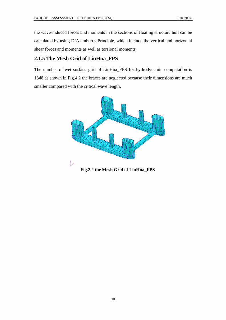
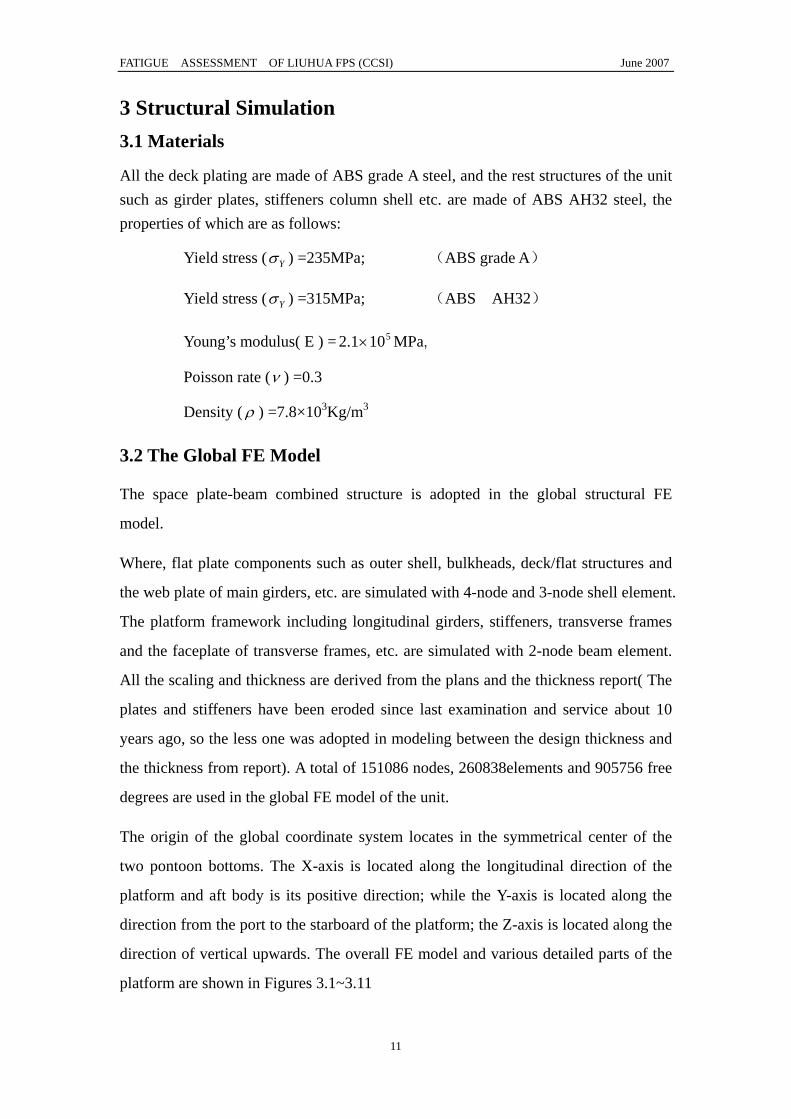
2.1.5 The Mesh Grid of LiuHua_FPS
The number of wet surface grid of LiuHua_FPS for hydrodynamic computation is
1348 as shown in Fig.4.2 the braces are neglected because their dimensions are much
smaller compared with the critical wave length.
Fig.2.2 the Mesh Grid of LiuHua_FPS
FATIGUE ASSESSMENT OF LIUHUA FPS (CCSI) June 2007
11
3 Structural Simulation 3.1 Materials
All the deck plating are made of ABS grade A steel, and the rest structures of the unit such as girder plates, stiffeners column shell etc. are made of ABS AH32 steel, the properties of which are as follows:
Yield stress ( Yσ ) =235MPa; (ABS grade A)
Yield stress ( Yσ ) =315MPa; (ABS AH32)
Young’s modulus( E ) = 5101.2 × MPa,
Poisson rate (ν ) =0.3
Density ( ρ ) =7.8×10³Kg/m3
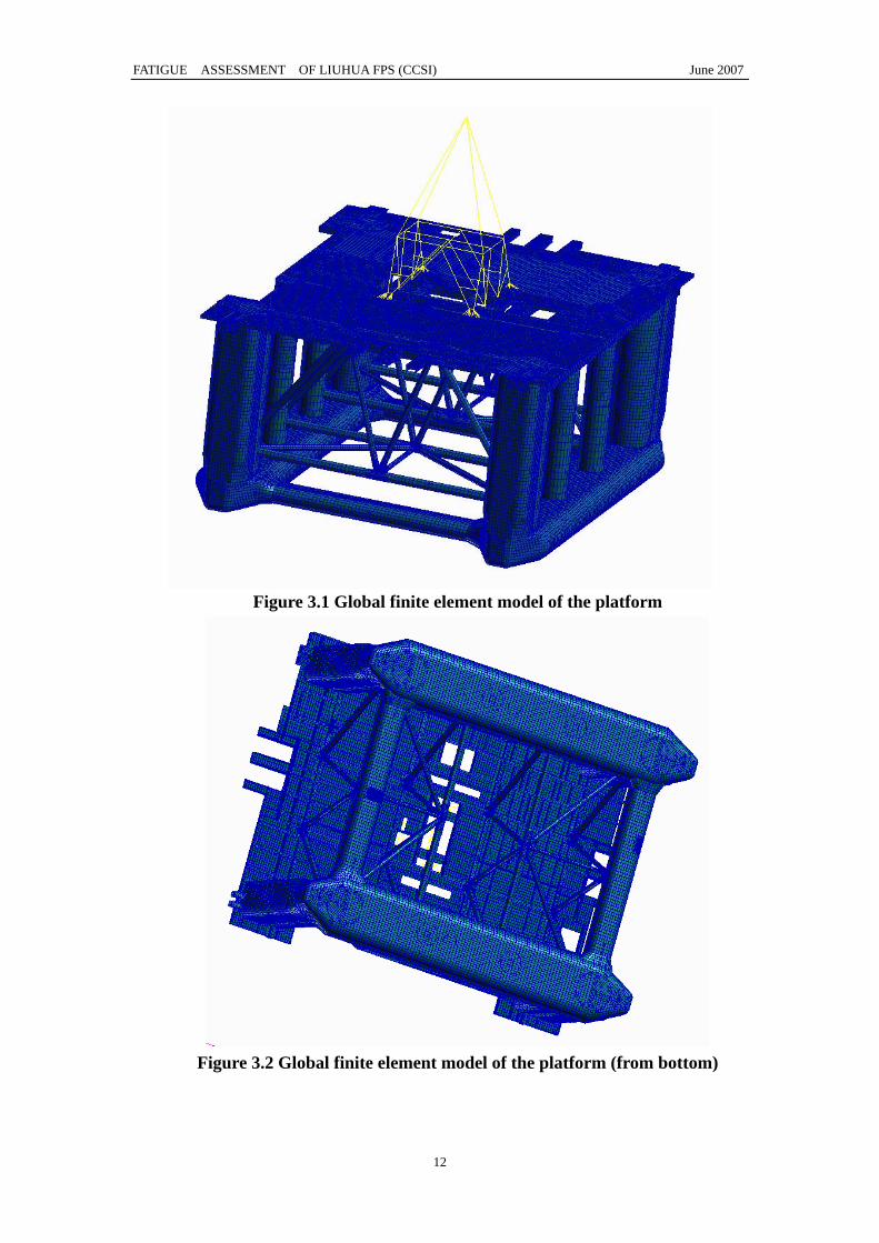
3.2 The Global FE Model
The space plate-beam combined structure is adopted in the global structural FE
model.
Where, flat plate components such as outer shell, bulkheads, deck/flat structures and
the web plate of main girders, etc. are simulated with 4-node and 3-node shell element.
The platform framework including longitudinal girders, stiffeners, transverse frames
and the faceplate of transverse frames, etc. are simulated with 2-node beam element.
All the scaling and thickness are derived from the plans and the thickness report( The
plates and stiffeners have been eroded since last examination and service about 10
years ago, so the less one was adopted in modeling between the design thickness and
the thickness from report). A total of 151086 nodes, 260838elements and 905756 free
degrees are used in the global FE model of the unit.
The origin of the global coordinate system locates in the symmetrical center of the
two pontoon bottoms. The X-axis is located along the longitudinal direction of the
platform and aft body is its positive direction; while the Y-axis is located along the
direction from the port to the starboard of the platform; the Z-axis is located along the
direction of vertical upwards. The overall FE model and various detailed parts of the
platform are shown in Figures 3.1~3.11
FATIGUE ASSESSMENT OF LIUHUA FPS (CCSI) June 2007
12
Figure 3.1 Global finite element model of the platform
Figure 3.2 Global finite element model of the platform (from bottom)

FATIGUE ASSESSMENT OF LIUHUA FPS (CCSI) June 2007
13
Figure 3.3 Global finite element model of the platform
Figure 3.4 Global finite element Model of the main deck and derrick

FATIGUE ASSESSMENT OF LIUHUA FPS (CCSI) June 2007
14
Figure 3.5 finite element model of the stability columns and sponsons
Figure 3.6 finite element model of the inner structure of the column and sponson
FATIGUE ASSESSMENT OF LIUHUA FPS (CCSI) June 2007
15
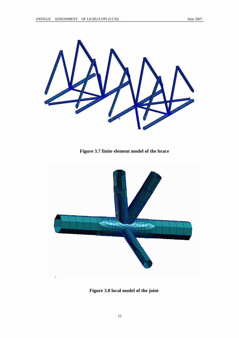
Figure 3.7 finite element model of the brace
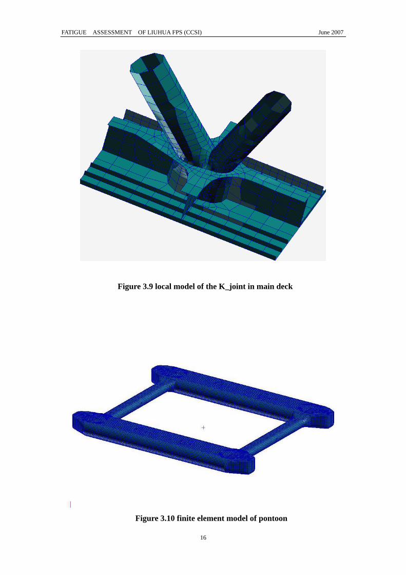
Figure 3.8 local model of the joint
FATIGUE ASSESSMENT OF LIUHUA FPS (CCSI) June 2007
16
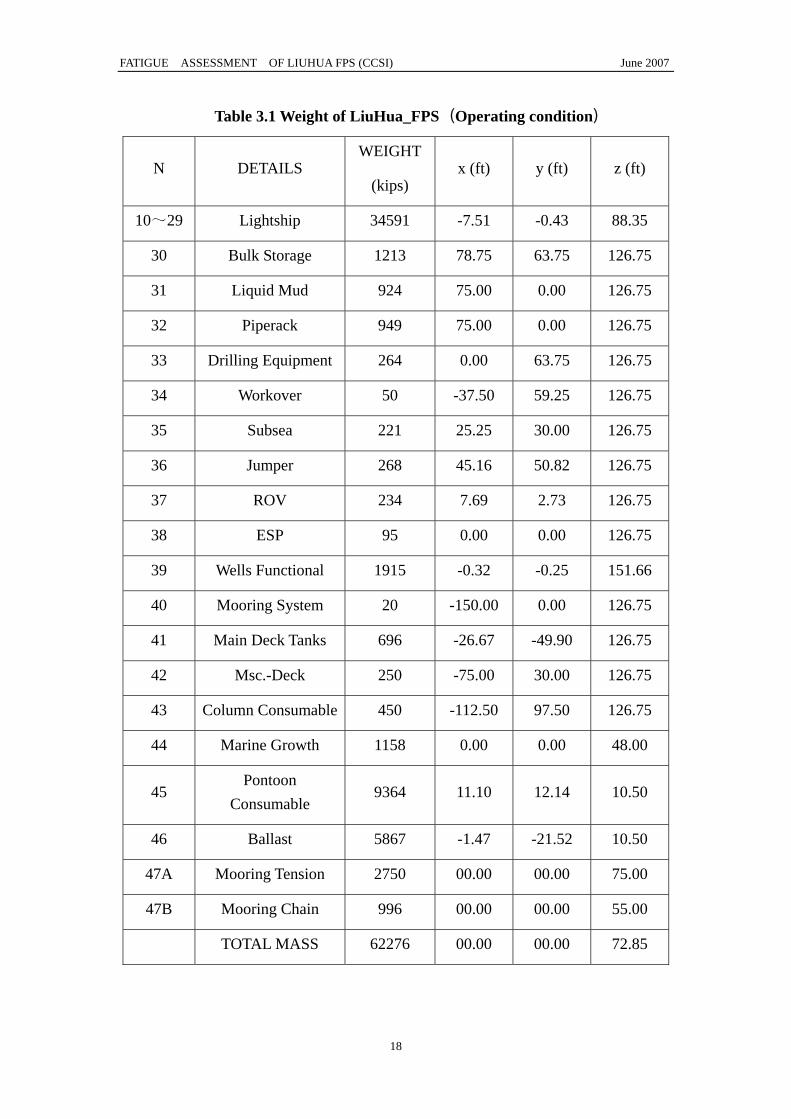
Figure 3.9 local model of the K_joint in main deck
Figure 3.10 finite element model of pontoon

FATIGUE ASSESSMENT OF LIUHUA FPS (CCSI) June 2007
17
Figure 3.11 finite element model of the inner structure of pontoon
3.3 The Adjust of Weight Distribution and Boundary Condition
In order to simulate the real statement of the structures, the weight of superstructures
and equipments needs to be taken into account. The one-node elements with mass are
adopted here.
After the balance of gravity of buoyancy was adjusted, the inertial relief method (a
function of MSC.NASTRAN) is adopted to deal with the boundary condition. In this
function, the program computes the acceleration of every node. The law of inertia is
adopted in order to form an equation. By this way the displacement of every node can
be computed.
FATIGUE ASSESSMENT OF LIUHUA FPS (CCSI) June 2007
18
Table 3.1 Weight of LiuHua_FPS(Operating condition)
N DETAILS WEIGHT
(kips) x (ft) y (ft) z (ft)
10~29 Lightship 34591 -7.51 -0.43 88.35
30 Bulk Storage 1213 78.75 63.75 126.75
31 Liquid Mud 924 75.00 0.00 126.75
32 Piperack 949 75.00 0.00 126.75
33 Drilling Equipment 264 0.00 63.75 126.75
34 Workover 50 -37.50 59.25 126.75
35 Subsea 221 25.25 30.00 126.75
36 Jumper 268 45.16 50.82 126.75
37 ROV 234 7.69 2.73 126.75
38 ESP 95 0.00 0.00 126.75
39 Wells Functional 1915 -0.32 -0.25 151.66
40 Mooring System 20 -150.00 0.00 126.75
41 Main Deck Tanks 696 -26.67 -49.90 126.75
42 Msc.-Deck 250 -75.00 30.00 126.75
43 Column Consumable 450 -112.50 97.50 126.75
44 Marine Growth 1158 0.00 0.00 48.00
45 Pontoon
Consumable 9364 11.10 12.14 10.50
46 Ballast 5867 -1.47 -21.52 10.50
47A Mooring Tension 2750 00.00 00.00 75.00
47B Mooring Chain 996 00.00 00.00 55.00
TOTAL MASS 62276 00.00 00.00 72.85
FATIGUE ASSESSMENT OF LIUHUA FPS (CCSI) June 2007
19
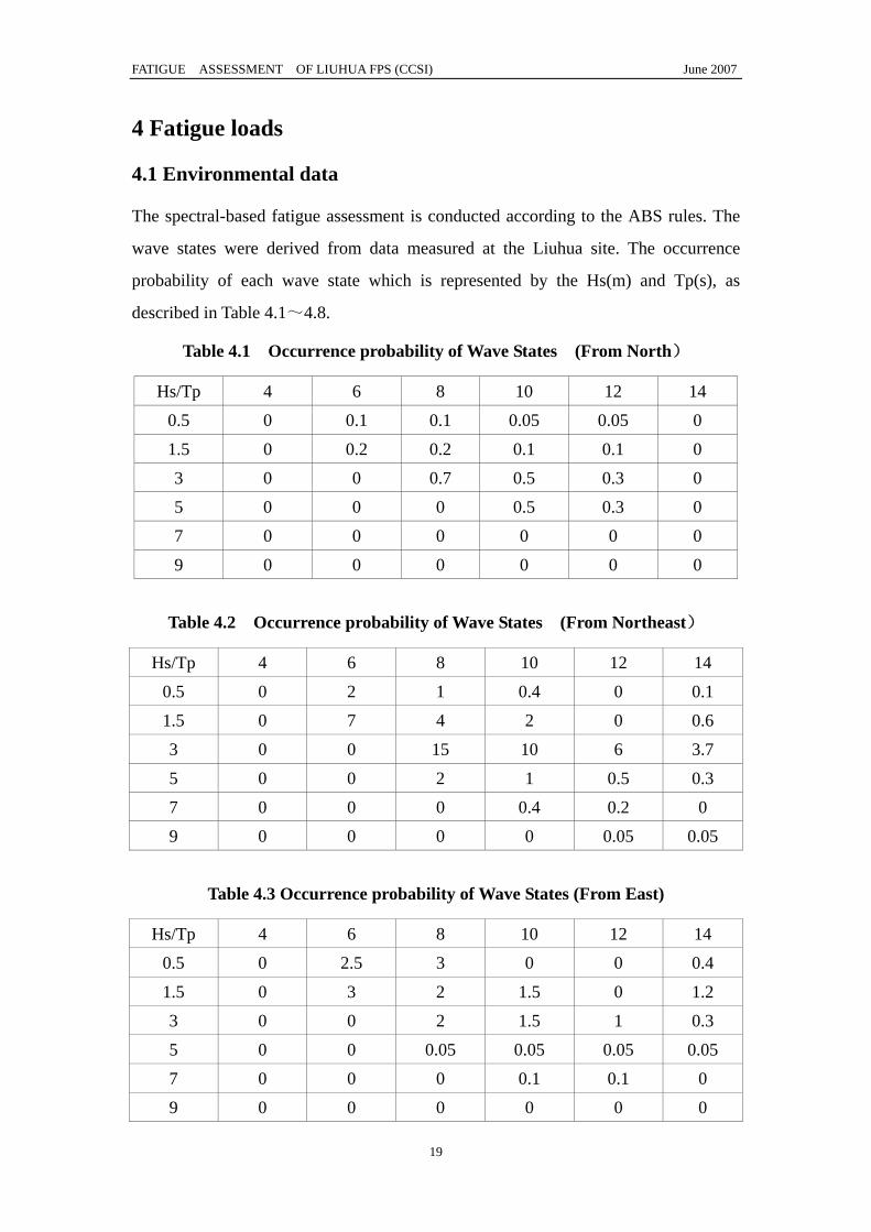
4 Fatigue loads
4.1 Environmental data
The spectral-based fatigue assessment is conducted according to the ABS rules. The
wave states were derived from data measured at the Liuhua site. The occurrence
probability of each wave state which is represented by the Hs(m) and Tp(s), as
described in Table 4.1~4.8.
Table 4.1 Occurrence probability of Wave States (From North)
Hs/Tp 4 6 8 10 12 14
0.5 0 0.1 0.1 0.05 0.05 0
1.5 0 0.2 0.2 0.1 0.1 0
3 0 0 0.7 0.5 0.3 0
5 0 0 0 0.5 0.3 0
7 0 0 0 0 0 0
9 0 0 0 0 0 0
Table 4.2 Occurrence probability of Wave States (From Northeast)
Hs/Tp 4 6 8 10 12 14
0.5 0 2 1 0.4 0 0.1
1.5 0 7 4 2 0 0.6
3 0 0 15 10 6 3.7
5 0 0 2 1 0.5 0.3
7 0 0 0 0.4 0.2 0
9 0 0 0 0 0.05 0.05
Table 4.3 Occurrence probability of Wave States (From East)
Hs/Tp 4 6 8 10 12 14
0.5 0 2.5 3 0 0 0.4
1.5 0 3 2 1.5 0 1.2
3 0 0 2 1.5 1 0.3
5 0 0 0.05 0.05 0.05 0.05
7 0 0 0 0.1 0.1 0
9 0 0 0 0 0 0
FATIGUE ASSESSMENT OF LIUHUA FPS (CCSI) June 2007
20
Table4.4 Occurrence probability of Wave States (From Southeast)
Hs/Tp 4 6 8 10 12 14
0.5 0 1 0.6 0.4 0.2 0
1.5 0 0.2 0.2 0.1 0.1 0
3 0 0.3 0.3 0.2 0.1 0
5 0 0 0 0 0 0
7 0 0 0 0 0 0
9 0 0 0 0 0 0
Table4.5 Occurrence probability of Wave States (From South)
Hs/Tp 4 6 8 10 12 14
0.5 0 1 0.5 0.5 0.4 0
1.5 0 2 1 0.4 0.2 0
3 0 0.8 0.4 0.3 0.2 0
5 0 0 0.05 0.1 0.05 0
7 0 0 0 0 0 0
9 0 0 0 0 0 0
Table4.6 Occurrence probability of Wave States (From Southwest)
Hs/Tp 4 6 8 10 12 14
0.5 0 2 0.7 0.4 0.2 0
1.5 0 2.5 1 0.6 0.4 0
3 0 0.2 0.2 0.1 0.1 0
5 0 0 0 0 0 0
7 0 0 0 0 0 0
9 0 0 0 0 0 0
Table4.7 Occurrence probability of Wave States (From West)
Hs/Tp 4 6 8 10 12 14
0.5 0.4 0.3 0.2 0.1 0 0
1.5 0.1 0.1 0.05 0.05 0 0
3 0 0 0 0 0 0
5 0 0 0 0 0 0
7 0 0 0 0 0 0
9 0 0 0 0 0 0
FATIGUE ASSESSMENT OF LIUHUA FPS (CCSI) June 2007
21
Table4.8 Occurrence probability of Wave States (From Northwest)
Hs/Tp 4 6 8 10 12 14
0.5 0.05 0.05 0.1 0 0 0
1.5 0.05 0.05 0.05 0.05 0 0
3 0 0 0 0 0 0
5 0 0 0 0 0 0
7 0 0 0 0 0 0
9 0 0 0 0 0 0
4.2 The Parameters for the Calculation of Fatigue Loads
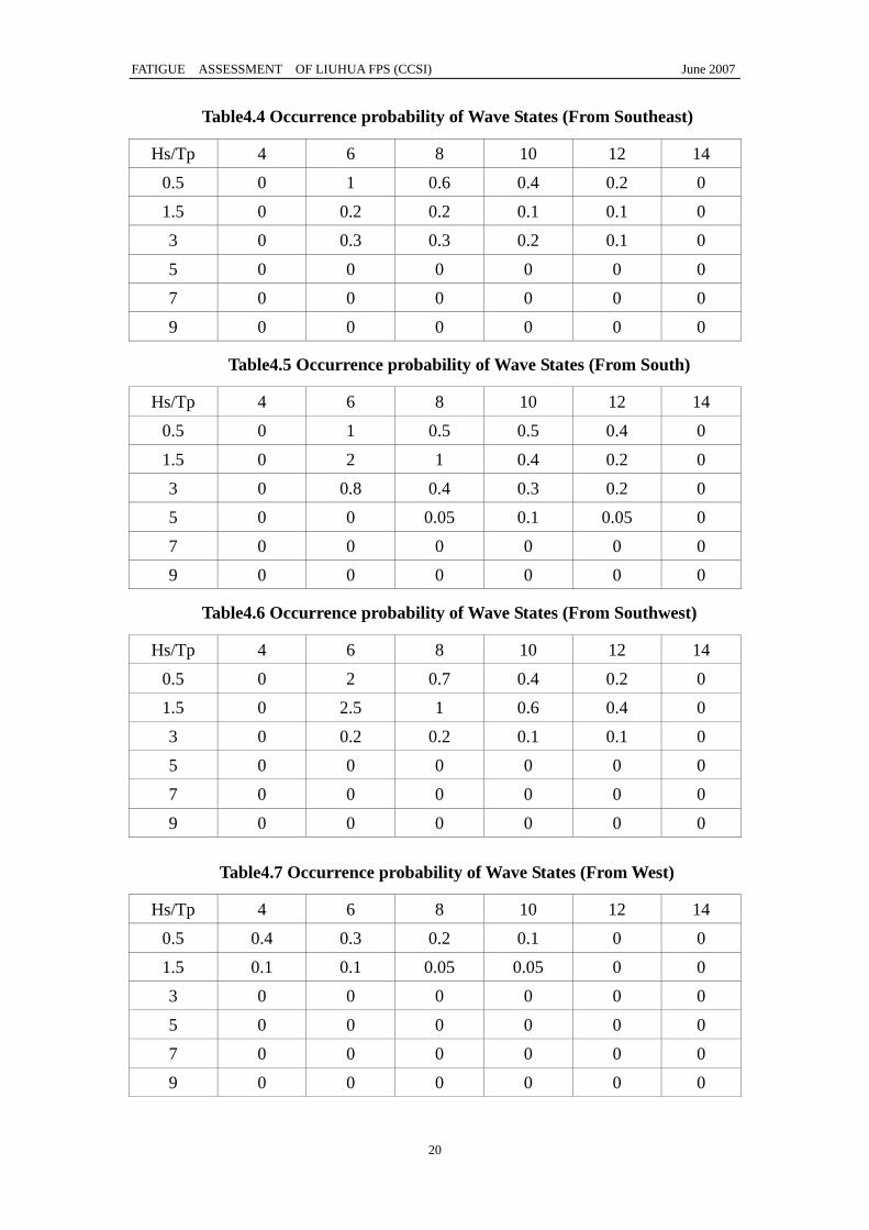
4.2.1 Wave Directions
Eight wave directions are chosen when computing the fatigue loads. Fig 3.1 shows the
position of the platform and wave directions. The occurrence of each wave direction
is given in table 4.9.
Fig.4.1 The selection of wave directions

FATIGUE ASSESSMENT OF LIUHUA FPS (CCSI) June 2007
22
Table 4.9 Environmental Data (%)
Direction N NE E SE S SW W NW
Angle -45 -90 -135 180 135 90 45 0
Occurr. 3.2 56.3 18.8 3.7 7.9 8.4 1.3 0.4
4.2.2 The division of the wave frequency
The character of the regular wave can be described by some parameters. The
parameters and their relation are given as follows,
λπω 22
==g
k (4.1)
λπω g22 =
(4.2)
Where, k -Wave number;
λ-Wave length;
ω-Circular frequency of the wave;
g -Acceleration of the gravity(=9.81 2/ sm )。
Then, according to the range of the obtained wave frequency, fifteen frequencies for
the calculation of the fatigue loads are taken from 0.20 to 1.8 with unequal spacing.
According to the above-mentioned principle, the basic parameters for the calculation
of the fatigue loads can be determined, as shown in table 4.10
Table 4.10 Basic parameters for the calculation of the fatigue loads
Items Unit Data
Wave circular frequency
ω( 15=wn ) Rad/S
0.20, 0.40,0.5, 0.60, 0.70,0.80,0.90,1.00,1.10,1.20,1.30 1.40,1.60,1.80, 2.0
4.3 The calculation of the fatigue loads
The fatigue loads of the FPS in regular waves can be computed with the 3-D linear
wave load calculation program. The hydrodynamic pressure on the wet hull is turned
into pressure field and added on the finite element model.
FATIGUE ASSESSMENT OF LIUHUA FPS (CCSI) June 2007
23
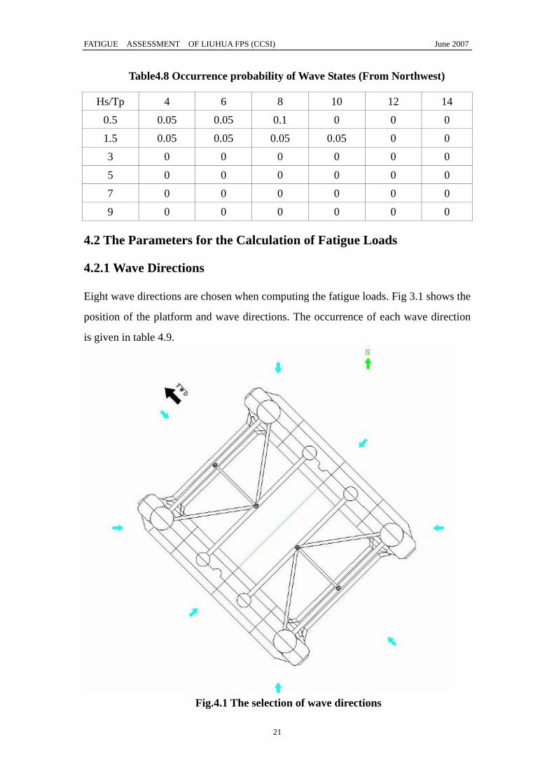
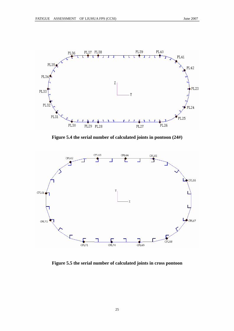
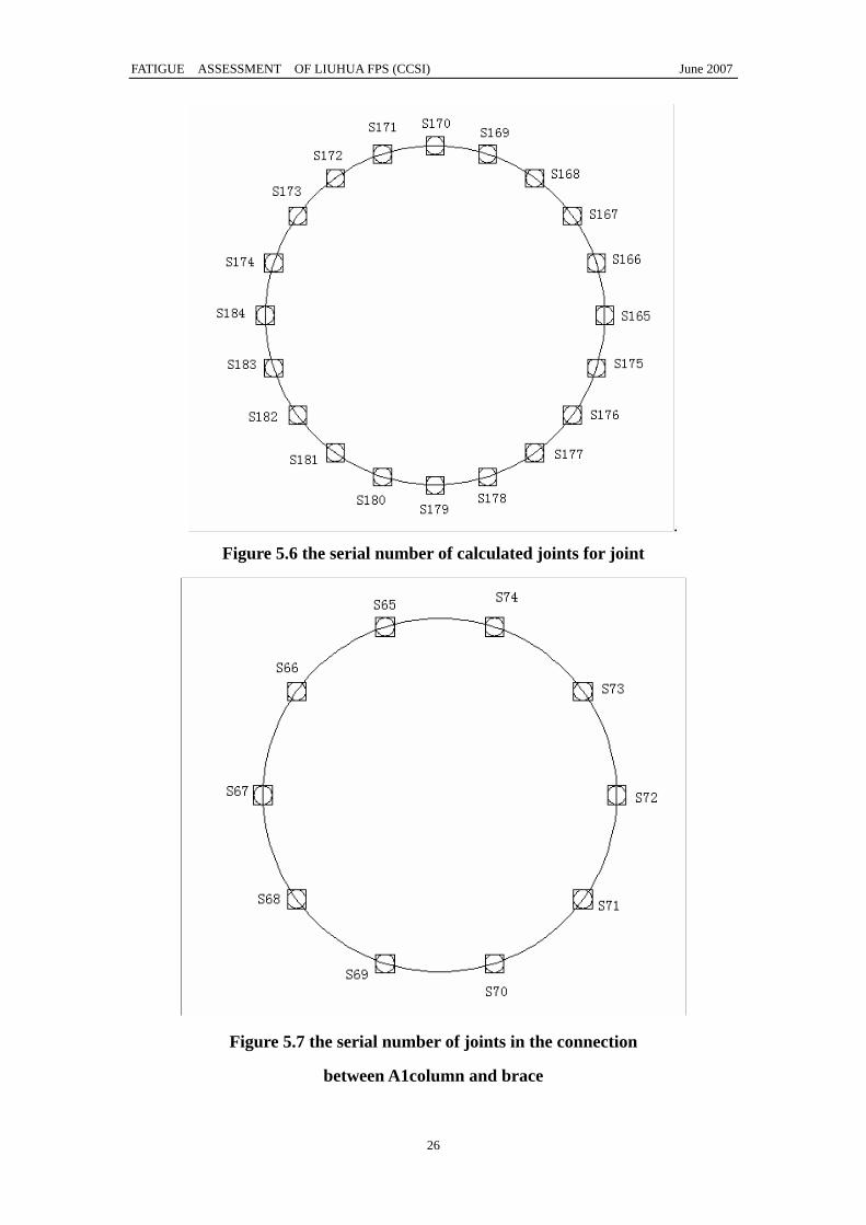
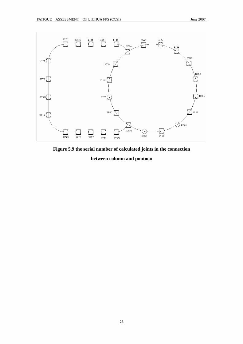
5 Selections of the Joints for Fatigue Assessment 5.1 Selection of the Joint Structures for Fatigue Assessment
According to the ABS rules, GUIDE FOR THE FATIGUE ASSESSMENT OF
OFFSHORE STRUCTURES, 1791 critical joints were selected in the global spectrum
fatigue analysis using coarse mesh FE model. It includes all kinds of fatigable joints
such as the connection between stiffeners and main girders, deck and columns,
pontoons and columns, little stiffeners and strings in the pontoon and columns etc.
nominal stress method was adopted in dealing with the fatigue assessment. After
transforming the fatigue damage into fatigue life, the joints whose fatigue life was less
than 300 years were selected to be meshed fine in order to calculate their fatigue life
exactly and the hot spot stress method was used in calculation. The location and the
number of the joints were list following(the whole joints were list in Appendix A)
Figure 5.1 the numbers of connection between girders
FATIGUE ASSESSMENT OF LIUHUA FPS (CCSI) June 2007
24
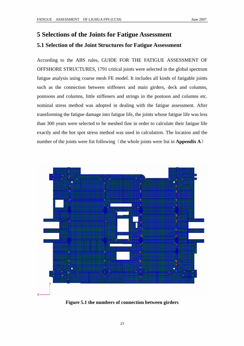
Figure 5.2 the serial number of calculated joints on main deck (partial)
Figure 5.3 the serial number of calculated joints in A4 column (65’ ft)
FATIGUE ASSESSMENT OF LIUHUA FPS (CCSI) June 2007
25
Figure 5.4 the serial number of calculated joints in pontoon (24#)
Figure 5.5 the serial number of calculated joints in cross pontoon
FATIGUE ASSESSMENT OF LIUHUA FPS (CCSI) June 2007
26
. Figure 5.6 the serial number of calculated joints for joint
Figure 5.7 the serial number of joints in the connection
between A1column and brace

FATIGUE ASSESSMENT OF LIUHUA FPS (CCSI) June 2007
27
Figure 5.8 the serial number of calculated joints in the K_joint
between B1column and B4column
FATIGUE ASSESSMENT OF LIUHUA FPS (CCSI) June 2007
28
Figure 5.9 the serial number of calculated joints in the connection
between column and pontoon
FATIGUE ASSESSMENT OF LIUHUA FPS (CCSI) June 2007
29
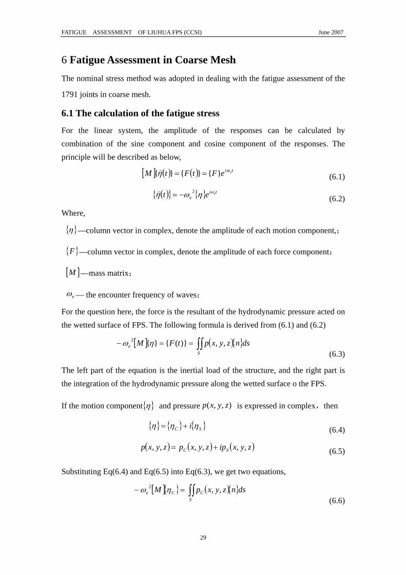
6 Fatigue Assessment in Coarse Mesh The nominal stress method was adopted in dealing with the fatigue assessment of the
1791 joints in coarse mesh.
6.1 The calculation of the fatigue stress
For the linear system, the amplitude of the responses can be calculated by combination of the sine component and cosine component of the responses. The principle will be described as below,
[ ] ( ) ( ) ti eeFtFtM ϖη }{}{}{ ==&& (6.1)
( ){ } { } tie
eet ωηωη 2−=&& (6.2)
Where,
{ }η —column vector in complex, denote the amplitude of each motion component,;
{ }F —column vector in complex, denote the amplitude of each force component;
[ ]M —mass matrix;
eω — the encounter frequency of waves;
For the question here, the force is the resultant of the hydrodynamic pressure acted on the wetted surface of FPS. The following formula is derived from (6.1) and (6.2)
[ ] ( ){ }dsnzyxptFMS
e ∫∫==− ,,)}({}{2 ηω (6.3)
The left part of the equation is the inertial load of the structure, and the right part is the integration of the hydrodynamic pressure along the wetted surface o the FPS.
If the motion component{ }η and pressure ),,( zyxp is expressed in complex,then
{ } { } { }SC i ηηη += (6.4)
( ) ( ) ( )zyxipzyxpzyxp SC ,,,,,, += (6.5)
Substituting Eq(6.4) and Eq(6.5) into Eq(6.3), we get two equations,
[ ]{ } ( ){ }dsnzyxpMS
CCe ∫∫=− ,,2 ηω (6.6)

FATIGUE ASSESSMENT OF LIUHUA FPS (CCSI) June 2007
30
[ ]{ } ( ){ }dsnzyxpMS
SSe ∫∫=− ,,2 ηω (6.7)
For the linear system of wave and FPS, the response of stress is linear. So, the cosine component of the stress is obtained with Eq(6.6), and sine component with Eq(6.7).
The resultant stress may be expressed as sc iσσσ += in complex, consequently, the
amplitude of the stress can be calculated by 22scA σσσ += .
In order to get the corresponding stress response cσ and sσ , the above process is
carried out at different frequency by applying the real and imaginary component of
the loads induced by unit height wave. And then, the amplitude of the stress Aσ is
calculated. Because the calculation is done relative to wave direction and frequency, the transfer function of the stress can be expressed as:
),(),( θωσθωσ eAeH = (6.8)
According to the previous discussion, the total number of the calculation is 1(loading condition number)×8(sea direction number)×15(frequency number)×2(sine component and cosine component)=240.
6.2 Thickness Adjustment
According to the ABS rules, the basic design S-N cures are applicable to the thickness
that do not exceed the reference thickness Rt =22 mm(7/8 inch). For the members
with greater thickness, the thickness correction is to be considered for fatigue strength assessment of welded joint. The following formula applies:
q
Rf t
tSS −⋅= )( (6.9)
Where, S ——unmodified stress range in the S-N curve
t ——plate thickness of the member under assessment
tR——reference thickness (=22mm)
q ——thickness exponent factor (=0.25)

FATIGUE ASSESSMENT OF LIUHUA FPS (CCSI) June 2007
31
6.3 The calculation of the cumulative fatigue damage
6.3.1 The principle of the cumulative fatigue damage calculation
6.3.1.1 The short-term stress-range distribution
The long-term distribution of the sea waves is generally regarded as the combination
of many short-term distributions of the sea waves in shipbuilding and marine
engineering. For each short-term sea state, the wave can be treated as a steady normal
random process, and so do the stress response at the sea state. According to the
statistic property of the steady normal random process, the short-term stress range
distribution for each short-term sea state may be described in continuous probability
density function
In practice, the cyclic stress process for each sea state and sea directionθ is
considered as a steady narrow-banded random process with zero-expectation and the
Rayleigh probability density function can be used to describe the distribution of the
stress amplitude:
⎟⎟⎠
⎞⎜⎜⎝
⎛−= 2
2
2 2exp)(
XXY
yyyfσσ +∞<≤ y0 (6.10)
Where y —Stress amplitude
Xσ —Root-mean-square value of y
Assume the stress energy spectrum at sea directionθ is ),( θωeXXG , it can be
obtained by scaling the wave energy spectrum in the following manner:
),(),(),( 2 θωθωθω ηησ eeeXX GHG ⋅= (6.11)
Where
),( θωσ eH —The stress transfer function
eω —The encounter frequency of waves,
θ —Wave direction,
),( θωηη eG —The spectrum described by encounter frequency, expressed in the
following formula (6.12),
FATIGUE ASSESSMENT OF LIUHUA FPS (CCSI) June 2007
32
θωω
θω ηηηη
cos21
)(),(
gU
GG e
+=
(6.12)
Where,
( )ωηηG —The Pierson-Moskowitz spectrum described by significant wave
height SH and the zero crossing period ZT , as expressed in Eq(6.13)
( )⎟⎟
⎠
⎞
⎜⎜
⎝
⎛⎟⎟⎠
⎞⎜⎜⎝
⎛−⎟⎟
⎠
⎞⎜⎜⎝
⎛= −− 4
45
42 21exp24
ωππ
ωππ
ωηηZZ
S
TTH
G (6.13)
PZ TT 772.0= (6.14)
PT —amplitude period
The 0-th 0m and second order 2m spectral moments are calculated as follows:
∫+∞
=0
),( eeXXn
en dGm ωθωω (n= 0, 2) (6.15)
The root-mean-square value of the cyclic stress process can be achieved in the following formula,
00
)( mdGXXX == ∫+∞
ωωσ (6.16)
In addition, to get the number of the stress cycles in a certain time, the zero-up crossing frequency needs to be calculated as follows,
0
20 2
1mmf
π=
(6.17)
When the cyclic stress process is a narrow-banded process, the stress range S and the stress amplitude y can be expressed as follows:
yS 2= or 2/Sy = (6.18)
Hence, the probability density function of the stress range is derived from Eq(6.10) and Eq(6.17) in the following formula:
⎟⎟⎠
⎞⎜⎜⎝
⎛−= 2
2
2 8exp
4)(
XXS
SSSfσσ +∞<≤ S0 (6.19)
6.3.1.2 The calculation of the cumulative fatigue damage When the fatigue load spectrum is expressed in continuous probability density
FATIGUE ASSESSMENT OF LIUHUA FPS (CCSI) June 2007
33
function, the cumulative fatigue damage can be calculated as follows:
∫ ∫∫+∞+∞
===L
SL
SL dSN
SfN
NdSSfN
NdnD
00
)()(
(6.20)
Where S— Stress range,
)(SfS — Probability density function of the stress range distribution,
N— Average number of loading cycles to failure under constant amplitude loading at that stress range according to the relevant S-N curve,
LN —The total number of stress cycles,
dSSfNdn SL )(= — The number of stress cycles between S and S+dS,
∫L — The integration in the total period of time.
In calculation, the relation between the number of loading cycles to failure and the relevant constant stress amplitude in Eq(6.10) needs to be known and generally is expressed in S-N curves as follows:
ANS m = (6.21)
Where
m 、 A — S-N curve constant
Substituting (6.20) into (6.19), then we gets the cumulative fatigue damage formula:
∫+∞
=0
)( dSSfSA
ND SmL
(6.22)
Assuming the voyage time for i-th sea state and j-th sea direction is ijT , then the
damage in this period of time may be calculated in the following formula :
∫+∞
=0
0 )( dSSfSAfT
D Sijmijij
ij
(6.23)
Where
ijf0 —Zero-up crossing frequency of the cyclic stress process, which can be
obtained by Eq(6.19);
ijij fT 0⋅ —The number of the stress cycles in the period ijT ;

FATIGUE ASSESSMENT OF LIUHUA FPS (CCSI) June 2007
34
)(SfSij —The short-term stress range distribution in the period ijT .
Substituting the expression (6.15) for the short-term stress range distribution )(SfSij ,
we get
( ) )2
1(220 mAfT
Dm
Xijijij
ij +Γ= σ=
( ) )2
1(22 00 mm
AfT m
ijijij +Γ
(6.24)
Where
Xijσ —Root-mean-square value of the cyclic stress process, given by Eq(6.6)
ijm0 —zero order moment of the stress energy spectrum
)( Γ —Gamma function.
Assuming T is the period of the long-term distribution, the relevant long-term
stress-range distribution is consisted of Sn sea states and the corresponding
occurrence probability is ip for each sea state. The number of the wave directions is
subdivided into Hn and the occurrence probability is jp for each wave direction,
then jiij ppTT ⋅⋅= , we get the total cumulative fatigue damage in the period T as
follows:
∑∑= =
=S Hn
i
n
jijT DD
1 1 =( )mij
n
i
n
ijji mfppmAT S H
01
0 22)2
1( ∑∑=
+Γ (6.25)
The cumulative fatigue damage of the structure should satisfy the following demand in the design life,
0.1≤TD (6.26)
6.4 Selection of S-N curves
The correct S-N curve was selected for each calculated join according to the section 3
of the 《 GUIDE FOR THE FATIGUE ASSESSMENT OF OFFSHORE
STRUCTURES》,the results was list in Appendix C.
6.5 The Results of Fatigue Assessment in Coarse Mesh
According to the theory above-mentioned and ABS rules, the fatigue accumulated
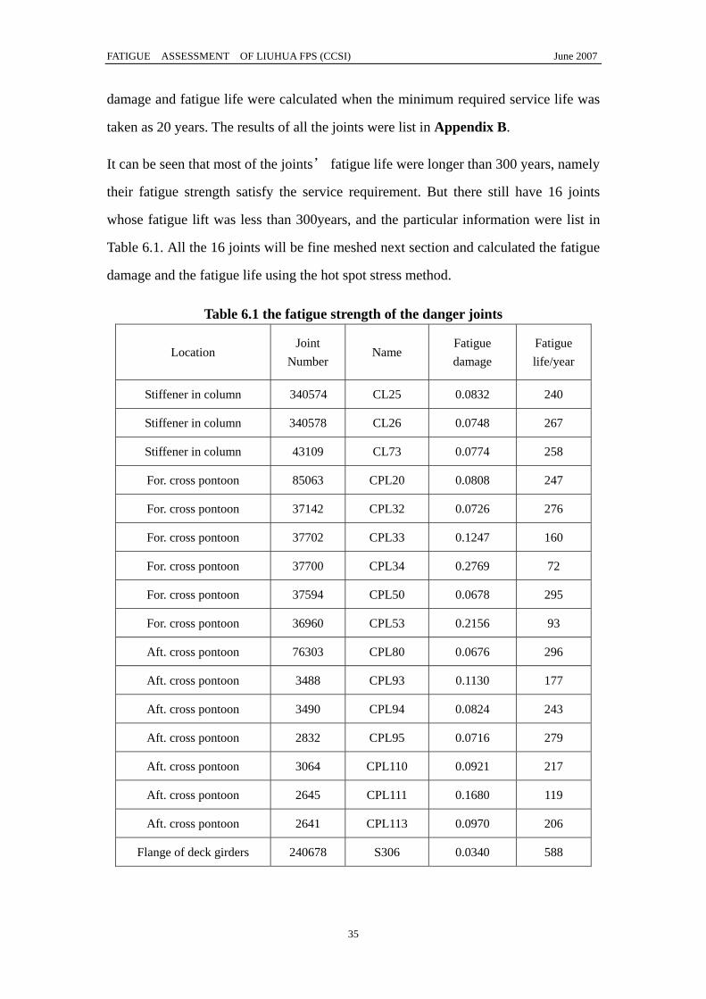
FATIGUE ASSESSMENT OF LIUHUA FPS (CCSI) June 2007
35
damage and fatigue life were calculated when the minimum required service life was
taken as 20 years. The results of all the joints were list in Appendix B.
It can be seen that most of the joints’ fatigue life were longer than 300 years, namely
their fatigue strength satisfy the service requirement. But there still have 16 joints
whose fatigue lift was less than 300years, and the particular information were list in
Table 6.1. All the 16 joints will be fine meshed next section and calculated the fatigue
damage and the fatigue life using the hot spot stress method.
Table 6.1 the fatigue strength of the danger joints
Location Joint
Number Name
Fatigue damage
Fatigue life/year
Stiffener in column 340574 CL25 0.0832 240
Stiffener in column 340578 CL26 0.0748 267
Stiffener in column 43109 CL73 0.0774 258
For. cross pontoon 85063 CPL20 0.0808 247
For. cross pontoon 37142 CPL32 0.0726 276
For. cross pontoon 37702 CPL33 0.1247 160
For. cross pontoon 37700 CPL34 0.2769 72
For. cross pontoon 37594 CPL50 0.0678 295
For. cross pontoon 36960 CPL53 0.2156 93
Aft. cross pontoon 76303 CPL80 0.0676 296
Aft. cross pontoon 3488 CPL93 0.1130 177
Aft. cross pontoon 3490 CPL94 0.0824 243
Aft. cross pontoon 2832 CPL95 0.0716 279
Aft. cross pontoon 3064 CPL110 0.0921 217
Aft. cross pontoon 2645 CPL111 0.1680 119
Aft. cross pontoon 2641 CPL113 0.0970 206
Flange of deck girders 240678 S306 0.0340 588
FATIGUE ASSESSMENT OF LIUHUA FPS (CCSI) June 2007
36
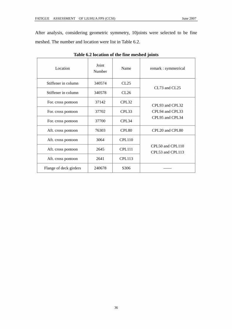
After analysis, considering geometric symmetry, 10joints were selected to be fine
meshed. The number and location were list in Table 6.2.
Table 6.2 location of the fine meshed joints
Location Joint
Number Name remark : symmetrical
Stiffener in column 340574 CL25
Stiffener in column 340578 CL26 CL73 and CL25
For. cross pontoon 37142 CPL32
For. cross pontoon 37702 CPL33
For. cross pontoon 37700 CPL34
CPL93 and CPL32 CPL94 and CPL33 CPL95 and CPL34
Aft. cross pontoon 76303 CPL80 CPL20 and CPL80
Aft. cross pontoon 3064 CPL110
Aft. cross pontoon 2645 CPL111
Aft. cross pontoon 2641 CPL113
CPL50 and CPL110 CPL53 and CPL113
Flange of deck girders 240678 S306 ——
FATIGUE ASSESSMENT OF LIUHUA FPS (CCSI) June 2007
37
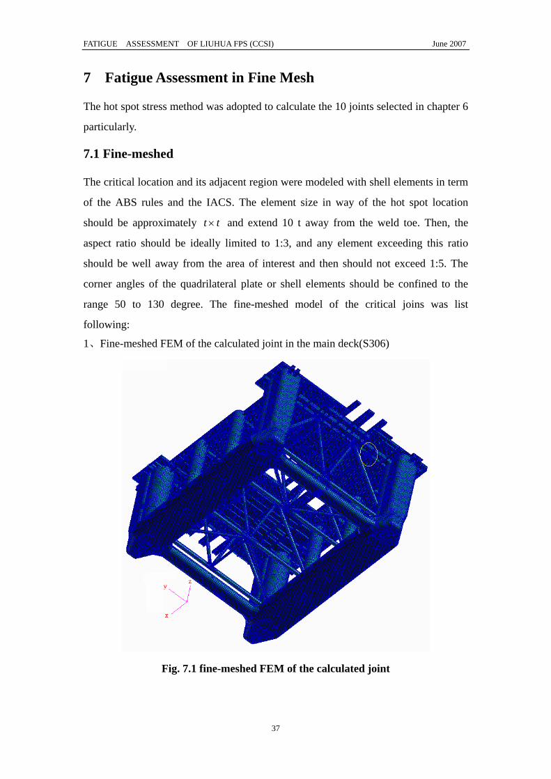
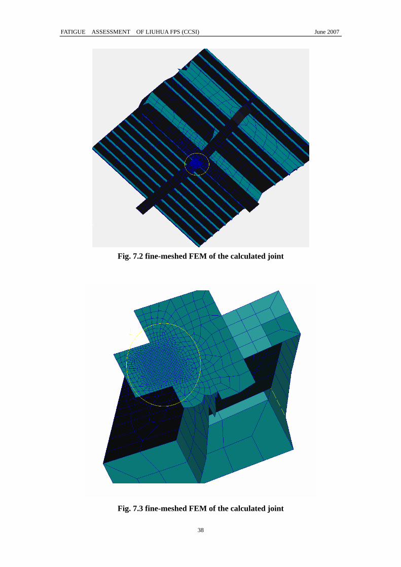
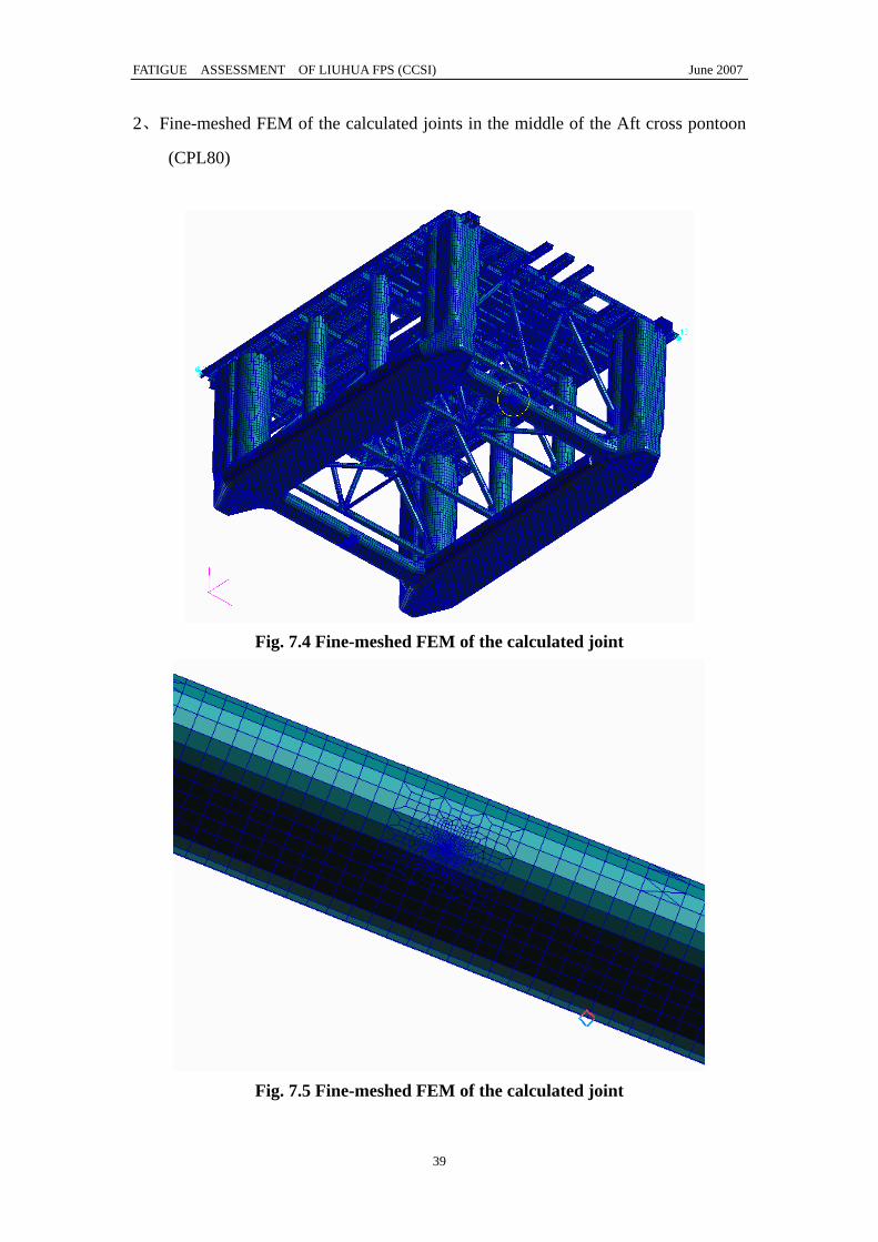
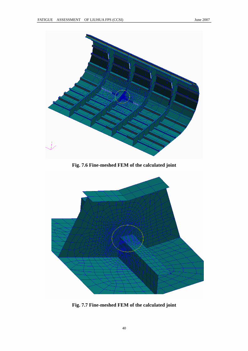
7 Fatigue Assessment in Fine Mesh
The hot spot stress method was adopted to calculate the 10 joints selected in chapter 6
particularly.
7.1 Fine-meshed
The critical location and its adjacent region were modeled with shell elements in term
of the ABS rules and the IACS. The element size in way of the hot spot location
should be approximately tt × and extend 10 t away from the weld toe. Then, the
aspect ratio should be ideally limited to 1:3, and any element exceeding this ratio
should be well away from the area of interest and then should not exceed 1:5. The
corner angles of the quadrilateral plate or shell elements should be confined to the
range 50 to 130 degree. The fine-meshed model of the critical joins was list
following:
1、Fine-meshed FEM of the calculated joint in the main deck(S306)
Fig. 7.1 fine-meshed FEM of the calculated joint
FATIGUE ASSESSMENT OF LIUHUA FPS (CCSI) June 2007
38
Fig. 7.2 fine-meshed FEM of the calculated joint
Fig. 7.3 fine-meshed FEM of the calculated joint
FATIGUE ASSESSMENT OF LIUHUA FPS (CCSI) June 2007
39
2、Fine-meshed FEM of the calculated joints in the middle of the Aft cross pontoon
(CPL80)
Fig. 7.4 Fine-meshed FEM of the calculated joint
Fig. 7.5 Fine-meshed FEM of the calculated joint
FATIGUE ASSESSMENT OF LIUHUA FPS (CCSI) June 2007
40
Fig. 7.6 Fine-meshed FEM of the calculated joint
Fig. 7.7 Fine-meshed FEM of the calculated joint

FATIGUE ASSESSMENT OF LIUHUA FPS (CCSI) June 2007
41
3、Fine-meshed FEM of the calculated joints in the connection between pontoon and
cross pontoon(CPL110,CPL111,CPL113).
Fig. 7.8 Fine-meshed FEM of the calculated joints
Fig. 7.9 Fine-meshed FEM of the calculated joints
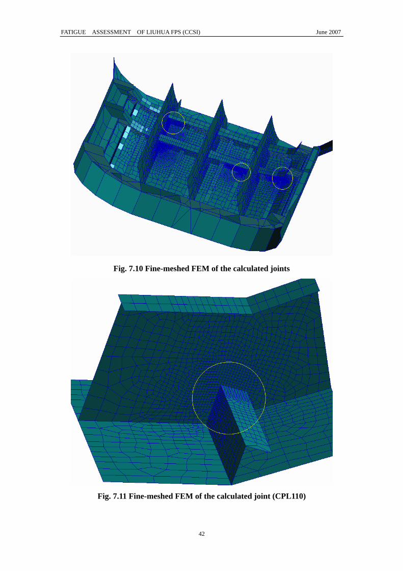
FATIGUE ASSESSMENT OF LIUHUA FPS (CCSI) June 2007
42
Fig. 7.10 Fine-meshed FEM of the calculated joints
Fig. 7.11 Fine-meshed FEM of the calculated joint (CPL110)

FATIGUE ASSESSMENT OF LIUHUA FPS (CCSI) June 2007
43
Fig. 7.12 Fine-meshed FEM of the calculated joint(CPL111)
Fig. 7.13 Fine-meshed FEM of the calculated joint(CPL113)

FATIGUE ASSESSMENT OF LIUHUA FPS (CCSI) June 2007
44
4、Fine-meshed FEM of the calculated joints in the For. Cross pontoon (CPL32,
CPL33 and CPL34)
Fig. 7.14 Fine-meshed FEM of the calculated joints
Fig. 7.15 Fine-meshed FEM of the calculated joints

FATIGUE ASSESSMENT OF LIUHUA FPS (CCSI) June 2007
45
Fig. 7.16 Fine-meshed FEM of the calculated joints
Fig. 7.17 Fine-meshed FEM of the calculated joint (CPL 32)
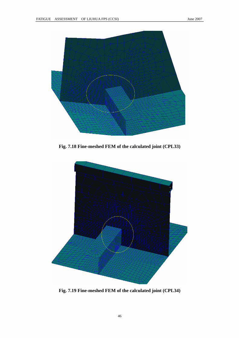
FATIGUE ASSESSMENT OF LIUHUA FPS (CCSI) June 2007
46
Fig. 7.18 Fine-meshed FEM of the calculated joint (CPL33)
Fig. 7.19 Fine-meshed FEM of the calculated joint (CPL34)
FATIGUE ASSESSMENT OF LIUHUA FPS (CCSI) June 2007
47
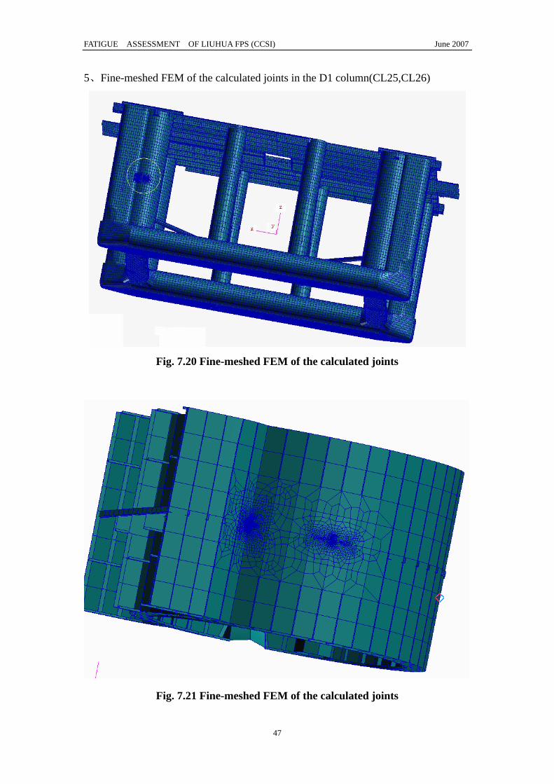
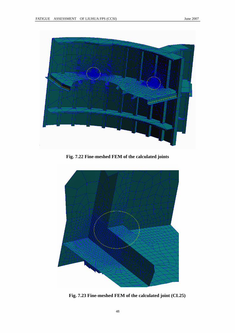
5、Fine-meshed FEM of the calculated joints in the D1 column(CL25,CL26)
Fig. 7.20 Fine-meshed FEM of the calculated joints
Fig. 7.21 Fine-meshed FEM of the calculated joints
FATIGUE ASSESSMENT OF LIUHUA FPS (CCSI) June 2007
48
Fig. 7.22 Fine-meshed FEM of the calculated joints
Fig. 7.23 Fine-meshed FEM of the calculated joint (CL25)

FATIGUE ASSESSMENT OF LIUHUA FPS (CCSI) June 2007
49
Fig. 7.24 Fine-meshed FEM of the calculated joint (CL26)
7.2 The area of crack likely arising
For fatigue node of stress centralizing, the areas where crack may arise are not sure. A
detail explanation for three different structure types of 10 refined nodes will be given.
1) Angle steel perforates round frame or bulkhead,see Figure 7.25. The 9 parts
signed in figure all will come forth with crack. By calculation and analysis of
node stress, we got that the stresses of NO.2, NO.4, NO.6, NO.7, NO.8 and NO. 9
are smaller than others, so their fatigue damages are relatively small. The stresses
of NO.1, NO.2, NO.3, NO.4 and NO.5 are calculated in this assessment.
2) The node on the intersection of two angle steels, which has a 90 degree angle, see
Figure 7.26. The stresses of the 4 parts signed in the figure will be calculated.

FATIGUE ASSESSMENT OF LIUHUA FPS (CCSI) June 2007
50
Figure7.25 Figure of crack arising
Figure7.26 Figure of crack arising
FATIGUE ASSESSMENT OF LIUHUA FPS (CCSI) June 2007
51
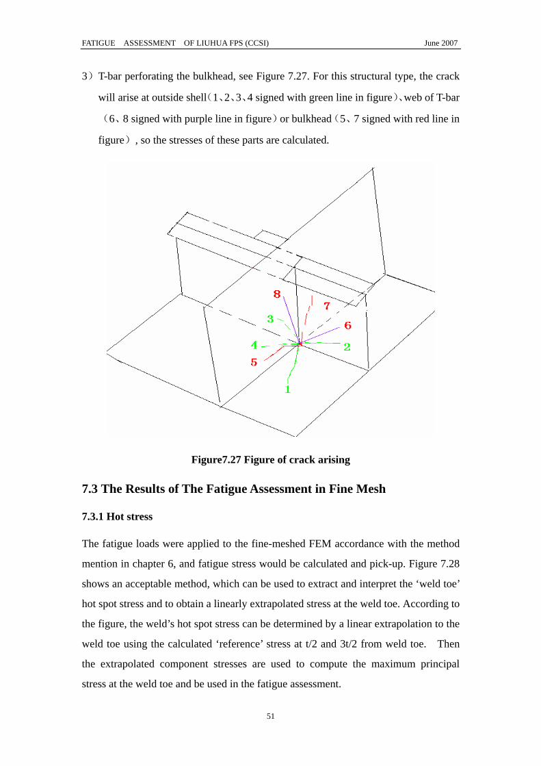
3)T-bar perforating the bulkhead, see Figure 7.27. For this structural type, the crack
will arise at outside shell(1、2、3、4 signed with green line in figure)、web of T-bar
(6、8 signed with purple line in figure)or bulkhead(5、7 signed with red line in
figure), so the stresses of these parts are calculated.
Figure7.27 Figure of crack arising
7.3 The Results of The Fatigue Assessment in Fine Mesh
7.3.1 Hot stress
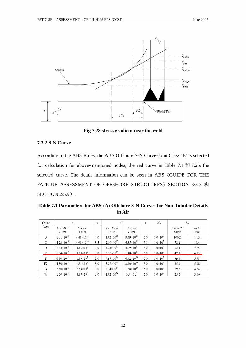
The fatigue loads were applied to the fine-meshed FEM accordance with the method
mention in chapter 6, and fatigue stress would be calculated and pick-up. Figure 7.28
shows an acceptable method, which can be used to extract and interpret the ‘weld toe’
hot spot stress and to obtain a linearly extrapolated stress at the weld toe. According to
the figure, the weld’s hot spot stress can be determined by a linear extrapolation to the
weld toe using the calculated ‘reference’ stress at t/2 and 3t/2 from weld toe. Then
the extrapolated component stresses are used to compute the maximum principal
stress at the weld toe and be used in the fatigue assessment.
FATIGUE ASSESSMENT OF LIUHUA FPS (CCSI) June 2007
52
Fig 7.28 stress gradient near the weld
7.3.2 S-N Curve
According to the ABS Rules, the ABS Offshore S-N Curve-Joint Class ‘E’ is selected
for calculation for above-mentioned nodes, the red curve in Table 7.1 和 7.2is the
selected curve. The detail information can be seen in ABS《GUIDE FOR THE
FATIGUE ASSESSMENT OF OFFSHORE STRUCTURES》SECTION 3/3.3 和
SECTION 2/5.9).
Table 7.1 Parameters for ABS-(A) Offshore S-N Curves for Non-Tubular Details in Air

FATIGUE ASSESSMENT OF LIUHUA FPS (CCSI) June 2007
53
Table 7.2 Parameters for ABS-(CP) Offshore S-N Curves for Non-Tubular
Details in Seawater with Cathodic Protection
7.3.3 The Results of the Fatigue Assessment in Fine Mesh According to ABS Rules, for those cases where an existing structure is being reused
or converted, the basis of the fatigue assessment should be modified to reflect past
service or previously accumulated fatigue damage. If pD denotes the damage from
past service,α is a factor to reflect the uncertainty with which the past service data
are known, the ‘unused fatigue damage’, RΔ , may be taken as:
FDFDpR /)1( α⋅−=Δ (7.1)
Where, FDF is the fatigue design factor. According to the fatigue guide, for the
critical structure details above water such as integral deck, FDF was taken as 3, while
for the ordinary structure be 2; for the critical structure details in water or submerged
such as column stabilized, FDF was taken as 5, while for the ordinary structure be 3.
But the minimum Factor to be applied to uninspected ‘critical’ or uninspected
‘ordinary’ structure details is 10 or 5, respectively. In this assessment, the FDF was
taken as 5.
For the uncertainty factorα , when the past service data are well documented, α
may be taken as 1.0, otherwise a higher value should be used. So the assessment
formula was taken as
RD Δ≤ (7.2)
Where,

FATIGUE ASSESSMENT OF LIUHUA FPS (CCSI) June 2007
54
D——cumulative fatigue damage
In this assessment, the uncertainty factor α was taken as 1.50 foe the past service
data was not well documented. And the past service damage pD was calculated from
analysis,
pdp TTDD ⋅= )/( (7.3)
Where,
PT ——the past service life,taken as 31 accordance with the data;
dT ——design life,taken as 20 years。
Figure 7.29~7.38 will show the 10 joints’ (CPL80、CPL110、CPL111、CPL113、
CPL32、CPL33、CPL34、CL25、CL26、S306) RAOs under different wave direction
and different frequency, and they are corresponding to the part 1 in Figure 7.25, part 3
in Figure 7.26 and part 8 in Figure 7.27.Other stress transfer function was list in
Appendix D.
Figure 7.29 the stress transfer function of the calculated joint (CPL80)

FATIGUE ASSESSMENT OF LIUHUA FPS (CCSI) June 2007
55
Figure 7.30 the stress transfer function of the calculated joint (CPL110)
Figure 7.31 the stress transfer function of the calculated joint (CPL111)

FATIGUE ASSESSMENT OF LIUHUA FPS (CCSI) June 2007
56
Figure 7.32 the stress transfer function of the calculated joint (CPL121)
Figure 7.33 the stress transfer function of the calculated joint (CPL32)

FATIGUE ASSESSMENT OF LIUHUA FPS (CCSI) June 2007
57
Figure 7.34 the stress transfer function of the calculated joint (CPL33)
Figure 7.35 the stress transfer function of the calculated joint (CPL34)

FATIGUE ASSESSMENT OF LIUHUA FPS (CCSI) June 2007
58
Figure 7.36 the stress transfer function of the calculated joint (CL25)
Figure 7.37 the stress transfer function of the calculated joint (CL26)

FATIGUE ASSESSMENT OF LIUHUA FPS (CCSI) June 2007
59
Figure 7.38 the stress transfer function of the calculated joint (S306)
The 10 joints’ fatigue damage was calculated in term of the theoretic mentioned above.
Due to differences of structures, the results are given respectively. The Table 7.3 is
corresponding to the parts given by Figure 7.25, but the CPL121 is corresponding to
the part given in Figure 7.27(the limit is 50 years); the Table 7.4 is corresponding to
the parts given by Figure 7.26 (the limit is 50 years).
Table 7.3 fatigue accumulated damage of the dangerous joins
Location Joints Number
Joints Name
Residual
fatigue
strength
Residual
fatigue
life (year)
Position of
crack
For. cross pontoon (Figure7.14、7.17)
37142 CPL32 0.1114 11.7 1(Figure7.25)
0.1639 42.2 3(Figure7.25)For. cross pontoon (Figure7.14、7.18)
37702 CPL33
0.1638 42.1 5(Figure7.25)
0.1066 10.6 1(Figure7.25)
0.1595 36.6 3(Figure7.25)For. cross pontoon (Figure7.14、7.19)
37700 CPL34
0.1591 36.1 5(Figure7.25)
FATIGUE ASSESSMENT OF LIUHUA FPS (CCSI) June 2007
60
Aft. Cross pontoon (Figure7. 4、7. 7)
76303 CPL80 0.1130 12.1 1(Figure7.25)
Aft. Cross pontoon (Figure7.8、7.11)
3064 CPL110 0.1760 68.1 1(Figure7.25)
0.1691 51.0 1(Figure7.25)Aft. Cross pontoon (Figure7.8、7.12)
2645 CPL111 0.1685 49.7 5(Figure7.25)
Aft. Cross pontoon (Figure7.8、7.13)
12338 CPL121 0.136 19.76 8(Figure7.27)
Girders in main deck
(Figure7.1、7.3)
240678 S306 0.116 12.84 1(Figure7.25)
Table 7.3 fatigue accumulated damage of the dangerous joins
Location Joints Number
Joints Name
Residual
fatigue
strength
Residual
fatigue
life (year)
Position of
crack
0.1741 62.5 1(Figure7.26)
0.1194 13.8 3(Figure7.26)
Stiffener in A1 column
(Figure7.14、7.17)
340574 CL25
0.1140 12.3 4(Figure7.26)
0.1254 15.6 2(Figure7.26)
0.15 27.60 3(Figure7.26)
Stiffener in A1 column
(Figure7.14、7.17)
340578 CL26
0.1667 46.5 4(Figure7.26)

FATIGUE ASSESSMENT OF LIUHUA FPS (CCSI) June 2007
61
8 Conclusions and suggestions of fatigue assessment
The platform for this assessment has been using for 31 years. There are a lot of
tubular joints, intersections between girders, nodes of angle plate perforating the
bulkhead and so on. Under repeating loads, these nodes are easy to raise fatigue
damage, so we do fatigue assessment for these nodes.
According to the results of fatigue assessment, it can be got that the fatigue lives of
most nodes are relatively large; only some nodes’ fatigue strength in local areas is
relatively weak. These nodes are shown as below:
1)The connection between the stringer stiffener and the ring stiffener in For.
Crosspontoon and the Aft. Crosspontoon (CPL33, CPL34, CPL94, CPL95), see
Figure 8.1; the connection between the stringer stiffener and the ring stiffener in
Aft. Cross pontoon and the Aft. Cross pontoon (CPL110, CPL111 and CPL53) and
so on. Because the cross pontoons are used as ballast tank and eroded by sea water
in service period, these accelerate the fatigue of the structures. Meanwhile, more
attention should be paid to other nodes.
Figure 8.1 the location of the fatigue joints in crosspontoons

FATIGUE ASSESSMENT OF LIUHUA FPS (CCSI) June 2007
62
2)The joints in D1 and A1 columns (such as CL25,CL26,CL73), see Figure 8.2,
because the rigidity of the local structure is relatively strong, the fatigue damage
would be great. Therefore, new brackets should be added in order to reduce the
stress concentration (see Figure 8.3). The same method can be used to the
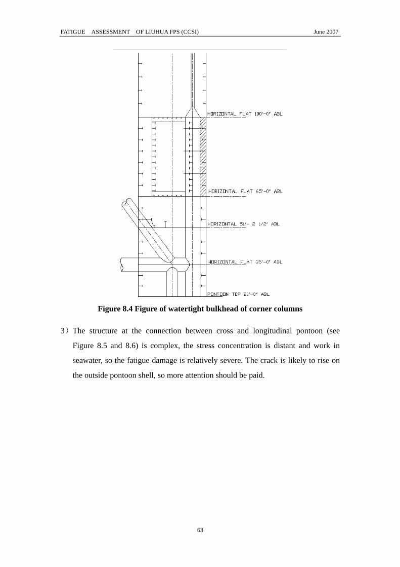
watertight bulkheads of the 4 corner columns (EL35’、EL51’—2(1/2)”、EL65’、
EL100’, see Figure 8.4) in order to reduce the stress concentration.
Figure 8.2 the location of the fatigue joints in columns
Figure 8.3 weld position of bracket and
FATIGUE ASSESSMENT OF LIUHUA FPS (CCSI) June 2007
63
Figure 8.4 Figure of watertight bulkhead of corner columns
3)The structure at the connection between cross and longitudinal pontoon (see
Figure 8.5 and 8.6) is complex, the stress concentration is distant and work in
seawater, so the fatigue damage is relatively severe. The crack is likely to rise on
the outside pontoon shell, so more attention should be paid.

FATIGUE ASSESSMENT OF LIUHUA FPS (CCSI) June 2007
64
Figure 8.5 the location of fatigue joints in the connection
between pontoon and crosspontoon
Figure 8.6 Figure of the connection of longitudinal pontoon
4)The stress concentration is distant at the connection between deck girders (see
Figure 8.7), so the fatigue damage is relatively severe. Therefore, new brackets
should be added in order to reduce the stress concentration (see Figure 8.8) and
enhance the fatigue life. During service period, deck structure should be examined
regularly.

FATIGUE ASSESSMENT OF LIUHUA FPS (CCSI) June 2007
65
Figure 8.7 location of the connection between deck girders
Figure 8.8 Figure of the connection of the deck girders
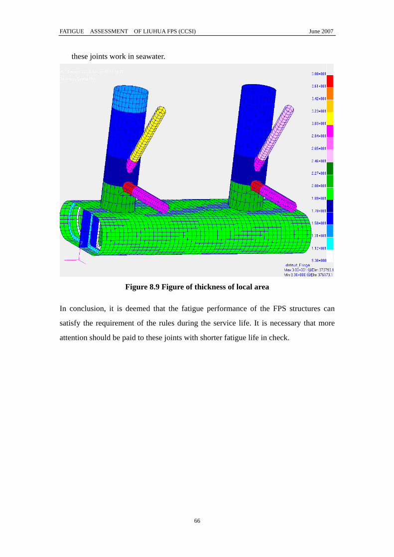
5)Because of using high strength steel(ABS_AH32) and enhancing the thickness (see
Figure 8.9), so the stresses of tubular joints are relatively low. The fatigue
performance of the tubular joints satisfies the requirement of the rules during the
service life. But the attentions also should be paid to some tubular joints, because
FATIGUE ASSESSMENT OF LIUHUA FPS (CCSI) June 2007
66
these joints work in seawater.
Figure 8.9 Figure of thickness of local area
In conclusion, it is deemed that the fatigue performance of the FPS structures can
satisfy the requirement of the rules during the service life. It is necessary that more
attention should be paid to these joints with shorter fatigue life in check.


![Effects of part build orientations on fatigue behaviour of ... · fatigue data. Lee and Huang [8] have investigated the fatigue data for several print orientations of ABS and ABSplus](https://static.fdocuments.us/doc/165x107/5e931ffbab839750302369bf/effects-of-part-build-orientations-on-fatigue-behaviour-of-fatigue-data-lee.jpg)