1 Foundations of Software Design Fall 2002 Marti Hearst Lecture 18: Hash Tables.

1

Foundations of Software DesignFall 2002Marti Hearst

Lecture 18: Hash Tables

2

Unresolved Question on Heaps

• Q: What happens if there is more than one item to swap with?

• A: Swap with the larger one.

3Slide copyright 1999 Addison Wesley Longman

Move the last node onto the root.

19

4222135

23

45

42

27

Removing the Top of the Heap



Push the out-of-place node downward, swapping with its larger child until the new node reaches an acceptable location.

19

4222135

23

27

42




19

4222135

23

42

27




19

4222127

23

42

35

7

Hash Tables

• Very useful data structure– Good for storing and retrieving key/value pairs

• Often in constant time!– Not good for iterating through a list of items

• Example applications:– Storing posting lists in Information Retrieval

• For each word, a list of which documents it occurs in• This assumes you will not be looking up words in

alphabetical order– Storing objects according to ID numbers

• When the ID numbers are widely spread out• When you don’t need to access items in ID order

8Slide adapted from lecture by Andreas Veneris

• How can you store all Social security numbers in an array and have O(1) access?

– Use an array with range 0 - 999,999,999

– This will give you O(1) access time but …– …considering there are approx. 32,000,000 people in

Canada you waste 1,000,000,000-32,000,000 array entries!

• Problem: The range of key values we are mapping is too large (0-999,999,999) when compared to the # of keys (American citizens)

Why Not Arrays?


Hash Tables

• We want a data structure that, given a collection of n keys, implements the dictionary operations Insert(), Delete() and Search() efficiently.

• Binary search trees: can do that in O(log n) time and are space efficient.

• Arrays: can do this in O(1) time but they are not space efficient.

• Hash Tables: A generalization of an array that under some reasonable assumptions is O(1) for Insert/Delete/Search of a key


• Hash Tables solve this problem by using a much smaller array and mapping keys with a hash function.

• Let universe of keys U and an array of size m. A hash

function h is a function from U to 0…m, that is:

h : U 0…m

Hash Tables

U

(universe of keys)

k1 k2

k3 k4 k6

0

1234567

h (k2)=2h (k1)=h (k3)=3

h (k6)=5

h (k4)=7

11

The mod function

• Stands for modulo• When you divide x by y, you get a result and a remainder• Mod is the remainder

– 8 mod 5 = 3– 9 mod 5 = 4– 10 mod 5 = 0– 15 mod 5 = 0

• Thus for A mod M, multiples of M give the same result, 0– But multiples of other numbers do not give the same result– So what happens when M is a prime number?


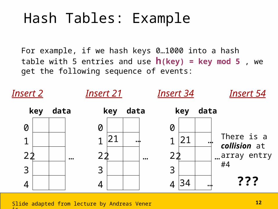
Hash Tables: Example

For example, if we hash keys 0…1000 into a hash table with 5 entries and use h(key) = key mod 5 , we get the following sequence of events:

0

1

2

3

4

key data

Insert 2

2 …

0

1

2

3

4

key data

Insert 21

2 …

21 …0

1

2

3

4

key data

Insert 34

2 …

21 …

34 …

Insert 54

There is a collision atarray entry #4

???


• The problem arises because we have two keys that hash in the same array entry, a collision. There are two ways to resolve collision:

– Hashing with Chaining: every hash table entry contains a pointer to a linked list of keys that hash in the same entry

– Hashing with Open Addressing: every hash table entry contains only one key. If a new key hashes to a table entry which is filled, systematically examine other table entries until you find one empty entry to place the new key

Dealing with Collisions


Hashing with Chaining

The problem is that keys 34 and 54 hash in the same entry (4). We solve this collision by placing all keys that hash in the same hash table entry in a LIFO list (chain or bucket) pointed by this entry:

0

1

2

3

4

other key key data

Insert 54

2

21

54 34

CHAIN

0

1

2

3

4

Insert 101

2

21

54 34

101


• What is the running time to insert/search/delete?

– Insert: It takes O(1) time to compute the hash function and insert at head of linked list

– Search: It is proportional to max linked list length– Delete: Same as search

• Therefore, in the unfortunate event that we have a “bad” hash function all n keys may hash in the same table entry giving an O(n) run-time!

So how can we create a “good” hash function?



• Hash functions are “good” provided that the keys satisfy (approximately) the assumption of:

• Uniform hashing:– each key is equally likely to hash in any

of the m slots (sometimes unrealistic)



Division Method

• Certain values of m may not be good:

– When m = 2p then h(k) is the p lower-order bits

of the key

– Good values for m are prime numbers which are not close to exact powers of 2.

• For example, if you want to store 2000 elements then m=701 (m = hash table length) yields a hash function:

h(k) = k mod m

h(key) = k mod 701


Choosing a Hash Function

• The performance of the hash table depends on a having a hash function which evenly distributes the keys.

• Choosing a good hash function requires taking into account the kind of data that will be used.– The statistics of the key distribution needs to be

accounted for. – E.g., Choosing the first letter of a last name will

cause problems depending on the nationality of the population

• Most programming languages (including java) have hash functions built in.

19Slide adapted from lecture by Hector Garcia-Molina

Rule of thumb:

• Try to keep space utilization (load factor)between 50% and 80%

Load factor = _# keys used___total # slots in table

• If < 50%, wasting space• If > 80%, overflows significant

depends on how good hashfunction is & on # keys/bucket


Hashing with Open Addressing

• So far we have studies hashing with chaining, using a list to store keys that hash to the same location.

• Another option is to store all the keys directly in the table.

• Open addressing– collisions are resolved by systematically

examining other table indexes, i0 , i1 , i2 , … until an empty slot is located.


Open Addressing• The key is first mapped to a slot:

• If there is a collision subsequent probes are performed:

• Linear Probing:– When c=1 the collision resolution is done as a linear

search.

)( index 10 ki h

0formod)(1 jmcii jj

22

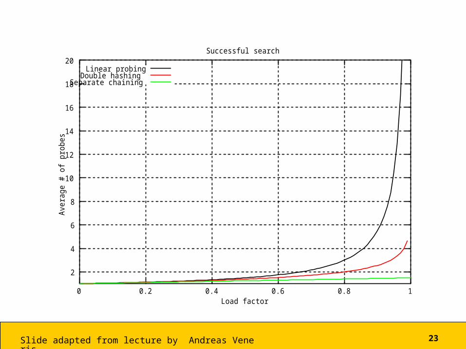
Double Hashing

• Apply a second hash function after the first• We won’t worry about details, but the

following charts show – Double hashing faster than linear probing– But bucket chains faster than double hashing


2

4

6

8

10

12

14

16

18

20

0 0.2 0.4 0.6 0.8 1

Aver

age

# of

pro

bes

Load factor

Successful search

Linear probingDouble hashing

Separate chaining


2

4

6

8

10

12

14

16

18

20

0 0.2 0.4 0.6 0.8 1

Aver

age

# of

pro

bes

Load factor

Unsuccessful search

Linear probingDouble hashing

Separate chaining


• Hashing good for probes given keye.g., SELECT …

FROM RWHERE R.A = 5

Indexing vs Hashing

26

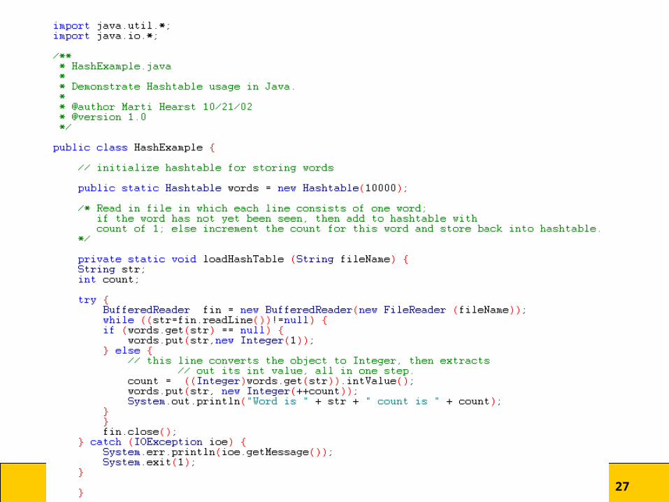
Hash Tables in Java• Java includes a Hashtable class

– In java.util.*• http://java.sun.com/j2se/1.3/docs/api/java/util/Hashtable.html

– Keys are objects; you have to use casting.• As a programmer, you don’t see the collision detection,

chaining, etc• Uses open hashing (chaining)

• You can set – The initial table size– The load factor

• Default is .75

• To change the hash function– Write your own version of Hashtable that extends

java.util.Dictionary• See http://www.cs.utah.edu/classes/cs3510/assignments/assign4/

28

Main

Input File

Output


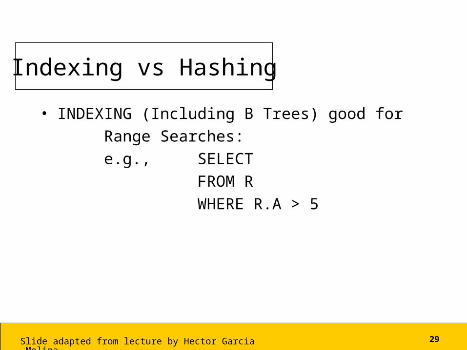
• INDEXING (Including B Trees) good forRange Searches:e.g., SELECT

FROM RWHERE R.A > 5

Indexing vs Hashing

30

Hash Tables vs. Search Trees

• Hash tables great for selecting individual items– Fast search and insert– O(1) if the table size and hash function are chosen

well– Good for access data that is stored on disk

• BUT– Hash trees inefficient for finding sets of information

with similar keys• E.g. searching along a date range

– We often need this in text and DBMS applications– Search trees are better for this

31

Storing Data on Disk

• Hash tables are useful for information stored on disk as well– B-trees good for this too

• Can load the table in memory– The data items point to location on disk

• Or can have both the table and the data on disk– Load in the parts of the table currently in use into

memory as they are accessed.– Useful for VERY large tables.

32

Next Time

• B-Trees– Very important for database and IR applications

1 Foundations of Software Design Fall 2002 Marti Hearst Lecture 18: Hash Tables.

Documents

Transcript of 1 Foundations of Software Design Fall 2002 Marti Hearst Lecture 18: Hash Tables.