1 Experimental Statistics - week 5 Chapters 8, 9: Miscellaneous topics Chapter 14: Experimental...
61
1 Experimental Experimental Statistics Statistics - week 5 - week 5 Chapters 8, 9: Miscellaneous topics Chapter 14: Experimental design concepts Chapter 15: Randomized Complete Block Design (15.3)
-
Upload
gabriel-radley -
Category
Documents
-
view
222 -
download
0
Transcript of 1 Experimental Statistics - week 5 Chapters 8, 9: Miscellaneous topics Chapter 14: Experimental...
1
Experimental StatisticsExperimental Statistics - week 5 - week 5Experimental StatisticsExperimental Statistics - week 5 - week 5
Chapters 8, 9: Miscellaneous topics
Chapter 14: Experimental design concepts Chapter 15: Randomized Complete Block Design (15.3)
2
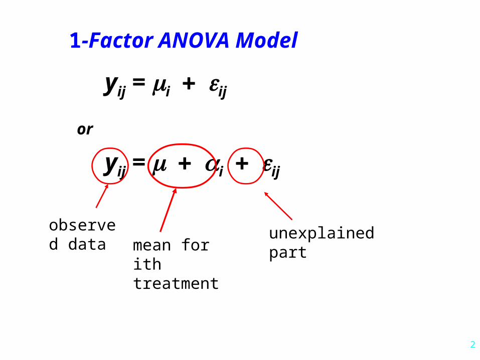
1-Factor ANOVA Model
yij = iij
yij = iij
or
unexplained partmean for ith treatment
observed data
3
0 1 2:
:
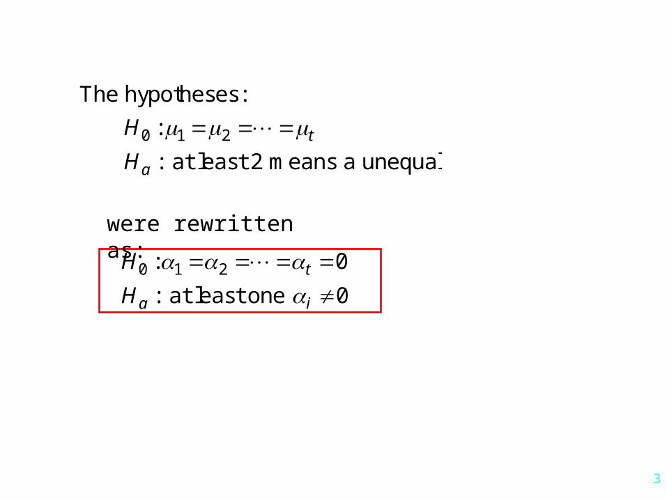
The hypotheses:
at least 2 means a unequalt
a
H
H
0 1 2: 0
: 0
at least one t
a i
H
H
were rewritten as:

4
2 2 2.. . .. .
1 1 1 1 1
( ) ( ) ( )t n t t n
ij i ij ii j i i j
y y n y y y y
TSS SSB SSW Notation:
In words:
TSS(total SS) = total sample variability among yij values
SSB(SS “between”) = variability explained by differences in group means
SSW(SS “within”) = unexplained variability (within groups)

5
Analysis of Variance TableAnalysis of Variance TableAnalysis of Variance TableAnalysis of Variance Table
Note: unequal sample sizes allowed
2
0 2( 1, )B
TW
sH F F t n t
s We reject at significance level if
6
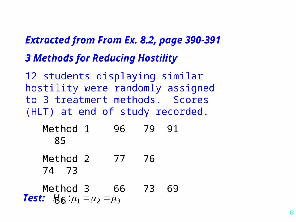
Extracted from From Ex. 8.2, page 390-391
3 Methods for Reducing Hostility
12 students displaying similar hostility were randomly assigned to 3 treatment methods. Scores (HLT) at end of study recorded.
Method 1 96 79 91 85
Method 2 77 76 74 73
Method 3 66 73 69 66
Test: 0 1 2 3:H
7
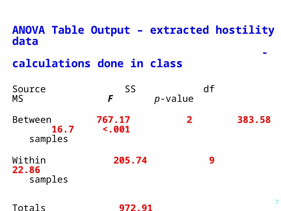
ANOVA Table Output – extracted hostility data - calculations done in class
Source SS df MS F p-value
Between 767.17 2 383.58 16.7 <.001 samples
Within 205.74 9 22.86 samples
Totals 972.91

Protected LSD: Preceded by an F-test for overall significance.
1 2
1 2
22
1 2
1 1( )α/ W
y y
y y
t sn n
and are significantly different if
| | LSD
where
LSD = +
and within (error) df
Unprotected: Not preceded by an F-test (like individual t-tests).
Only use the LSD if F is significant.
Fisher’s Least Significant Fisher’s Least Significant Difference (LSD)Difference (LSD)
X

9
Hostility Data - Completely Randomized Design The GLM Procedure t Tests (LSD) for score
NOTE: This test controls the Type I comparisonwise error rate, not the experimentwise error rate. Alpha 0.05 Error Degrees of Freedom 9 Error Mean Square 22.86111 Critical Value of t 2.26216 Least Significant Difference 7.6482 Means with the same letter are not significantly different.
t Grouping Mean N method
A 87.750 4 1 B 75.000 4 2 B B 68.500 4 3
10
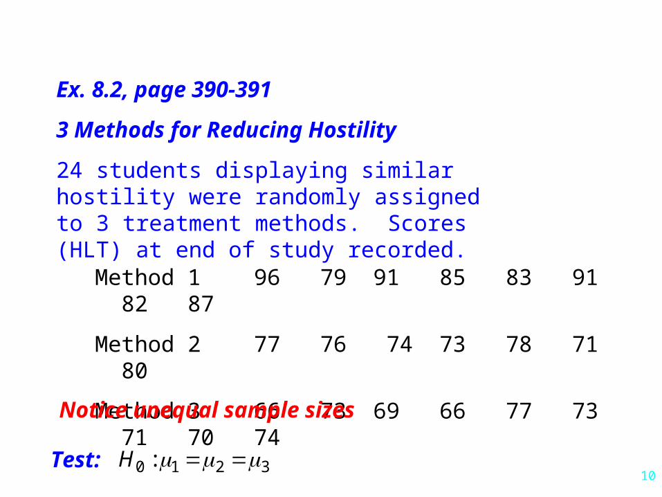
Ex. 8.2, page 390-391
3 Methods for Reducing Hostility
24 students displaying similar hostility were randomly assigned to 3 treatment methods. Scores (HLT) at end of study recorded.
Method 1 96 79 91 85 83 91 82 87
Method 2 77 76 74 73 78 71 80
Method 3 66 73 69 66 77 73 71 70 74
Test: 0 1 2 3:H
Notice unequal sample sizes
11
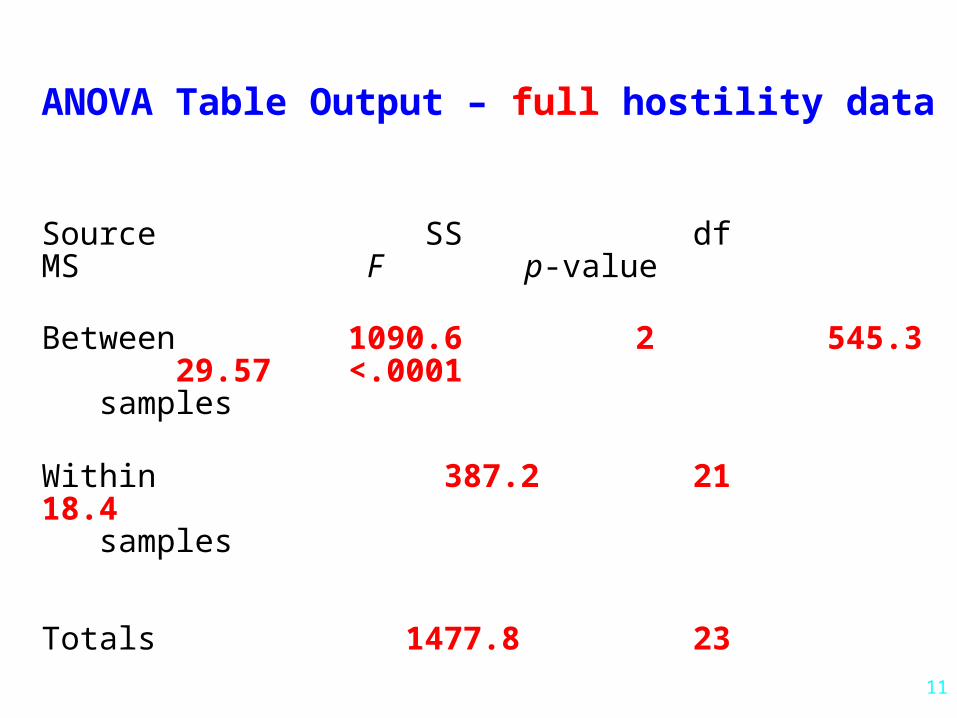
ANOVA Table Output – full hostility data
Source SS df MS F p-value
Between 1090.6 2 545.3 29.57 <.0001 samples
Within 387.2 21 18.4 samples
Totals 1477.8 23
12
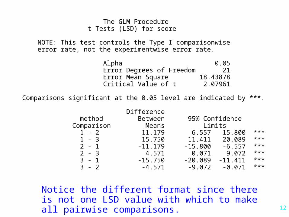
The GLM Procedure t Tests (LSD) for score
NOTE: This test controls the Type I comparisonwise error rate, not the experimentwise error rate. Alpha 0.05 Error Degrees of Freedom 21 Error Mean Square 18.43878 Critical Value of t 2.07961 Comparisons significant at the 0.05 level are indicated by ***.
Difference method Between 95% Confidence Comparison Means Limits 1 - 2 11.179 6.557 15.800 *** 1 - 3 15.750 11.411 20.089 *** 2 - 1 -11.179 -15.800 -6.557 *** 2 - 3 4.571 0.071 9.072 *** 3 - 1 -15.750 -20.089 -11.411 *** 3 - 2 -4.571 -9.072 -0.071 ***
Notice the different format since there is not one LSD value with which to make all pairwise comparisons.

13
Duncan's Multiple Range Test for score
NOTE: This test controls the Type I comparisonwise error rate, not the experimentwise error rate.
Alpha 0.05 Error Degrees of Freedom 21 Error Mean Square 18.43878 Harmonic Mean of Cell Sizes 7.91623
NOTE: Cell sizes are not equal.
Number of Means 2 3 Critical Range 4.489 4.712
Means with the same letter are not significantly different.
Duncan Grouping Mean N method
A 86.750 8 1
B 75.571 7 2
C 71.000 9 3
Note: Duncan’s test (another multiple comparison test) avoids the issue of different sample sizes by using the harmonic mean of the ni’s.
14
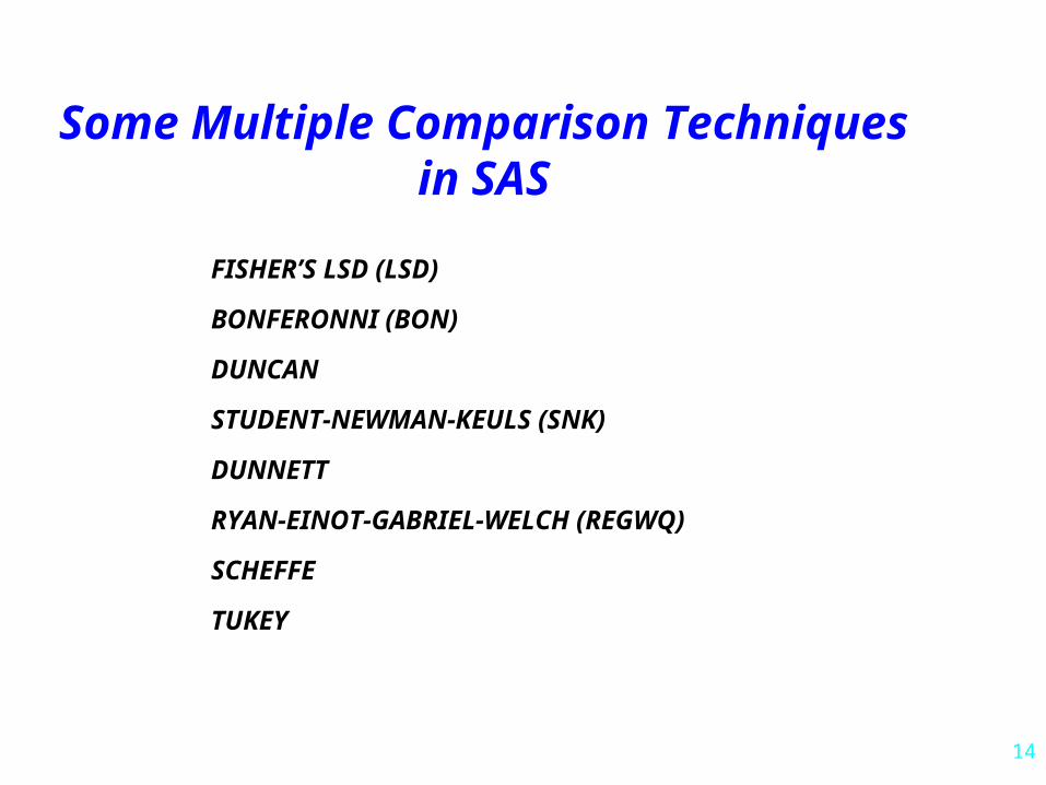
Some Multiple Comparison Techniquesin SAS
FISHER’S LSD (LSD)
BONFERONNI (BON) DUNCAN
STUDENT-NEWMAN-KEULS (SNK)
DUNNETT RYAN-EINOT-GABRIEL-WELCH (REGWQ) SCHEFFE TUKEY
15
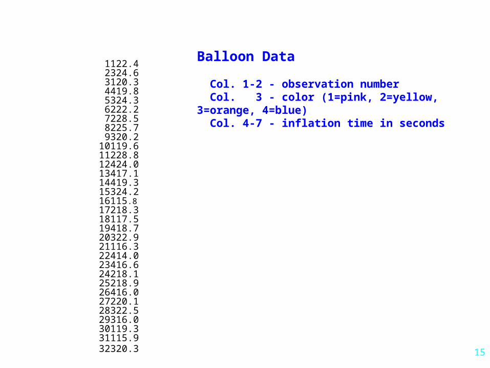
1122.4 2324.6 3120.3 4419.8 5324.3 6222.2 7228.5 8225.7 9320.210119.611228.812424.013417.114419.315324.216115.817218.318117.519418.720322.921116.322414.023416.624218.125218.926416.027220.128322.529316.030119.331115.932320.3
Balloon Data Col. 1-2 - observation number Col. 3 - color (1=pink, 2=yellow, 3=orange, 4=blue) Col. 4-7 - inflation time in seconds

16
1122.4 2324.6 3120.3 4419.8 5324.3 6222.2 7228.5 8225.7 9320.210119.611228.812424.013417.114419.315324.216115.817218.318117.519418.720322.921116.322414.023416.624218.125218.926416.027220.128322.529316.030119.331115.932320.3
Balloon Data Col. 1-2 - observation number Col. 3 - color (1=pink, 2=yellow, 3=orange, 4=blue) Col. 4-7 - inflation time in seconds

17
ANOVA --- Balloon Data General Linear Models Procedure Dependent Variable: TIME Sum of MeanSource DF Squares Square F Value Pr > F Model 3 126.15125000 42.05041667 3.85 0.0200 Error 28 305.64750000 10.91598214 Corrected Total 31 431.79875000 R-Square C.V. Root MSE TIME Mean 0.292153 16.31069 3.3039343 20.256250 MeanSource DF Type I SS Square F Value Pr > F Color 3 126.15125000 42.05041667 3.85 0.0200
18
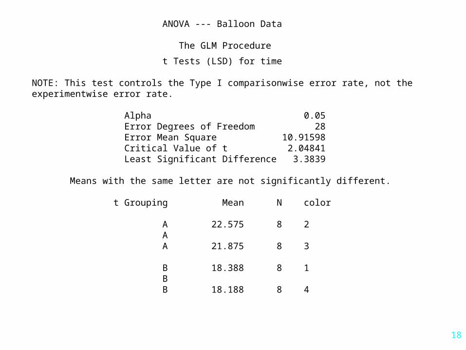
ANOVA --- Balloon Data
The GLM Procedure
t Tests (LSD) for time NOTE: This test controls the Type I comparisonwise error rate, not the experimentwise error rate. Alpha 0.05 Error Degrees of Freedom 28 Error Mean Square 10.91598 Critical Value of t 2.04841 Least Significant Difference 3.3839
Means with the same letter are not significantly different.
t Grouping Mean N color
A 22.575 8 2 A A 21.875 8 3 B 18.388 8 1 B B 18.188 8 4
19
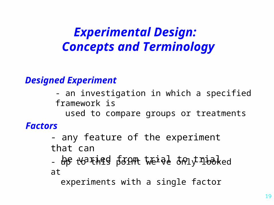
Experimental Design: Concepts and Terminology
Designed Experiment- an investigation in which a specified framework is used to compare groups or treatments
Factors
- up to this point we’ve only looked at experiments with a single factor
- any feature of the experiment that can be varied from trial to trial
20
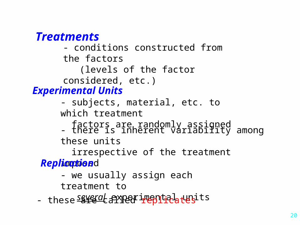
Experimental Units- subjects, material, etc. to which treatment factors are randomly assigned
- there is inherent variability among these units irrespective of the treatment imposed
Replication- we usually assign each treatment to several experimental units
- these are called replicates
- conditions constructed from the factors (levels of the factor considered, etc.)
Treatments
21
Examples:
Car Data
Hostility Data
Balloon Data
1. factor
2. treatments
3. experimental units
4. replicates
22
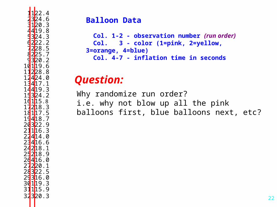
1122.4 2324.6 3120.3 4419.8 5324.3 6222.2 7228.5 8225.7 9320.210119.611228.812424.013417.114419.315324.216115.817218.318117.519418.720322.921116.322414.023416.624218.125218.926416.027220.128322.529316.030119.331115.932320.3
Balloon Data Col. 1-2 - observation number (run order) Col. 3 - color (1=pink, 2=yellow, 3=orange, 4=blue) Col. 4-7 - inflation time in seconds
Why randomize run order? i.e. why not blow up all the pink balloons first, blue balloons next, etc?
Question:
23
t i me
14
15
16
17
18
19
20
21
22
23
24
25
26
27
28
29
i d
0 10 20 30 40
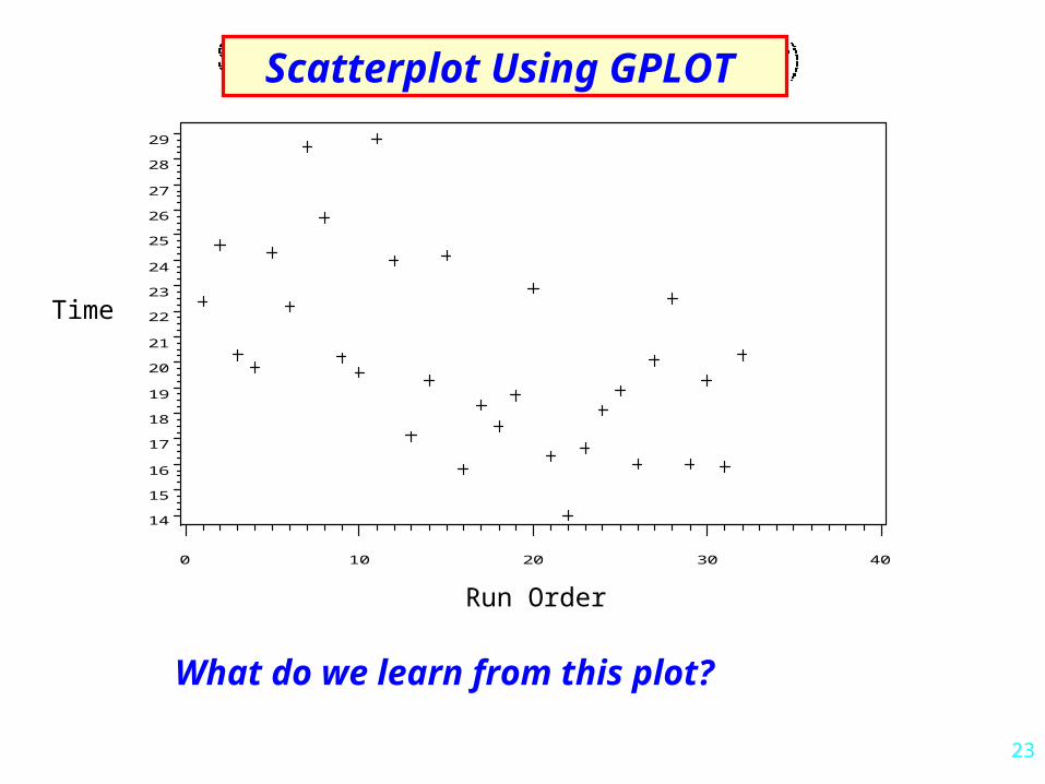
Scatterplot Using GPLOT
What do we learn from this plot?
Run Order
Time
24
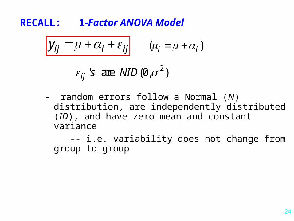
RECALL: 1-Factor ANOVA Model
2 ' are (0, )ij s NID
- random errors follow a Normal (N) distribution, are independently distributed (ID), and have zero mean and constant variance
( )i i ij i ijy
-- i.e. variability does not change from group to group

25
Model Assumptions:
Checking Validity of Assumptions
1. F-test similar to 2-sample case - Hartley’s test (p.366 text) - not recommended
2. Graphical - side-by-side box plots
- equal variances- normality
Equal Variances

26
Graphical Assessment of Equal Variance Assumption
27
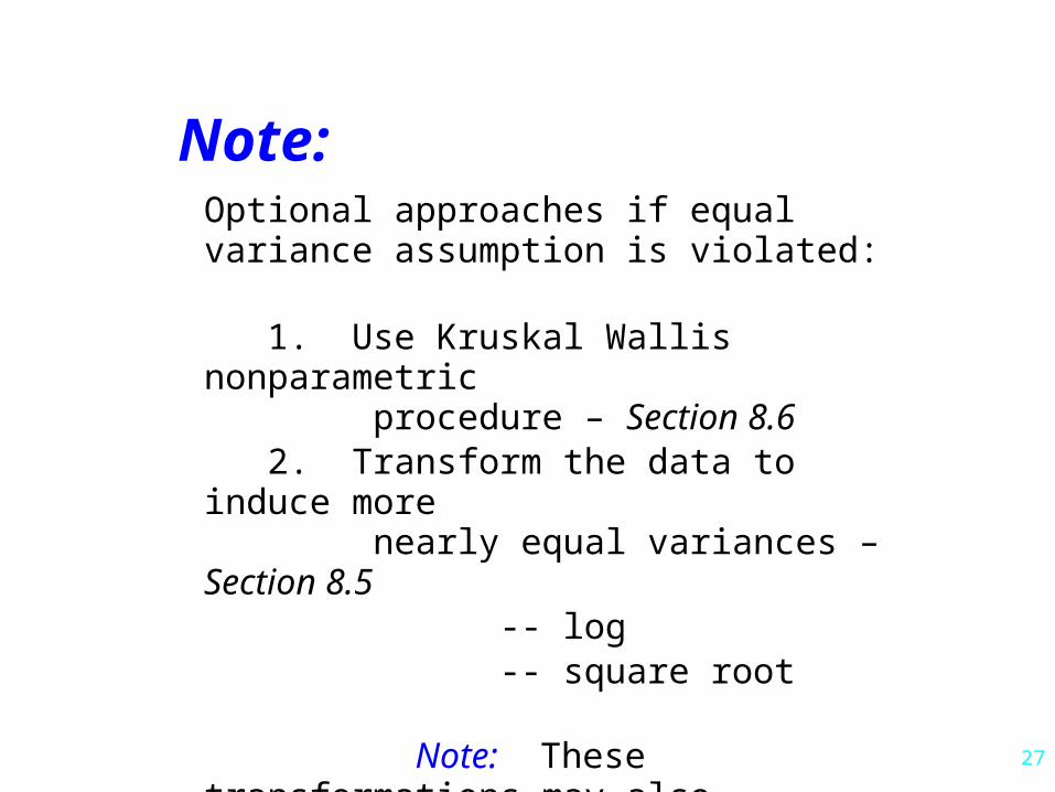
Note:Optional approaches if equal variance assumption is violated:
1. Use Kruskal Wallis nonparametric procedure – Section 8.6 2. Transform the data to induce more nearly equal variances – Section 8.5 -- log -- square root
Note: These transformations may also help induce normality
28
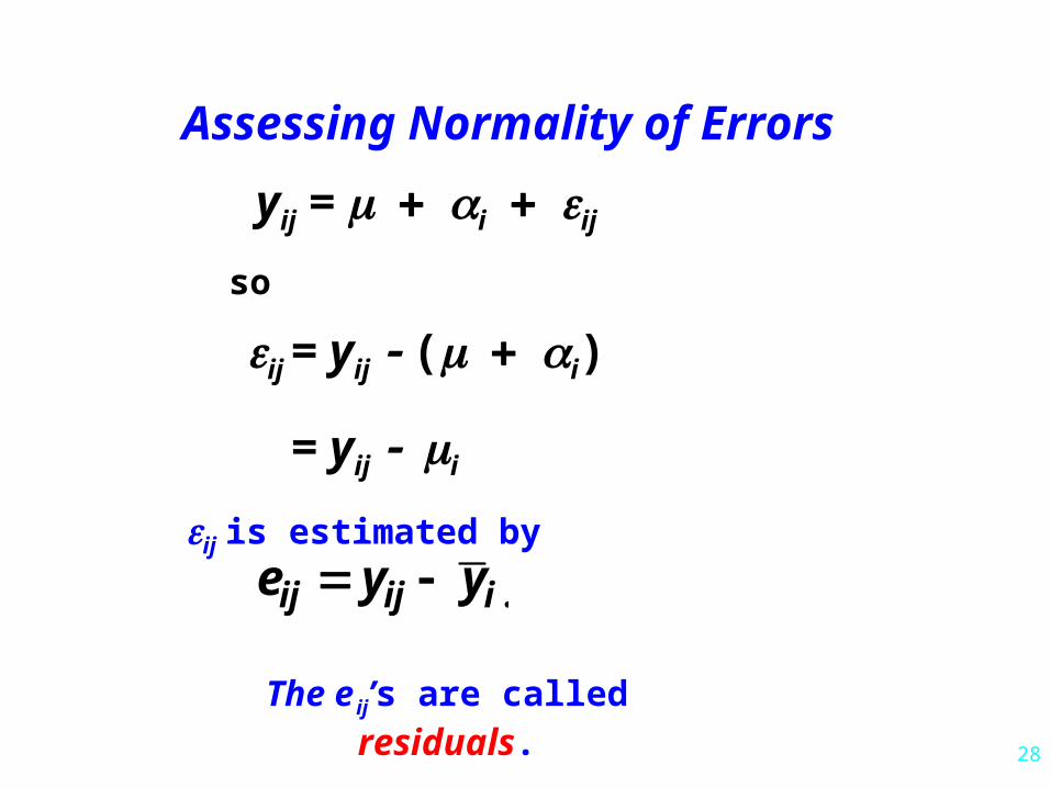
yij = iij
Assessing Normality of Errors
ij = yij (i)so
ij is estimated by
.ij ij ie y y
= yij i
The e ij’s are called residuals.
29
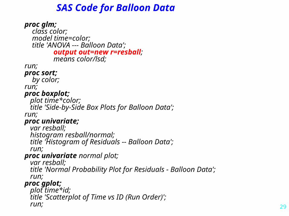
proc glm; class color; model time=color; title 'ANOVA --- Balloon Data';
output out=new r=resball;means color/lsd;
run;proc sort; by color;run;proc boxplot; plot time*color; title 'Side-by-Side Box Plots for Balloon Data';run;proc univariate; var resball; histogram resball/normal; title 'Histogram of Residuals -- Balloon Data'; run;proc univariate normal plot; var resball; title 'Normal Probability Plot for Residuals - Balloon Data'; run;proc gplot; plot time*id; title 'Scatterplot of Time vs ID (Run Order)'; run;
SAS Code for Balloon Data

30
Normal Probability Plot 6.5+ +*+ | * *+++ | *+++ | +*+ | *** | **** 0.5+ ***+ | ++** | ++*** | ***** | +*+ | *+*+* -5.5+ * ++++ +----+----+----+----+----+----+----+----+----+----+
-2 -1 0 +1 +2
.ij ij ie y y Graphical Assessment of Normality of Residuals
- 6 - 3 0 3 6
0
5
10
15
20
25
30
35
40
Percent
r esbal l
31
Caution: Chapter 15 introduces some new notation - i.e. changes notation already defined
32
2 2 2.. . .. .
1 1 1 1 1
( ) ( ) ( )t n t t n
ij i ij ii j i i j
y y n y y y y
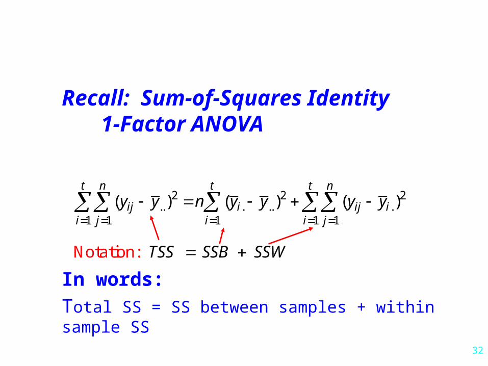
Recall: Sum-of-Squares Identity 1-Factor ANOVA
TSS SSB SSW Notation:
In words:
Total SS = SS between samples + within sample SS
33
2 2 2.. . .. .
1 1 1 1 1
( ) ( ) ( )t n t t n
ij i ij ii j i i j
y y n y y y y
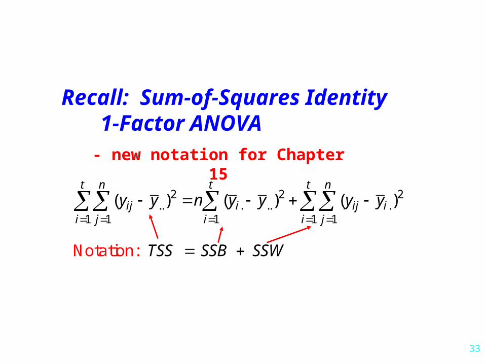
Recall: Sum-of-Squares Identity 1-Factor ANOVA
TSS SSB SSW Notation:
- new notation for Chapter 15

34
2 2 2.. . .. .
1 1 1 1 1
( ) ( ) ( )t n t t n
ij i ij ii j i i j
y y n y y y y
Recall: Sum-of-Squares Identity 1-Factor ANOVA
TSS S SSWST Notation:
- new notation for Chapter 15

35
2 2 2.. . .. .
1 1 1 1 1
( ) ( ) ( )t n t t n
ij i ij ii j i i j
y y n y y y y
Recall: Sum-of-Squares Identity 1-Factor ANOVA
TSS SST SSE Notation:
- new notation for Chapter 15
In words:
Total SS = SS for “treatments” + SS for “error”
36
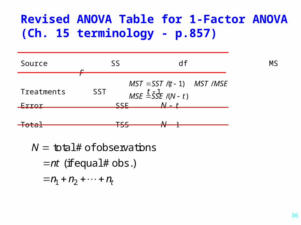
Revised ANOVA Table for 1-Factor ANOVA(Ch. 15 terminology - p.857)
Source SS df MS F
Treatments SST t 1
Error SSE N t Total TSS N
/( 1)MST SST t
/( )MSE SSE N t
/MST MSE
1 2 t
N
nt
n n n
total # of observations
(if equal # obs.)

37
Recall 1-factor ANOVA (CRD) Model for Gasoline Octane Data
yij = iij
yij = iij
or
unexplained partmean for ith gasoline
observed octane
-- car-to-car differences-- temperature-- etc.
38
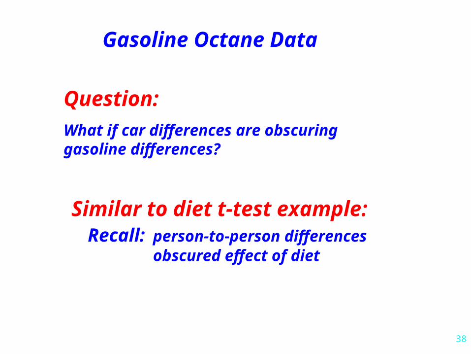
Gasoline Octane Data
Question:
What if car differences are obscuring gasoline differences?
Similar to diet t-test example: Recall: person-to-person differences obscured effect of diet
39
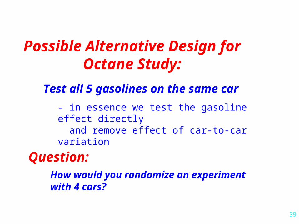
Possible Alternative Design for Octane Study:
Test all 5 gasolines on the same car
- in essence we test the gasoline effect directly and remove effect of car-to-car variation
Question:How would you randomize an experiment with 4 cars?
40
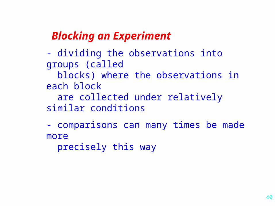
Blocking an Experiment
- dividing the observations into groups (called blocks) where the observations in each block are collected under relatively similar conditions
- comparisons can many times be made more precisely this way
41
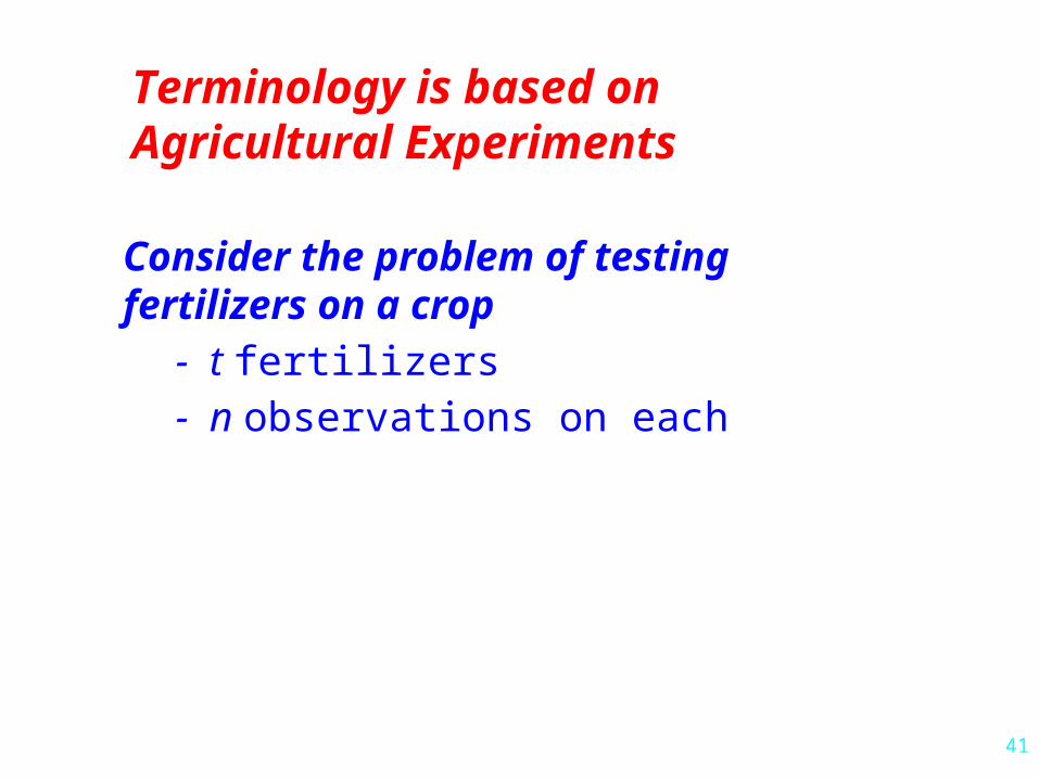
Terminology is based on Agricultural Experiments
Consider the problem of testingfertilizers on a crop - t fertilizers - n observations on each
42
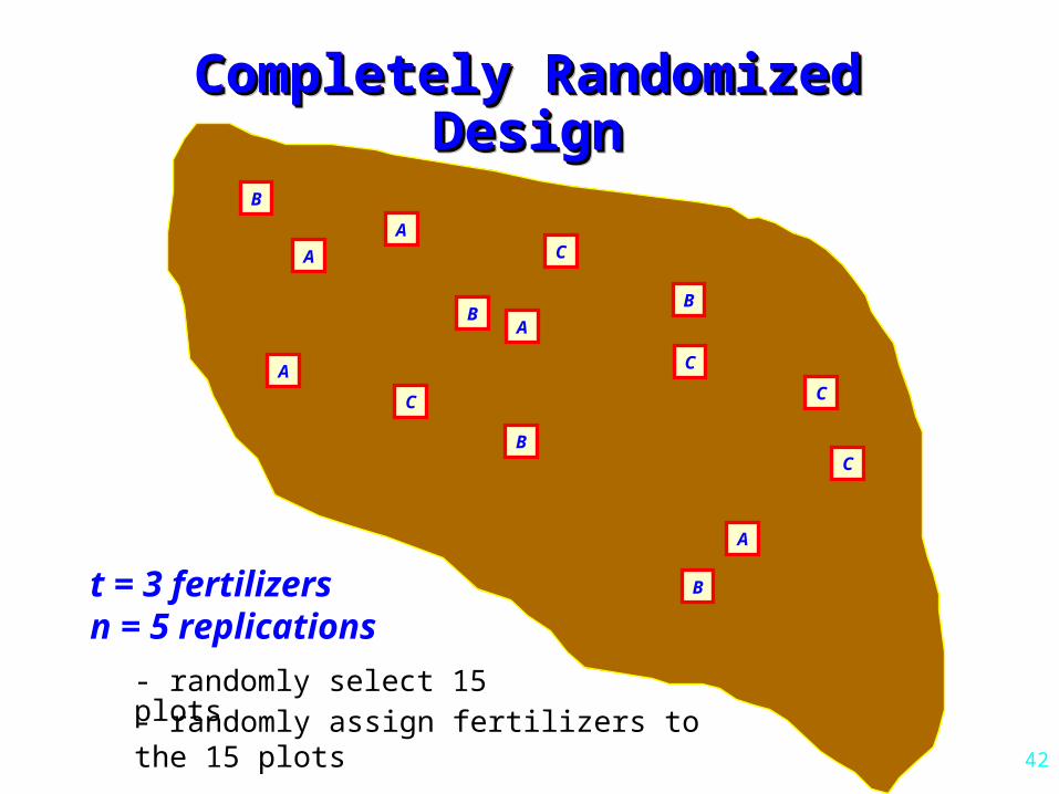
Completely Randomized DesignCompletely Randomized DesignCompletely Randomized DesignCompletely Randomized Design
A
A
BB
C
C
B
A
C
C
B
A
A
B
C
t = 3 fertilizersn = 5 replications
- randomly select 15 plots- randomly assign fertilizers to the 15 plots

43
Randomized Complete Block Randomized Complete Block StrategyStrategy
Randomized Complete Block Randomized Complete Block StrategyStrategy
B | A | C
A | C | B
C | A | B
A | B | C C | B | A
t = 3 fertilizers
- select 5 “blocks”- randomly assign the 3 treatments to each block
Note: The 3 “plots” within each block are similar - similar soil type, sun, water, etc
44
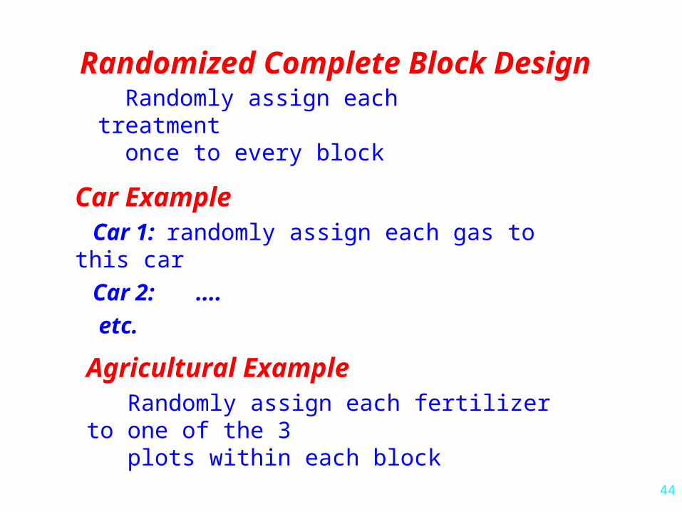
Randomized Complete Block Design Randomly assign each treatment once to every block
Car Example Car 1: randomly assign each gas to this car
Car 2: ....
etc.
Agricultural Example Randomly assign each fertilizer to one of the 3 plots within each block
45
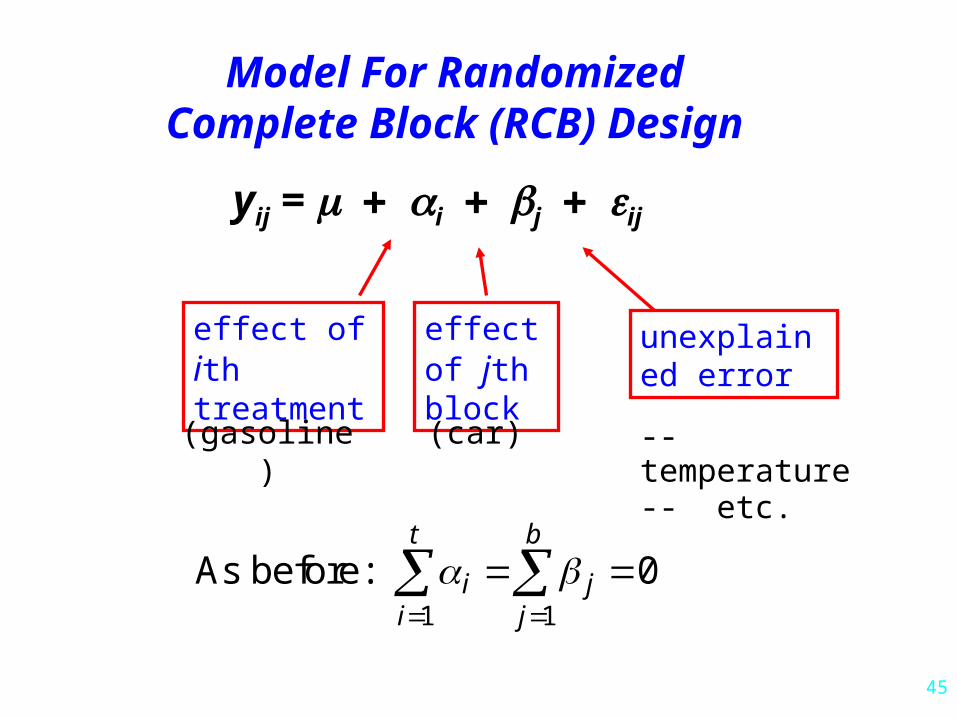
yij = ijij
Model For Randomized Complete Block (RCB) Design
effect of ith treatment
effect of jth block
unexplained error
(car)(gasoline)
1 1
0t b
i ji j
As before:
-- temperature-- etc.
46
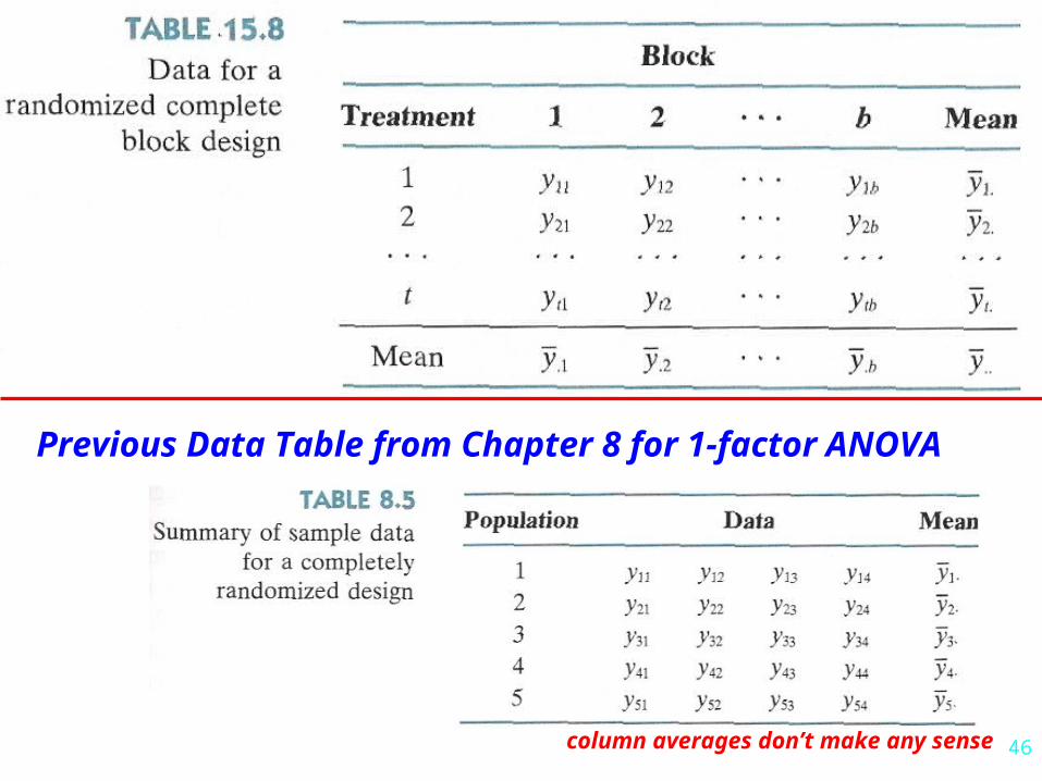
Previous Data Table from Chapter 8 for 1-factor ANOVA
column averages don’t make any sense
47
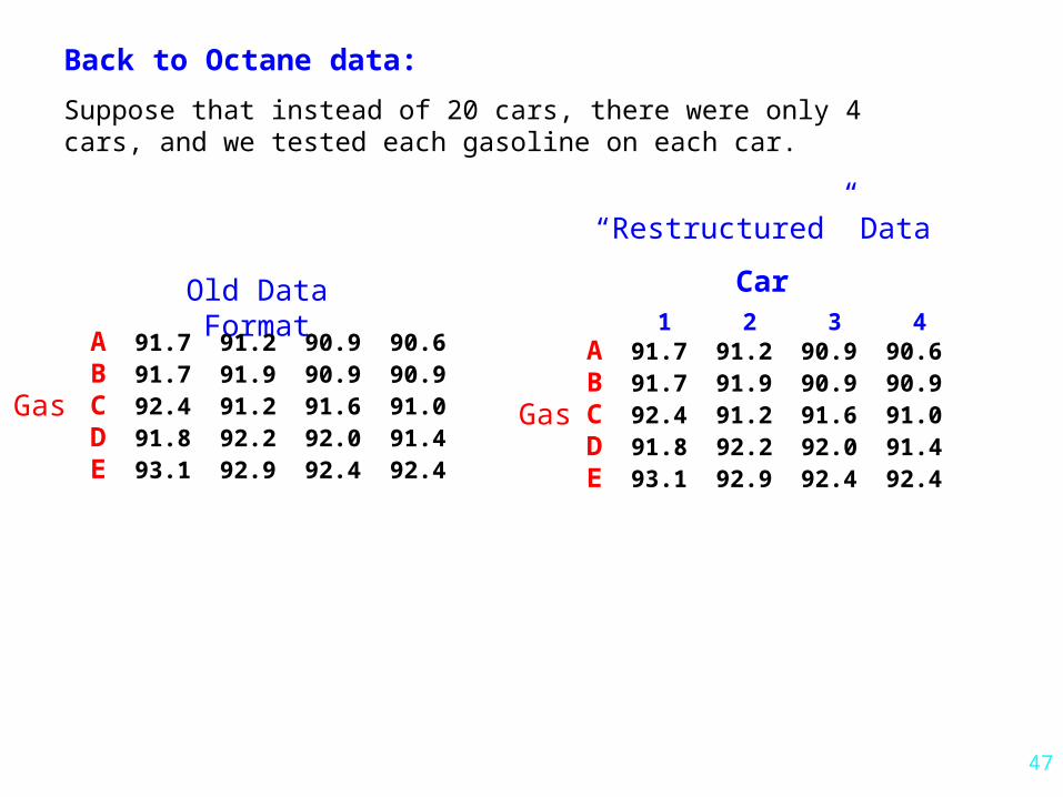
Back to Octane data:
Suppose that instead of 20 cars, there were only 4 cars, and we tested each gasoline on each car.
“Restructured” Data
A 91.7 91.2 90.9 90.6B 91.7 91.9 90.9 90.9C 92.4 91.2 91.6 91.0D 91.8 92.2 92.0 91.4E 93.1 92.9 92.4 92.4
Old Data Format1 2 3 4
Car
Gas
A 91.7 91.2 90.9 90.6B 91.7 91.9 90.9 90.9C 92.4 91.2 91.6 91.0D 91.8 92.2 92.0 91.4E 93.1 92.9 92.4 92.4
Gas
48
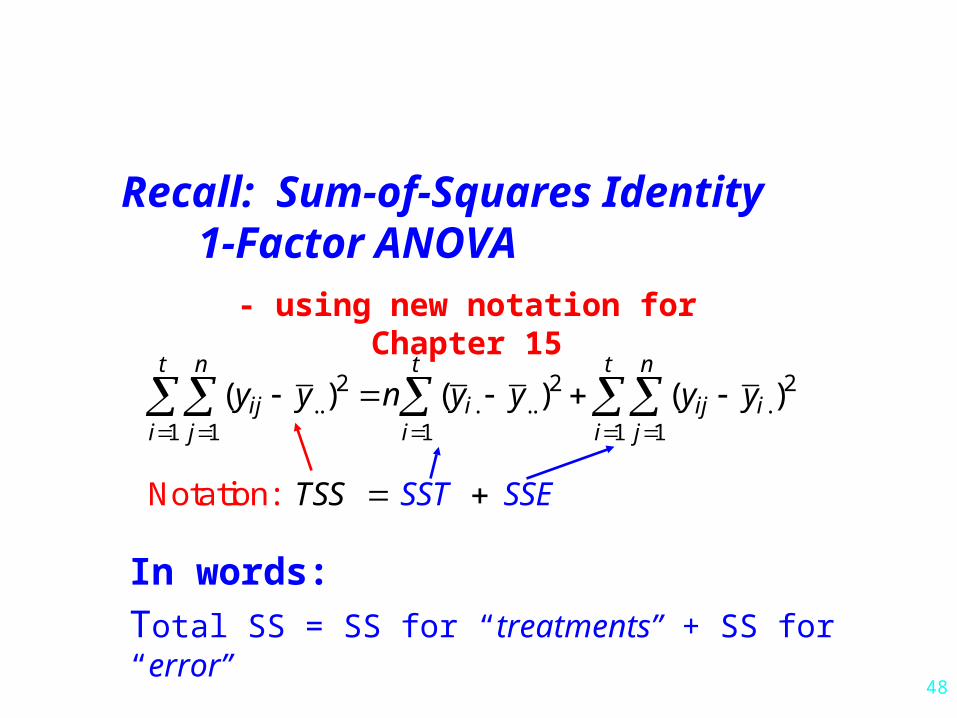
2 2 2.. . .. .
1 1 1 1 1
( ) ( ) ( )t n t t n
ij i ij ii j i i j
y y n y y y y
Recall: Sum-of-Squares Identity 1-Factor ANOVA
TSS SST SSE Notation:
- using new notation for Chapter 15
In words:
Total SS = SS for “treatments” + SS for “error”
49
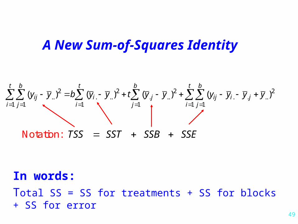
2 2 2 2.. . .. . .. . . ..
1 1 1 1 1 1
( ) ( ) ( ) ( )t b t b t b
ij i j ij i ji j i j i j
y y b y y t y y y y y y
A New Sum-of-Squares Identity
TSS SST SSB SSE Not atio n:
In words:
Total SS = SS for treatments + SS for blocks + SS for error
50
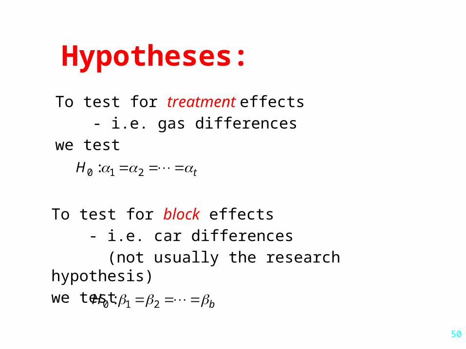
Hypotheses:
To test for treatment effects - i.e. gas differenceswe test
0 1 2: tH
To test for block effects - i.e. car differences (not usually the research hypothesis)we test
0 1 2: bH
51
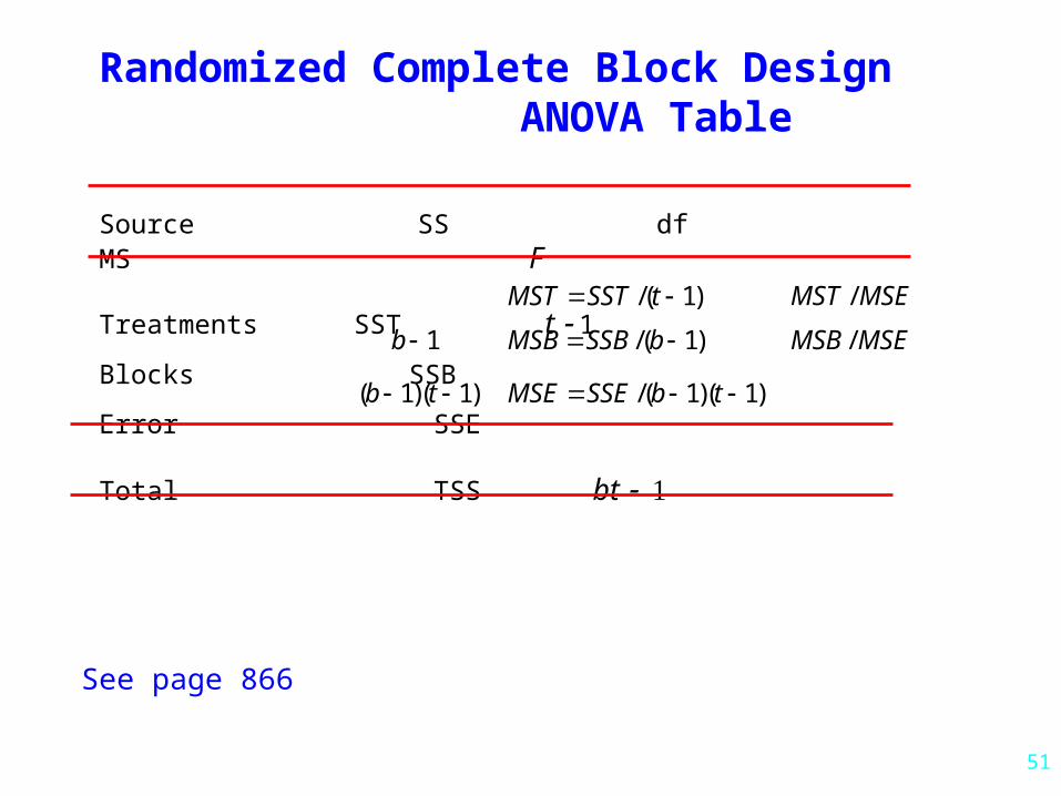
Randomized Complete Block Design ANOVA Table
Source SS df MS F
Treatments SST t 1
Blocks SSB
Error SSE Total TSS bt
/( 1)MST SST t
/( 1)( 1)MSE SSE b t
/MST MSE
See page 866
( 1)( 1)b t
1b /( 1)MSB SSB b /MSB MSE

52
0
( 1,( 1)( 1))
H
MSTF F t b t
MSE
We reject at significance level if
0 1 2:
: 0t
a i
H
H
at least one
Test for Treatment Effects
Note:2MSE estimates
2 2
1
1
1
t
ii
MSTt
estimates
1F - if no treatment effects, we expect ; 1F - if treatment effects, we expect

53
0
( 1,( 1)( 1))
H
MSBF F b b t
MSE
We reject at significance level if
Test for Block Effects
0 1 2:
: 0b
a j
H
H
at least one
54
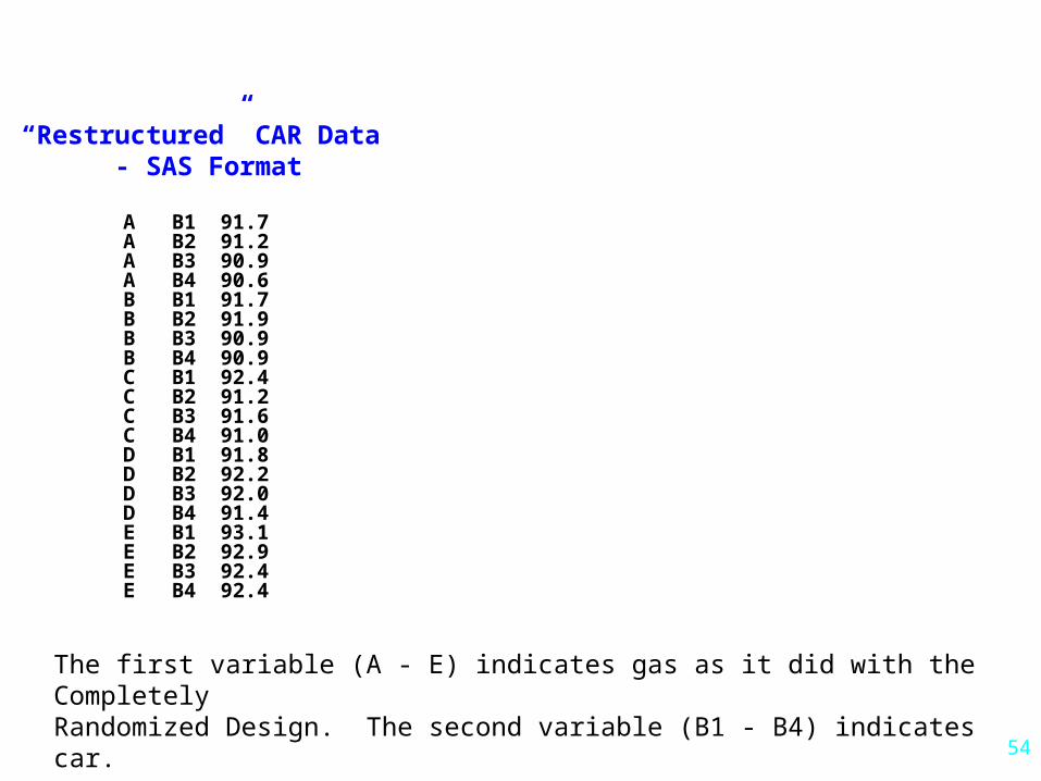
The first variable (A - E) indicates gas as it did with the CompletelyRandomized Design. The second variable (B1 - B4) indicates car.
A B1 91.7A B2 91.2A B3 90.9A B4 90.6B B1 91.7B B2 91.9B B3 90.9B B4 90.9C B1 92.4C B2 91.2C B3 91.6C B4 91.0D B1 91.8D B2 92.2D B3 92.0D B4 91.4E B1 93.1E B2 92.9E B3 92.4E B4 92.4
“Restructured” CAR Data - SAS Format

55
SAS file - Randomized Complete Block Design for CAR Data
INPUT gas$ block$ octane;PROC GLM; CLASS gas block; MODEL octane=gas block; TITLE 'Gasoline Example -Randomized Complete Block Design'; MEANS gas/LSD;RUN;
56
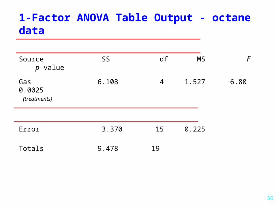
1-Factor ANOVA Table Output - octane data
Source SS df MS F p-value
Gas 6.108 4 1.527 6.80 0.0025 (treatments)
Error 3.370 15 0.225
Totals 9.478 19
57
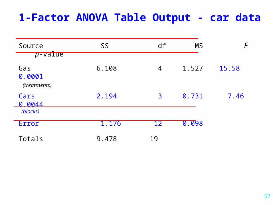
1-Factor ANOVA Table Output - car data
Source SS df MS F p-value
Gas 6.108 4 1.527 15.58 0.0001 (treatments)
Cars 2.194 3 0.731 7.46 0.0044 (blocks)
Error 1.176 12 0.098
Totals 9.478 19
58
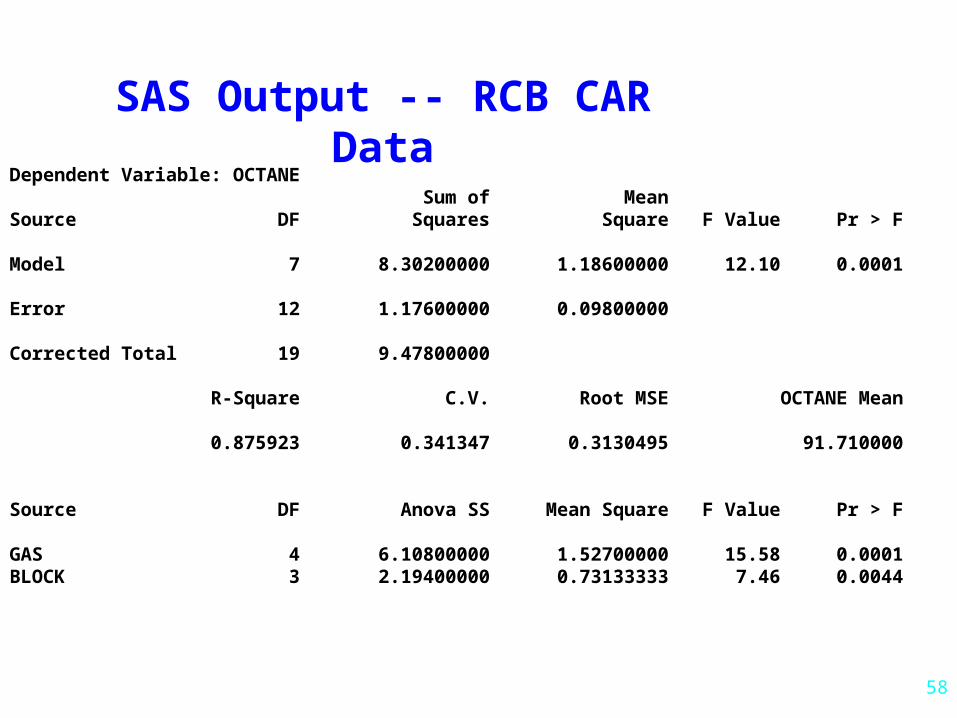
Dependent Variable: OCTANE Sum of MeanSource DF Squares Square F Value Pr > F Model 7 8.30200000 1.18600000 12.10 0.0001 Error 12 1.17600000 0.09800000 Corrected Total 19 9.47800000 R-Square C.V. Root MSE OCTANE Mean 0.875923 0.341347 0.3130495 91.710000 Source DF Anova SS Mean Square F Value Pr > F GAS 4 6.10800000 1.52700000 15.58 0.0001BLOCK 3 2.19400000 0.73133333 7.46 0.0044
SAS Output -- RCB CAR Data
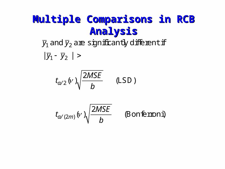
1 2
1 2
y y
y y
and are significantly different if
| |
Multiple Comparisons in RCB AnalysisMultiple Comparisons in RCB Analysis
22
( )α/MSE
tb
(LSD)
(2 )2
( )α/ mMSE
tb
(Bonferroni)
60
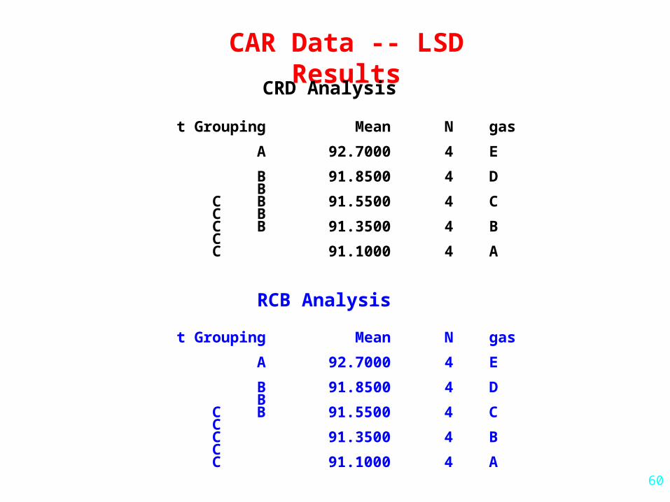
t Grouping Mean N gas A 92.7000 4 E B 91.8500 4 D B C B 91.5500 4 C C B C B 91.3500 4 B C C 91.1000 4 A
t Grouping Mean N gas A 92.7000 4 E B 91.8500 4 D B C B 91.5500 4 C C C 91.3500 4 B C C 91.1000 4 A
CAR Data -- LSD Results
CRD Analysis
RCB Analysis

61
Bon Grouping Mean N gas A 92.7000 4 E A B A 91.8500 4 D B B 91.5500 4 C B B 91.3500 4 B B B 91.1000 4 A
CAR Data -- Bonferroni Results
CRD Analysis
RCB Analysis
Bon Grouping Mean N gas
A 92.7000 4 E
B 91.8500 4 D B B 91.5500 4 C B B 91.3500 4 B B B 91.1000 4 A