1

Effect of Delay and Buffering on Jitter-Free

Streaming over Random VBR Channels

Guanfeng Liang, Student Member, IEEE, and Ben Liang, Senior Member, IEEE

Abstract

We study the optimal streaming of variable bit-rate (VBR) video over a random VBR channel. The

goal of a streaming application is to enable the successful decoding of each video object before its

displaying deadline is violated. Hence, we define the main performance metric of a streaming system

as the probability of un-interrupted video presentation, or jitter-free probability. Previous literature has

described solutions to estimate the jitter-free probability by assuming either independence in the encoded

data process or simplistic channel models. In this work, we present a novel analytical framework, which

requires only some basic statistical information of an arbitrary VBR channel, to bound the probability of

jitter-free playout under the constraint of initial playout delay and receiver buffer size. Both the infinite

and finite buffer cases are considered. This technique is then applied to investigate streaming over a

wireless system modeled by an extended Gilbert channel with ARQ transmission control. Experimental

results with MPEG-4 VBR encoded video demonstrates that the proposed analysis derives close bounds

to the actual system performance. Finally, we show that the proposed analysis provides a theoretical

foundation to quantify the tradeoffs between the initial playout delay, the receiver buffer size, and the

jitter-free probability for a general class of VBR streaming over random VBR channels.

Index Terms

EDICS: 5-STRM; multimedia streaming, performance modeling, playout delay, receiver buffering,

playout interruption

A preliminary version of this paper was presented at the International Conference on Quality of Service in HeterogeneousWired/Wireless Networks (QShine) in 2006. This work was supported in part by a grant from the Natural Sciences andEngineering Research Council of Canada and by Bell Canada through its Bell University Laboratories R&D program. Theauthors are with the Department of Electrical and Computer Engineering, University of Toronto, 10 King’s College Road,Toronto, Ontario, M5S 3G4, Canada. Email:{guanfeng, liang}@comm.utoronto.ca. Tel:+1-416-946-8614. Fax:+1-416-978-4425.

2

Base Station

VBRChannel Receiver

BufferNetwork

BackboneServer

Streaming

bit

s

t

bit

s

t

Mobile Client

Receiver CurvePlayback Curve Playout Curve

t

bit

s

Fig. 1. A typical media streaming system.

I. INTRODUCTION

Mobile devices of the near future are expected to bring ubiquitous access to streaming

multimedia services, such as TV news, music video, and online movies. Streaming multimedia

are likely to become major applications in future mobile systems and may indeed be a key factor

for their success. However, both wired and wireless, but especially wireless, multimedia delivery

face several challenges, such as bandwidth scarcity, random channel variation, and limited storage

capacity [1]. In this work, we focus on the streaming of pre-encoded video to mobile clients,

taking into account these system constraints and limited resources.

A general media streaming system is shown in Figure 1. It consists of a media streaming server,

a transport channel, and a streaming client. The server stores a number of pre-encoded video

objects in the wired backbone network. We consider general variable bit-rate (VBR) encoded

videos with non-linear playback curves [2]. These video objects are accessed by the clients,

through a wire or wireless access network.

In general, the transmission rate of the channel varies over time. Video display interruption may

occur if data are not delivered on time when the transmission rate does not match the encoded

rate. The event of playout interruption is termed jitter. Clearly, jitter reduces the perceived video

quality and is undesirable in video streaming.

To alleviate the detrimental effect of channel and data bit rate variation on jitter-free playout,

3

a common approach is to delay the initial playout of a stream through buffering at the receiver.

The challenges are two-fold. First, both buffer underflow and buffer overflow may occur and

lead to jittering. Hence, a suitable buffer size must be determine. Second, as we are interested

in providing continuous video streaming service, the initial playout delay should be minimized.

In this work, we present an analytical framework to quantify the fundamental tradeoffs between

the initial playout delay, the receiver buffer size, and the jitter-free playout probability, in

order to optimize the streaming of VBR encoded video over a random VBR channel. Our

main contributions are three-fold. First, we derive the upper and lower bounds of jitter-free

probability given the initial playout delay and receiver buffer size, for both infinite buffers

and finite buffers. The proposed analysis technique provides a means to maximize the jitter-

free probability for a general class of VBR multimedia streaming over random VBR channels.

Second, we apply the proposed analytical framework toward optimal streaming over a general

wireless network. Numerical analysis results are obtained for wireless systems modelled by an

extended Gilbert-Elliot channel with ARQ transmission control. Third, experiments using sample

MPEG-4 video traces are carried out to validate the proposed analysis and provide new insights

into the optimal balancing of the initial playout delay and the receiver buffer size for optimal

multimedia streaming.

The rest of this paper is organized as follows. We discuss related works in Section II. In

Section III, an analytical framework is presented to bound the jitter probability under constraints

of initial delay and receiver buffer size. This framework is applied to a wireless system to

derive QoS bounds in Section IV. Section V provides the numerical and experimental results

and discusses the performance tradeoffs. Conclusions are drawn in Section VI.

4

II. RELATED WORK

One obvious way to avoid jitter is to start displaying the video only after it is fully downloaded.

By doing this, jitter is 100% avoidable, but it also results in the longest initial delay and the

maximal buffer size, which is generally unacceptable, especially for small wireless devices.

In practice, the system buffers a certain portion of video data at the client before displaying

the video, so that transient packet losses and delay do not constantly interrupt the playout of

the stream. Intuitively, the more data is buffered, the lower is the probability of jitter, but the

startup delay induced by buffering increases, too. For this reason, system designers must trade

the reliability of uninterrupted playout against delay and buffer size.

In this context, Sen et al proposed an online smoothing technique for VBR streaming video

in [3] by introducing a few seconds of startup delay and a client buffer to compensate for the

variation of video encoding rate. The authors of [4] used network calculus analysis to derive

an optimal multimedia smooth scheme. However, both schemes require a dedicated smoothing

server or an intermediate smoothing node and only consider a wired network offering guaranteed

bandwidth service. Therefore these schemes are not suitable for error-prone networks such as

wireless streaming systems.

The authors of [5] introduced the concept of having two buffers at the receiver - a delay jitter

buffer and a decoder buffer. The delay jitter buffer is used to compensate for the delay jitter

introduced by the channel and to reduce bit rate variations caused by the VBR behavior of the

channel. Streaming video data is first buffered in the delay jitter buffer and then is emitted into

the decoder buffer at a constant rate R after a initial delay �1. By choosing a suitable �1, the

jittered streaming data is de-jittered by the delay jitter buffer and a virtual CBR channel with

rate R is formed at the input of the decoder buffer. Therefore, traditional hypothetical reference

5

decoders (HRD) such as the video buffer verifier (VBV) for MPEG-2 or the H.263 HRD can

be applied.

In [6], the authors compared the single receiver buffer approach with the aforementioned

separate buffer approach and showed that a single receiver buffer always performs at least as good

as two separate buffers. They then described a method to provide a certain QoS guarantee, where

the initial delay and receiver buffer size are decided according to the upper and lower bounds of

the random receiver curve, R(t), to guarantee a minimum jitter-free probability. However, they

did not give a general means to find such bounds of R(t), and only a simple Bernoulli channel

was considered.

A Markov chain analysis method was introduced in [7] to examine the tradeoff between the

buffer underflow probability and the latency for Adaptive Media Playout (AMP) video streaming.

Applying the two-state Gilbert-Elliott lossy channel model [8], [9], this method represents the

streaming system with a Markov chain whose states are described as a combination of the buffer

state, the channel state and the playout position. Representing underflow event as an absorption

state, this method gives the underflow probability by solving the Markov chain. However, in

order to construct a Markov chain, the transmission times of the data frames are assumed to be

independent and identically distributed (i.i.d.) random variables, which is may not be realistic

for VBR encoded video streaming where the frame sizes are different. Other previous research

studies on jitter reduction include works on rate-distortion optimized video streaming [10], [11],

[12]. They require significant modifications in the streaming server, the streaming client, or both.

In this work, we consider the single receiver buffer setup as in [6] and propose a novel

analytical framework to bound the jitter probability for generic VBR streaming video over random

VBR channels. The proposed framework can be applied to most general systems and only

6

requires basic statistical information about the channel. To the best of our knowledge, this paper

represents the first attempt to analytically quantify the the tradeoffs between initial playout delay,

receiver buffer size, and the jitter free probability for streaming with arbitrary encoding scheme

and arbitrary random channels.

III. STREAMING VIDEO OVER VBR CHANNELS

In this section, we provide an analytical framework to bound the jitter-free probability for

generic VBR streaming over random VBR channels. The application of this analysis to a case

study on wireless network streaming is presented in the next section.

A. System Model

We consider the same video streaming system as in [6]. It consists of a video streaming

server, a generic VBR transport channel with maximum transmission rate bmax, and a streaming

client. Pre-encoded video objects are stored in the server. Each video object is characterized by

a playback curve p(t). The playback curve describes the total amount of data that have to be

received by time t. It is generally assumed that p(t) = 0 for t ≤ 0 and p(t) = p(L) for t ≥ L,

where L is the length of the video in time and p(L) is the size of the video in bits. The playback

curve is assumed to be included in the preamble of the video stream and is available to the

receiver [6].

When a client requests a video object, after setting up a connection, the server starts to stream

video data to the client through the transport channel. The channel is assumed to be error free,

possibly due to an ideal error control mechanism, such as coding or ARQ, but its bit rate may

vary over time. This VBR channel is characterized by a random receiver curve R(t), which

specifies the total amount of data received error-free up to time t at the client side. We also

7

assume R(t) = 0 for t ≤ 0, which is reasonable since no data should be received before

the transmission begins. Clearly, both of p(t) and R(t) are monotonically increasing. This is a

generalization of the CBR channel case in which the receiver curve is linear, i.e., r(t) = Rt·u(t).

As we are interested in providing continuous video streaming service, our objective is to

minimize the initial playout (“startup”) delay � and the corresponding receiver buffer size B,

while maintaining jitter-free playout, for a VBR channel. For jitter-free playout, both buffer

underflow and overflow at the receiver buffer need to be eliminated. To avoid buffer underflow,

the startup delay � has to be chosen such that for any time instant t, at least p(t−�) bits are

available at the decoder, i.e.,

{� ∈ � : ∀t ≤ L, R(t) ≥ p(t −�)}. (1)

Furthermore, to avoid buffer overflow, the buffer size B has to be large enough such that at any

time instant t, all received non-decoded data can be stored in the receiver buffer, i.e.,

{B ∈ � : ∀t ≤ L, R(t) ≤ p(t −�) + B}. (2)

The right-hand side of (1) defines a delayed playback curve, and the right-hand side of (2)

defines a buffer limit curve. Note that, in some situations, jitters can be avoided in the case of

buffer overflow, if the receiver can request retransmission later when there is free space in its

buffer. However, this requires an application-layer mechanism for the client to send a message

to the server requesting a pause/resume in streaming. Such a mechanism may or may not be

available depending on the implementation of the system. In this paper, we treat buffer overflow

and underflow equally following the same assumption used in [6].

If a deterministic receiver curve R(t) and the playback curve p(t) are known before transmis-

8

00

B

time

data

Δ

Playout curveReceiver curveBuffer limit curve

Fig. 2. Playout, receiver, and buffer-limit curves with their associated startup delay � and buffer size B.

sion at the streaming server, the authors of [6] have proven that the minimum startup delay to

avoid buffer underflow should be chosen as

� = maxt

{t − p(−1)(R(t))

}, (3)

where p(−1)(x) � min{t : x ≤ p(t)} is the so called the pseudoinverse function of the

monotonically increasing playback curve p(t). And the corresponding minimum receiver buffer

size to avoid buffer overflow is then chosen as

B = maxt

{R(t) − p(t −�)} (4)

The optimal selection of � and B is illustrated in Figure 2.

However, in general, R(t) is random and not known in advance, either at the transmitter or

at the receiver. In this work, we focus on the problem of optimal streaming over VBR channels

with a random R(t), described in detail next in Section III-B.

9

B. Random Receiver Curve

The assumption that R(t) is known in advance at the transmitter or receiver is obviously not

realistic for most practical systems. To the best of our knowledge, there is no known method to

specify the minimum startup delay without exact knowledge of the receiver curve. However, in

general, users may still be satisfied if the playout jitters do not occur too frequently. Therefore,

it is reasonable to guarantee a certain performance criterion, by specifying the probability that

the transmission of a video is successful without any buffer underflow or buffer overflow, given

the constraint of startup delay and receiver buffer size.

To formalize the problem, let us consider a stationary-increment random process R(t) that

describes the random receiver curve introduced by the random channel. Obviously, each real-

ization of the random process has the same monotonic properties as the deterministic receiver

curve as we defined before. We want to determine the jitter-free probability, denoted by π, that

a realization of R(t) is entirely within the region between the delayed playback curve, p(t−�),

and the buffer limit curve, p(t −�) + B, during the playout period of a video, i.e.,

π � Pr {∀t ≤ L, p(t −�) ≤ R(t) ≤ p(t −�) + B} . (5)

Generally, π is a difficult quantity to compute exactly, even if we know the stochastic properties

of R(t). Next, we will derive a lower bound and an upper bound of π, given some statistical

information of R(t).

C. Infinite Receiver Buffer Case

Let us first look at the case with infinite receiver buffer, i.e., B = ∞ or B is sufficiently large

for any practical purposes such that the buffer never overflows. Since we know that the receiver

10

curve R(t) always has a sloop less then bmax, i.e., R′(t) ≤ bmax for all t. In the best case, the

VBR channel stays at the maximum bit rate bmax throughout the transmission. Without loss of

generality, we fix the origin at the time instant when the client starts playing out the video. Then

the receiver curve in the best case is

Rbest(t) = bmax(t + �min) · u(t + �min) (6)

where u(t) is the unit step function

u(t) =

⎧⎪⎪⎨⎪⎪⎩

0, t < 0

1, t ≥ 0

, (7)

and �min is the minimal achievable startup delay given by (3) with R(t) = bmaxt · u(t), i.e.,

�min = maxt

{t − p−1(bmaxt · u(t))

}. (8)

Note that �min can only be achieved in the best case. It is in fact the minimum supportable

startup delay. By supportable, we mean

Pr {∀t ≤ L, R(t) ≥ p(t) | ∀t ≤ −�, R(t) = 0} > 0. (9)

Therefore, the startup delay should be chosen such that � ≥ �min. The derivation of π then

proceeds in two cases as shown in Figure 3.

Case I. Rbest(L) = p(L)

Let t0 = inf{t : R(t) < Rbest(t)}. If t0 < L, it is easy to see that R(t) < Rbest(t), ∀ t ≥ t0,

11

as shown in Figure 3(a). And therefore at the end of the video, we will have

R(L) < Rbest(L) = p(L). (10)

According to the monotonically increasing property of p(t), jitter is inevitable for this R(t).

Then, it is easy to show that, given a supportable startup delay �, the probability of continuous

playout is

π = Pr{∀t ≤ L, R(t) ≥ p(t)}

= Pr{t0 ≥ L}

= Pr{∀t ≤ L, R(t) ≥ Rbest(t)}

= Pr{R(L) ≥ Rbest(L)}. (11)

Case II. Rbest(L) > p(L)

We define the latest most critical point tc of underflowing as

tc = max {t : Rbest(t) = p(t)} , (12)

and the transmission finishing point tf in the ideal case with minimal startup delay �min as

tf =p(L)

bmax−�min. (13)

Clearly, if t0 ≥ tf , jitter does not occur; if tc ≤ t0 < tf , jitter may not occur with positive

probability; and if t0 < tc, jitter occurs. An example when t0 < tc is shown in Figure 3(b).

12

Hence we can derive a lower bound on π as follows:

π = Pr{t0 ≥ tf} + Pr{∀t ≤ L, R(t) ≥ p(t) and tc ≤ t0 < tf}

≥Pr{t0 ≥ tf}

= Pr{∀ t ≤ tf , R(t) ≥ Rbest(t)}

= Pr{R(tf ) ≥ p(L)} Δ= πl. (14)

Moreover, noticing that ddt

p(t) < bmax for some t ∈ [tc, L], it is possible that even if a

jitter incident occurs, R(t) may increase faster than p(t) and, at the end of the video, achieve

R(L) ≥ p(L). Hence π is upper bounded by the probability of receiving no less than p(L) bits

by the end of the video, i.e.,

π ≤ πuΔ= Pr{R(L) ≥ p(L)}. (15)

In summary, when a supportable startup delay � ≥ �min is chosen, the jitter free probability

of a given playback curve p(t) is bounded by πl and πu according to (14) and (15), respectively.

Both bounds are achieved iff Rbest(L) = p(L).

Moreover, the difference between the upper bound and lower bound πu − πl represents the

tightness of the bounds. However, in most cases, the exactly analysis of this gap requires precise

statistic of the channel and video, and it is in general mathematically intractable. From the

analysis above, we can conclude that the value of this gap depends on the characteristic of the

VBR channel’s stochastic behavior, and the shape of the video’s playout curve as well. Generally

speaking, the closer the critical point tc is to the end of the video, or the closer Rbest(t) is to p(t)

by the end of video, the tighter the bounds will be, i.e., small values of L−tc or Rbest(L)−p(L)

13

0 L0

p(L)

time

data

−Δ −Δmin t

0

p(t)R

best(t)

R(t)

(a) Case I: Rbest(L) = p(L)

0 L0

p(L)

time

data

−Δ −Δmin t

0tc

tf

p(t)R

best(t)

R(t)

(b) Case II: Rbest(L) > p(L), t0 < tc

Fig. 3. Examples of infinity receiver buffer.

will result in a small value of πu − πl.

D. Finite Receiver Buffer Case

When the receiver buffer is not large enough, overflow may occur. We will derive bounds on

the probability that neither underflow nor overflow occurs.

14

0 L0

B

p(L)

p(L)+B

time

data

−Δ −ΔB

−Δmin t

Bt1

p(t)R

best(t)

R(t)p(t)+BR

B(t)

bmax

(t+Δ)

Fig. 4. An example of finite receiver buffer.

Let tB denote the first most critical point of overflowing:

tB = min{arg maxt

{Rbest(t) − p(t)}}. (16)

Obviously, if the buffer size is a design parameter, then B should be chosen such that

B ≥ Rbest(tB) − p(tB) � Bmin. (17)

Otherwise jitter (either overflow or underflow) is inevitable. Let

RB(t) = bmax(t + �B), (18)

where

�B = mint

{p(t) + B

bmax− t

}, (19)

is the highest supporting line of the buffer limit curve p(t) + B with slope bmax. An example

of this finite buffer case is shown in Figure 4.

15

We first consider a lower bound of π. It can be shown that

π = Pr{no underflow and no overflow}

= Pr{∀ t ≤ L, p(t) ≤ R(t) ≤ p(t) + B}

= Pr{∀t ≤ L, R(t) ≥ p(t)}

−Pr{∃t ≤ L, R(t) > p(t) + B and ∀t ≤ L, R(t) ≥ p(t)}

≥Pr{∀t ≤ L, R(t) ≥ p(t)} − Pr{∃t ≤ L, R(t) > p(t) + B}

≥Pr{R(tf ) ≥ p(L)} − Pr{∃t ≤ L, R(t) > p(t) + B}. (20)

Then, let

t1 = min{t : bmax(t + �) = p(t) + B} (21)

be the first possible point of overflowing when startup delay is �. It is easy to see that if

R(t1) ≤ RB(t1), overflow does not happen, i.e.

Pr{R(t1) ≤ RB(t1)} ≤ Pr{∀t ≤ L, R(t) ≤ p(t) + B}. (22)

Hence, we have

Pr{R(t1) > RB(t1)} ≥ Pr{∃t ≤ L, R(t) > p(t) + B}. (23)

Then from (20), we conclude that

π ≥ Pr{R(tf) ≥ p(L)} − Pr{R(t1) > RB(t1)}. (24)

16

Following the same logic, if R(0) ≤ RB(0), there will be no overflow, then we can also have

π ≥ Pr{R(tf) ≥ p(L)} − Pr{R(0) > RB(0)}. (25)

So π can be lower bounded by

π ≥ Pr{R(tf) ≥ p(L)} − min{Pr{R(t1) > RB(t1)}, Pr{R(0) > RB(0)}}. (26)

Notice that when t1 > 0, R(t1) > RB(t1) implies R(0) > RB(0), i.e.,

Pr{R(t1) > RB(t1)} ≤ Pr{R(0) > RB(0)}. (27)

The inverse is also true when t1 < 0. Then (26) can be rewritten as

π ≥Pr{R(tf ) ≥ p(L)} − Pr{R(t+1 ) > RB(t+1 )} � πl. (28)

Here (·)+ denotes max{0, ·}, and we have used πl to denote the lower bound for the jitter-free

probability π.

To derive the upper bound, we note that if R(tB) > RB(tB), overflow occurs. Hence we have

Pr{∃t ≤ L, R(t) > p(t) + B} ≥ Pr{R(tB) > RB(tB)}. (29)

Then π is upper bounded by:

π = Pr{∀t ≤ L, p(t) ≤ R(t) ≤ p(t) + B}

= Pr{∀t ≤ L, R(t) ≥ p(t)}

−Pr{∀t ≤ L, R(t) ≥ p(t) and ∃t ≤ L, R(t) > p(t) + B}

17

= Pr{∀t ≤ L, R(t) ≥ p(t)}

·(1 − Pr{∃t ≤ L, R(t) > p(t) + B | ∀t ≤ L, R(t) ≥ p(t)})

≤Pr{∀t ≤ L, R(t) ≥ p(t)}

·(1 − Pr{∃t ≤ L, R(t) > p(t) + B})

≤Pr{R(L) ≥ p(L)} · (1 − Pr{R(tB) > RB(tB)})

� πu (30)

The first inequality in (30) is due to the fact that the conditional probability of overflow given no

underflow occurs is greater than the marginal probability of overflow, and the second inequality

is due to a relaxation of t from the range (0, L] to L. Here we use πu to denote the upper bound

for the jitter-free probability π.

IV. CASE STUDY: WIRELESS VIDEO STREAMING

In a wireless access network, because of the hostile radio channel condition resulting from

multipath propagation, fading and scattering, packet delay and losses are common. In this section,

we present a case study on how to apply the theoretical framework in Section III to evaluate

the jitter-free probability of streaming in a generic wireless system with an ARQ transmission

protocol.

A. Modelling Wireless Channels

To properly model the error events in a wireless communication channel, we adopt in this

work an extended Gilbert model proposed by Sanneck et al. in [13]. It is an generalization of the

Gilbert-Elliott model [8], [9], one of the most widely adopted wireless channel representation in

18

Fig. 5. A k-th order loss run-length (LRL) extended Gilbert model.

the literature. The Gilbert-Elliott model is a two-state Markov model where the channel switches

between a “good state” (reception) and a “bad state” (loss). The channel state changes at the

beginning of each time slot according to the given transition probabilities. A transmission is

successful only if the channel is in the “good state”; otherwise, it fails. The Gilbert-Elliott

model captures the temporal dependence in packet-loss processes for communication networks.

However, many recent studies have shown that the Gilbert-Elliott model fails to predict perfor-

mance measures depending on longer-term correlation of errors and hence can lead to lower

channel capacity estimates and conservative allocation strategies [14], [15], [16], [17].

There are two categories of extended Gilbert models: those which describe reception run-

lengths (RRL) and those which describe loss run-lengths (LRL). In what follows we concentrate

on LRL models. As illustrated in Figure 5, for a k-th order LRL extended Gilbert model, there

are k + 1 states, {S0, S1, ..., Sk}. For each state, the subscript i represents the current loss run-

length, except for state Sk, which represents the case that the current loss run-length is at least

k, in which case the system remains in state Sk with a subsequent loss or returns to S0 with

the first occurrence of reception. In each state, a reception event will bring the system back to

state S0, the “good” state, which means the occurrence of a successful transmission will free

the process from dependence upon past history and starts it anew. Hence, letting 0i represent

19

the occurrence of i successive losses, the LRL extended Gilbert model can be characterized in

terms of the following k + 1 independent parameters:

• Pr{1|10i}: the probability that the next transmission succeeds, given that the current LRL =

i, 0 ≤ i ≤ k − 1;

• Pr{1|0k}: the probability that the next transmission succeeds, given that the current LRL ≥

k;

• Pr{0|10i} = 1 − Pr{1|10i}; and

• Pr{0|0k} = 1 − Pr{1|0k}.

In addition, we model transmission control with a simple link-layer ARQ protocol.1 We

consider a lossless system in which packets may be corrupted but acknowledgements are error

free. After sending out a packet, the server waits until an ACK or an NACK arrives from

the client. If an ACK is received, then the packet is correctly received and the server starts

transmitting the next packet; if an NACK is received, or if a timeout interval is exceeded, the

packet is considered corrupted and the server sends out the same packet again until an ACK is

finally received. For simplified numerical analysis, we consider the system to be time-discrete

and data are packed into packets of a fixed size. Each time slot is the time between when the

server sends out a packet and when the corresponding acknowledgement arrives.

B. Delay and Buffer Design

We next derive the probability bounds πl and πu for the extended Gilbert model. Instead of

looking into the probability Pr{R[L] ≥ N} directly, let us first consider the random variable

Xj, which represents the total number of transmissions that it takes to successfully transmit the

1In this work, we use simple ARQ to illustrate the behavior of a general error recovery protocol.

20

jth packet. Notice that except the first packet, every packet starts its transmission following a

successful transmission of the previous packet. Hence, if a connection between the server and a

client is setup with a successful transmission, then the channel is in the good state at t = 0 and

{Xj} is a sequence of i.i.d. random variables. Note that this only simplifies the presentation and

does not significantly affect the results.

We denote Pi = Pr{0|10i}, i = 0, 1, ..., k− 1 and Pk = Pr{0|0k}. According to the extended

Gilbert model above, we calculate the probability mass function of Xj

PXj[x] = PX [x] =

⎧⎪⎪⎪⎪⎪⎪⎪⎪⎪⎪⎪⎪⎪⎨⎪⎪⎪⎪⎪⎪⎪⎪⎪⎪⎪⎪⎪⎩

1 − P0, x = 1

(1 − Px−1)∏x−2

i=0 Pi, x = 2, ..., k

(1 − Pk)Px−(k+1)k

∏k−1i=0 Pi, x > k

(31)

and the moment generating function

ΦXj(z) = ΦX(z) �

∞∑k=1

PX [k]z−k

= (1 − P0)z−1 +

k∑x=2

[(1 − Px−1)z

−x

x−2∏i=0

Pi

]

+(1 − Pk)k−1∏i=0

Pi

∞∑x=k+1

Px−(k+1)k z−x (32)

= (1 − P0)z−1 +

k∑x=2

[(1 − Px−1)z

−xx−2∏i=0

Pi

]

+(1 − Pk)

k−1∏i=0

Piz−(k+1)

1 − Pkz−1, |z| > Pk (33)

Let YN =∑N

i=1 Xj be the total number of transmissions until the N th packet is successfully

21

transmitted. Then the moment generating function of YN is

ΦYN(z) = ΦN

X(z). (34)

And the distribution function of YN is

FYN[y] = Pr{YN ≤ y}

=∑

k

PYN[k]u[y − k] = PYN

[y] ∗ u[y]. (35)

Here u[n] = 1(n ≥ 0) is the discrete unit step function and its z-transform is (1−z−1)−1, |z| > 1.

According to the convolution property of z-transform, we have

Z {FYN[y]}=Z {PYN

[y] ∗ u[y]}

= ΦYN(z)

1

1 − z−1=

ΦNX(z)

1 − z−1, |z| > 1. (36)

Obviously, the probability that the client has received at least N packets by time L equals to

the probability that the transmission of the N th packet is completed no later than L + �, i.e.,

when L + � ≥ N , we have

Pr{R(L) ≥ N}= Pr{YN ≤ L + �} = FYN[L + �]

=Z−1

{ΦN

X(z)

1 − z−1, |z| > 1

}

=1

2πj

∮C

ΦNX(z)

1 − z−1zL+�−1dz

=∑ξ∈σ

Resz=ξ

[ΦN

X(z)

1 − z−1zL+�−1

], (37)

where C is a counterclockwise closed path encircling the unit circle, σ denotes the set of poles

22

of ΦNX(z)zL+�−1/(1 − z−1) within C, and Resz=ξ denotes the residue at pole z = ξ. Then the

lower bound πl and upper bound πu can be obtained by plugging (37) into (14), (15), (28) and

(30). These analytical results are validated by experimenting with VBR video traces shown in

the next section.

V. EXPERIMENTAL AND NUMERICAL RESULTS

In this section, we present experimental results to validate the proposed analytical framework.

We investigate the effects of the initial playout delay and the receiver buffer size on jitter-free

streaming and discuss the optimal balance between playout delay and buffer size.

A. Experimental Setup

We experiment on wireless streaming using MPEG-4 VBR video traces provided by [18].

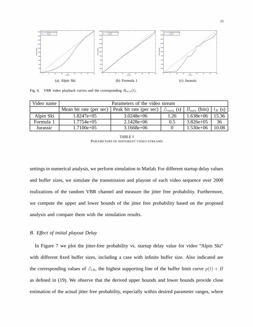
Figure 6 shows the playback curves p(t) for the first 40 seconds of three video sequences and

their corresponding Rbest(t) values. Some main statistics of these video clips, pertinent to the

computation of jitter-free probability bounds, are listed in Table I. These sequences were encoded

at a constant frame rate of 25 frames per second in the Quarter Common Intermediate Format

(QCIF) resolution (176×144). We have chosen the QCIF format because we are particularly

interested in wireless networking systems where hand-held wireless devices typically have a

screen size that corresponds to the QCIF video format.

For numerical analysis, we adopt a three-state extended Gilbert model (e.g., k = 2), with

state transition probabilities Pr{0|1} = 0.005, Pr{0|10} = 0.9 and Pr{0|00} = 0.95. We set

the packet size to be 3600 bits and the time interval between two consecutive transmissions as

20 ms. This results in a maximum transmission bit rate of 180,000 bit/s. Clearly the numerical

results scale correspondingly to networks with different transmission rates. Corresponding to the

23

0 5 10 15 20 25 30 35 400

200

400

600

800

1000

1200

1400

1600

1800

2000

Time (s)

Dat

a (p

acke

ts)

Playback curve p(t)R

best(t)

(a) Alpin Ski

0 5 10 15 20 25 30 35 400

200

400

600

800

1000

1200

1400

1600

1800

2000

Time (s)

Dat

a (p

acke

ts)

Playback curve p(t)R

best(t)

(b) Formula 1

0 5 10 15 20 25 30 35 400

200

400

600

800

1000

1200

1400

1600

1800

2000

Time (s)

Dat

a (p

acke

ts)

Playback curve p(t)R

best(t)

(c) Jurassic

Fig. 6. VBR video playback curves and the corresponding Rbest(t).

Video name Parameters of the video streamMean bit rate (per sec) Peak bit rate (per sec) �min (s) Bmin (bits) tB (s)

Alpin Ski 1.8247e+05 3.0248e+06 1.26 1.638e+06 15.36Formula 1 1.7754e+05 2.1428e+06 0.5 3.826e+05 36Jurassic 1.7100e+05 3.1668e+06 0 1.530e+06 10.08

TABLE IPARAMETERS OF DIFFERENT VIDEO STREAMS

settings in numerical analysis, we perform simulation in Matlab. For different startup delay values

and buffer sizes, we simulate the transmission and playout of each video sequence over 2000

realizations of the random VBR channel and measure the jitter free probability. Furthermore,

we compute the upper and lower bounds of the jitter free probability based on the proposed

analysis and compare them with the simulation results.

B. Effect of initial playout Delay

In Figure 7 we plot the jitter-free probability vs. startup delay value for video “Alpin Ski”

with different fixed buffer sizes, including a case with infinite buffer size. Also indicated are

the corresponding values of �B, the highest supporting line of the buffer limit curve p(t) + B

as defined in (19). We observe that the derived upper bounds and lower bounds provide close

estimation of the actual jitter free probability, especially within desired parameter ranges, where

24

the startup delay is small to moderate and the jitter-free probability is high. Similar results are

observed for different playback curves and omitted to reduce redundancy. The proposed analysis

can be used to derive design guidelines for better segmentation of streaming video to allow more

precise analysis of the jitter probability. As it is mentioned in section III-C, the exact value of

the gap between the upper and lower bounds largely depends on the precise statistics of the

channel curve and the playback curve. The full statistics are usually unavailable to a system

designer in practise, and the modeling of channels and playback curves are outside the scope of

this paper.

We note that, when � ≤ �B , the finite buffer case and the infinite buffer case are nearly the

same, and the jitter free probability increases as � increases. This is because when � ≤ �B,

as we can infer from Figure 4, R(t) will always stay below RB(t), so there will not be any

overflow, and jitter is only induced by underflow. A larger � reduces the probability of underflow.

However, after � surpasses �B, the jitter free probability first increases, but by only a very

small amount, and then decreases as � increases. This is because when � > �B , overflow

occurs. And since the buffer size is fixed, a longer startup delay will result in accumulating too

much data and hence increasing the probability of overflow. When � becomes larger, overflow

starts to dominant and the jitter free probability goes to zero.

The practical implication of the above observation is clear. The initial playout delay is a

delicate parameter in the optimal design of multimedia streaming. Increasing the initial playout

delay can drastically improve the jitter-free probability, but only up to a point determined by

the playback curve and the receiver buffer size. Beyond that point, increasing the initial playout

delay can in fact significantly increase playout jittering. In this regard, the proposed analysis

framework provides a means to accurately estimate the optimal value of the initial playout delay.

25

0 2 4 6 8 10 12 14 16 180

0.1

0.2

0.3

0.4

0.5

0.6

0.7

0.8

0.9

1

Startup Delay Δ (s)

Jitte

r−F

ree

Pro

babi

lity

Simulation πLower Bound π

l

Upper Bound πu

(a) B=2,880 Kbits, �B=8.16s

0 2 4 6 8 10 12 14 16 180

0.1

0.2

0.3

0.4

0.5

0.6

0.7

0.8

0.9

1

Startup Delay Δ (s)

Jitte

r−F

ree

Pro

babi

lity

Simulation πLower Bound π

l

Upper Bound πu

(b) B=3,240 Kbits, �B=10.16s

0 2 4 6 8 10 12 14 16 180

0.1

0.2

0.3

0.4

0.5

0.6

0.7

0.8

0.9

1

Startup Delay Δ (s)

Jitte

r−F

ree

Pro

babi

lity

Simulation πLower Bound π

l

Upper Bound πu

(c) B=3,600 Kbits, �B=12.16s

0 2 4 6 8 10 12 14 16 180

0.1

0.2

0.3

0.4

0.5

0.6

0.7

0.8

0.9

1

Startup Delay Δ (s)

Jitte

r−F

ree

Pro

babi

lity

Simulation πLower Bound π

l

Upper Bound πu

(d) B=∞

Fig. 7. Jitter free probability vs. startup delay with different receiver buffer sizes for video “Alpin Ski”. With 90% confidenceintervals for 2000 runs.

C. Effect of Receiver Buffer Size

Figure 8 shows the effect of receiver buffer size on the jitter-free probability for video “Alpin

Ski” given different startup delay values. It can be seen in this figure that the jitter-free probability

π increases quite fast as the buffer size B increases at first and then after B surpasses a certain

value, π is approximately constant. Thus, increasing the receiver buffer will not necessarily result

in drastically improved performance.

26

1.5 2 2.5 3 3.5 4

x 106

0

0.1

0.2

0.3

0.4

0.5

0.6

0.7

0.8

0.9

1

B (bit)

Jitte

r−F

ree

Pro

babi

lity

Simulation πLower Bound π

l

Upper Bound πu

(a) �=4 s

1.5 2 2.5 3 3.5 4

x 106

0

0.1

0.2

0.3

0.4

0.5

0.6

0.7

0.8

0.9

1

B (bit)

Jitte

r−F

ree

Pro

babi

lity

Simulation πLower Bound π

l

Upper Bound πu

(b) �=6 s

1.5 2 2.5 3 3.5 4

x 106

0

0.1

0.2

0.3

0.4

0.5

0.6

0.7

0.8

0.9

1

B (bit)

Jitte

r−F

ree

Pro

babi

lity

Simulation πLower Bound π

l

Upper Bound πu

(c) �=8 s

1.5 2 2.5 3 3.5 4

x 106

0

0.1

0.2

0.3

0.4

0.5

0.6

0.7

0.8

0.9

1

B (bit)

Jitte

r−F

ree

Pro

babi

lity

Simulation πLower Bound π

l

Upper Bound πu

(d) �=10 s

Fig. 8. Jitter free probability vs. buffer size with different startup delays for video “Alpin Ski”. With 90% confidence intervalsfor 2000 runs.

Furthermore, we note that for a given initial delay �, there exists a maximum buffer size

Bmax(�) = maxt

{min{bmax(t + �), p(L)} − p(t)} (38)

such that for any B ≥ Bmax(�), π is constant:

π = Pr{R(t) ≥ p(t) ∀ t ≤ L}. (39)

The idea is that since R(t) ≤ bmax(t + �) for all t, if RB(t) ≥ bmax(t + �), overflow will not

27

0.90.9

0.9

0.9

0.9

0.99

0.99

0.99

0.99

0.999

0.999

Startup Delay Δ (s)

Buf

fer

Siz

e B

(bi

t)

min Δ →

min B↓

← min αΔ+(1−α)B

6 8 10 12 14 16

2.6

2.8

3

3.2

3.4

3.6

3.8

4

4.2

x 106

(a) Alpin Ski

0.9

0.9

0.9

0.99

0.99

0.999

Startup Delay Δ (s)

Buf

fer

Siz

e B

(bi

t)

4 5 6 7 8 9 10 11 121

1.5

2

2.5x 10

6

(b) Formula 1

0.90.9

0.9

0.99

0.99

Startup Delay Δ (s)

Buf

fer

Siz

e B

(bi

t)

4 5 6 7 8 9 102

2.5

3

3.5

4

4.5

5x 10

6

(c) Jurassic

Fig. 9. Contour maps of buffer size vs. startup delay, with jitter-free probabilities labelled on the curves.

occur and only underflow contributes to jitter, which is equivalent to the infinite buffer case.

Clearly, in terms of resource allocation, hardware implementation, and energy consumption

cost, a smaller buffer size is preferred in practice. Therefore, the proposed analytical framework,

allowing numerical results such as those presented in Figure 8, can provide a means for a first

step toward quantifying the most sensible buffer sizes for optimal system design, taking into

consideration different system cost factors.

D. Optimal Delay-Buffer Tradeoff

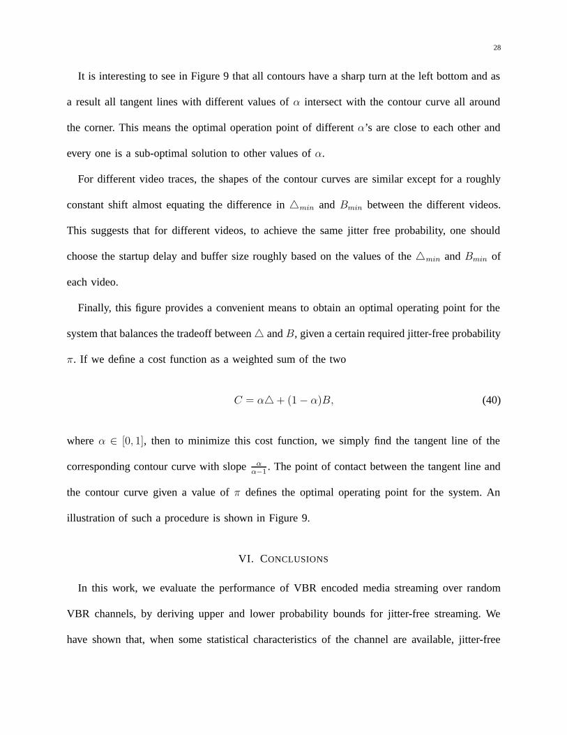
Finally, we consider the optimal tradeoff between the initial playout delay � and the receiver

buffer size B in jitter-free streaming. Figure 9 shows the contour maps of the startup delay and

the buffer size that achieve different jitter free probabilities, for the three video clips described

above.

We observe that the right branch of a contour curves have a slope roughly equal to bmax, the

maximum transmission rate of the channel. This corresponds to the fact that as � increases,

regardless the boundary effect, Bmax(�) increase at rate bmax. This confirms our previous

observation that, in order to achieve π → 1 for a given delay �, we should have B → Bmax(�).

28

It is interesting to see in Figure 9 that all contours have a sharp turn at the left bottom and as

a result all tangent lines with different values of α intersect with the contour curve all around

the corner. This means the optimal operation point of different α’s are close to each other and

every one is a sub-optimal solution to other values of α.

For different video traces, the shapes of the contour curves are similar except for a roughly

constant shift almost equating the difference in �min and Bmin between the different videos.

This suggests that for different videos, to achieve the same jitter free probability, one should

choose the startup delay and buffer size roughly based on the values of the �min and Bmin of

each video.

Finally, this figure provides a convenient means to obtain an optimal operating point for the

system that balances the tradeoff between � and B, given a certain required jitter-free probability

π. If we define a cost function as a weighted sum of the two

C = α� + (1 − α)B, (40)

where α ∈ [0, 1], then to minimize this cost function, we simply find the tangent line of the

corresponding contour curve with slope αα−1

. The point of contact between the tangent line and

the contour curve given a value of π defines the optimal operating point for the system. An

illustration of such a procedure is shown in Figure 9.

VI. CONCLUSIONS

In this work, we evaluate the performance of VBR encoded media streaming over random

VBR channels, by deriving upper and lower probability bounds for jitter-free streaming. We

have shown that, when some statistical characteristics of the channel are available, jitter-free

29

streaming can be achieved with high probability by selecting appropriate initial playout delay

values and receiver buffer sizes.

We have presented a novel analytical framework that only requires knowledge of the play-

back curve, the maximum channel bit rate, and general statistics of the channel, to derive the

probability bounds for jitter-free streaming, for both the infinite buffer and finite buffer cases.

We demonstrate the application of this analytical framework in a wireless access network with

a general extended Gilbert model and ARQ error control. Numerical and experimental results

using MPEG-4 encoded VBR video traces validate our findings.

The computed bounds allow precise estimation of the effects of initial playout delay and

receiver buffer size on streaming performance, especially within system parameter ranges that

lead to sensible jitter-free probabilities. To a practical streaming system designer, the proposed

analysis technique provides a convenient framework to balance the tradeoffs between the initial

playout delay, the receiver buffer size, and the jitter free probability for optimal VBR media

streaming over random VBR channels.

REFERENCES

[1] M. Etoh and T. Yoshimura, “Advances in wireless video delivery,” Proc. IEEE, vol. 93, no. 1, pp. 111–122, January 2005.

[2] T. V. Lakshman, A. Ortega, and A. Reibman, “Vbr video: Trade-offs and potentials,” Proc. IEEE, vol. 86, no. 1, pp.

952–973, May 1998.

[3] S. Sen, J. L. Rexford, J. K. Dey, J. F. Kurose, and D. F. Towsley, “Online smoothing of variable-bit-rate streaming video,”

IEEE Trans. Multimedia, vol. 2, no. 1, pp. 37–48, March 2000.

[4] P. Thiran, J.-Y. L. Boudec, and F. Worm, “Network calculus applied to optimal multimedia smoothing,” in Proc. IEEE

Infocom, April 2001.

[5] V. Varsa and I. Curcio, “Transparent end-to-end packet switched streaming service (pss); rtp usage model (release 5),”

3GPP TR 26.937 V1.4.0, 2003.

30

[6] T. Stockhammer, H. Jenkac, and G. Kuhn, “Streaming video over variable bit-rate wireless channels,” IEEE Trans.

Multimedia, vol. 6, no. 2, pp. 268–277, April 2002.

[7] M. Kalman, E. Steinbach, and B. Girod, “Adaptive media playout for low-delay video streaming over error-prone channels,”

IEEE Trans. Circuits and Systems for Video Technology, vol. 14, no. 6, pp. 841–851, June 2004.

[8] E. N. Gilbert, “Capacity of a burst-noise channel,” Bell Syst. Tech. J., vol. 39, no. 5, pp. 1253–1265, October 1960.

[9] E. O. Elliott, “Estimates of error rates for codes on burst-noise channels,” Bell Syst. Tech. J., vol. 42, pp. 1977–1997, 1963.

[10] P. A. Chou and Z. Miao, “Rate-distortion optimized streaming of packetized media,” Microsoft Research Tech. Rep. MSR-

TR-2001-35, February 2001.

[11] J. Chakareski, P. A. Chou, and B. Girod, “Rate-distortion optimized streaming from the edge of the network,” in Proc.

IEEE Fifth Workshop on Multimedia Signal Processing, December 2002.

[12] H. Seferoglu, Y. Altunbasak, O.Gurbuz, and O. Ercetin, “Rate distortion optimized joint arq-fec scheme for real-time

wireless multimedia,” in Proc. IEEE ICC, May 2005.

[13] H. Sanneck, G. Carle, and R. Koodli, “A framework model for packet loss metrics based on loss run length,” in Proceedings

of SPIE/ACM SIGMM Multimedia Computing and Networking Conference, January 2000.

[14] A. Kpke, A. Willig, and H. Karl, “Chaotic maps as parsimonious bit error models of wireless channels,” in Proc. IEEE

Infocom, March 2003.

[15] A. Willig, “A new class of packet- and bit-level models for wireless channels,” in Proc. 13th IEEE Int. Symp. Personal

Indoor and Mobile Radio Communication (PIMRC), 2000.

[16] H. S. Wang and N. Moayeri, “Finite state markov channel - a useful model for radio communications channels,” IEEE

Trans. Veh. Technol., vol. 44, no. 1, pp. 163–171, 1995.

[17] M. Hassan, M. M. Krunz, and I. Matta, “Markov-based channel characterization for tractable performance analysis in

wireless packet networks,” IEEE Trans. Wireless Commun., vol. 3, no. 3, pp. 821–831, 2004.

[18] F. Fitzek and M. Reisslein, “Mpeg-4 and h.263 video traces for network performance evaluation,” IEEE Network, vol. 15,

no. 6, pp. 40–54, November 2001.