1

Dynamic Processing Allocation in VideoDaozheng Chen, Mustafa Bilgic, Lise Getoor, and David Jacobs

Department of Computer ScienceUniversity of Maryland, College Park

Abstract

Large stores of digital video pose severe computational challenges to existing video analysis algorithms. Inapplying these algorithms, users must often trade-off processing speed for accuracy, as many sophisticated andeffective algorithms require large computational resources that make it impractical to apply them throughout longvideos. One can save considerable effort by applying these expensive algorithms sparingly, directing their applicationusing the results of more limited processing. We show how to do this for retrospective video analysis by modelinga video using a chain graphical model and performing inference both to analyze the video and to direct processing.To accomplish this, we develop a new algorithm to direct processing. This algorithm approximates the optimalsolution efficiently. We apply our algorithm to problems in background subtraction and face detection and show inexperiments that this leads to significant improvements over baseline algorithms.

Index Terms

Video processing, resource allocation, graphical models, optimization, background subtraction, face detection,dynamic programming

I. INTRODUCTION

New technology is giving rise to large stores of digital video. Their size has increased much faster thanthe computational resources needed to effectively process them. At the same time, as we develop increas-ingly sophisticated and effective vision algorithms, these also demand greater computational resources.Consequently, it is important to develop strategies for applying vision algorithms with greater efficiencyto video data.

The scope of the problems we face is evident. Surveillance systems can contain thousands of camerasand a large amount of video. Real time processing of huge data sets is extremely challenging; retrospectiveor forensic analysis creates even greater problems when one must rapidly examine hours or days of videofrom thousands of cameras. For example, British police were required to examine 80,000 CCTV tapesfrom a network of 25,000 cameras [1] to discover the image of a bomber after the terrorist attack inLondon in 2005 [2]. Automatic processing is needed to speed up this analysis, but one cannot hope toprocess all available video in such cases; it is essential to direct processing to portions of video mostlikely to be informative.

In this paper, we develop a new method for controlling processing, so that available resources aredirected at the most relevant portions of the video. In our proposed approach, we initially perform someinexpensive processing of a video by applying a cheap but less accurate algorithm combined with sparseapplication of a more expensive and accurate algorithm. We then use an inference algorithm to determineto which frames we should apply further expensive processing.

Our first contribution is to combine information from cheap and expensive features, using a graphicalmodel for video. This is a second-order Markov model with a node for each frame, and a state variablethat indicates whether this frame is relevant to our current query. For example, the state might indicatewhether the frame contains a visible face. Each state has two potential observations. The first observationis always given; it is obtained by running a cheap algorithm on all frames. For example, cheap backgroundsubtraction might provide a clue as to whether people are currently visible. The second observations isonly obtained if a more expensive and accurate algorithm is applied to that frame (in this example, a facedetector). As in a Hidden Markov Model (HMM), each observation directly depends on the current state.

2

In addition, in our model each observation directly depends on the previous observation. This capturesthe phenomenon that errors made by an algorithm are often correlated from one state to the next. Thismodel allows us to effectively combine information from cheap and expensive algorithms to improveperformance.

Our second and primary contribution is a new algorithm that uses this model to determine where in avideo to apply the expensive algorithm. We build on prior work by Krause and Guestrin [3] that showsthat one can use a dynamic programming algorithm to determine the optimal places at which to makeobservations in a first-order Markov chain. While this work is readily extended to our graphical model,it requires O(B2n3) computation time, where n is the number of nodes in the Markov chain, and B isthe number of places at which we will apply the expensive algorithm. In our setting n is the number offrames in the video and B is also O(n), so this algorithm is not practical for video analysis.

We solve this problem with a new algorithm that produces an approximately optimal answer efficiently.More precisely, we make an additional assumption about the convexity of the reward from observationsas the budget increases, a law of diminishing returns that we show is valid in practice. Then, we showthat by applying part of the total budget to make observations at a uniform step size, we can find a batchallocation of observations that will be at least as good as the optimal allocation, and that requires a modestamount of computation. This batch allocation makes use of rewards computed by Krause and Guestrin’salgorithm, applied to small sections of the video.

Our approach is quite general, and can be applied to a wide range of scenarios in which multiplealgorithms are combined into a single system. Our final contribution is to experimentally demonstratethe value of this algorithm in two very different vision tasks: background subtraction and face detection.First, to perform background subtraction efficiently we combine a very cheap background subtractionalgorithm that uses frame differencing [4] with a more expensive background subtraction algorithm usingGaussian mixture models [5]. Second, we use background subtraction to trigger face detection. We showthat our algorithm can be used to significantly improve performance of systems that combine thesealgorithms. In particular, our inference algorithm requires the idealized assumption that the expensivealgorithm determines the state perfectly. This is never true in practice, but we show that in real-lifesettings this assumption holds sufficiently well that our algorithm produces excellent results. We alsoshow that a relatively poor cheap algorithm can be effectively combined with an expensive algorithm toimprove system performance.

The organization of our paper is as follows. In Section II we discuss related work. In particular, wedescribe a dynamic programming algorithm [3] that determines the optimal place to make observations.We then describe our new algorithm in the context of Markov Chains in section III. Then, we introduceour graphical model for video analysis and describe how to apply the new algorithm to this model insection IV. In section V, we show experiments in video processing.

II. PRIOR WORK

In this section we first review background subtraction and face detection algorithms that are used in ourexperiments. Next, we describe work on video processing that deals with issues of resource constraint.We then discuss work on feature and label acquisition. Finally, we describe the algorithm by Krause andGuestrin [3] in detail.

A. Background SubtractionBackground subtraction is a technique to detect moving objects in video, usually taken by static cameras.

This typically involves building a background model to classify whether a pixel is in the background ornot. We describe two methods in detail since our experiments use these two techniques.

In frame differencing (FD), the background model of the frame at time t, ft, is the frame in the previoustime step, ft−1 (Jain and Nagel [4]). Given a threshold, Th,

|ft − ft−1| > Th (1)

3

gives the foreground region of ft. This technique may not be able to identify the interior pixel of a largeand uniformly-colored moving object. However, it requires very little computation.

Stauffer and Grimson [6] use a mixture of Gaussians (MoG) for the background model of each pixel.Let ~x be the value of the pixels, with the assumption that each dimension of ~x is independent. Theprobability distribution of ~x is modeled as

P (~x) =M∑k=1

ωkN(~µk, σkI), (2)

where M is the number of Gaussian components, ωk is the weight of the kth component, N(~µk, σkI)is a Gaussian distribution with mean ~µk and covariance matrix σkI , where I is the identity matrix. Thismodel is for both foreground and background pixel values. With the assumption that higher and morecompact distribution is more likely to be the background, MoG selects components whose ratio betweenits peak value and standard deviation is greater than a certain threshold. Finally, it uses pixel values from areasonable period of recent time to update the model parameters. A pixel value is assigned to a componentby an on-line K-means approximation and the parameters, ωk, ~µk, and σk are updated by some onlinecumulative average formulas. This method is much more sophisticated than the FD method, and requiressignificantly more computational resources. Zivkovic [5] improves this work by using recursive equationsthat can also simultaneously select the appropriate number of components in the mixture model for eachpixel. We call this method the improved adaptive Gaussian mixture model (IAGMM), and we use it inour experiments.

B. Face DetectionFace detection refers to the problem of determining whether an image contains faces, and determining

the location and extent of each faces. Yang et al. [7] provide a comprehensive survey of various facedetection methods. Of these methods, we describe the work by Viola and Jones [8] in detail because ourexperiment uses this technique.

Viola and Jones introduce a now widely used object detection scheme, applying it first to face detection.With integral images for fast computation, they use a set of feature that are similar to the coefficients inHaar wavelet transforms. They then construct classifiers by selecting a small number of important featuresusing Adaboost. Finally, the scheme detects faces inside an image region by applying classifiers in acascade. At each level of the cascade, one uses a classifier with a very low false negative rate, althoughfalse positives might be high. Subsequent classifiers are run only when previous classifiers indicate apositive result. One can think of this as a methodology for combining classification algorithms, which isalso our topic. However, while very effective, this approach requires a variety of cheap classifiers with arange of performance characteristics, and is hard to apply when one wishes to combine the results of afew specific algorithms. Lienhart and Maydt [9] extend this work by adding an efficient set of 45◦ rotatedfeatures to the original feature set and by using a new post-optimization procedure for a given boostedclassifier. Their work shows significantly lower false alarm rate, and we use this method to detect facesin our experiment.

C. Computational Performance in Video ProcessingThere is a vast literature on video processing. Performance is often an issue, as many effective algorithms

are too slow to run in real-time, and even fast algorithms may require enormous amounts of time whenused to perform retrospective analysis of large quantities of previously taken video. One common strategyis to run cheap, lower level algorithms such as motion detectors to determine when something interestingmight be happening. When these detect motion, higher level algorithms are then deployed. In a variantof this, Krishna et al. [10] propose an algorithm switching approach to handle background subtraction.The system starts by processing each frame with a uni-modal background subtraction algorithm. When

4

the system shows poor segmentation quality, it switches to use the MoG model. The system considerswhen to apply the expensive algorithm in real time, and it simulates the trigger of algorithm switch froman external source, such as a motion sensor or a light sensor.

Barotti et al. [11] present a closely related work that uses algorithm switching to handle lightingchanges and solve bootstrapping problems in motion detection. When the system detects sudden globalillumination variation, the motion detection switches from background subtraction using a single Gaussianto FD. The latter algorithm requires smaller computational resources, adapts quickly to lighting changes,and does not need any bootstrapping. The system then re-initializes the single Gaussian model to handlethe bootstrapping problem, and returns to the original configuration when initialization completes. Thiswork uses the advantages of the cheap algorithm to handle the drawbacks of the expensive algorithm ina particular application.

An alternative approach is to use special-purpose hardware or high performance computing to runexpensive algorithms efficiently. A number of researchers consider using graphics hardware to acceleratecomputer vision algorithms. For example, real-time stereo algorithms suitable for implementation onGraphics Processing Units (GPU) are proposed in [12], [13], and [14]. Yang and Welch [15], and Griesseret al. [16] introduce algorithms to do background subtraction in real time using a GPU. Heymann et al.[17] and Sinha et al. [18] use a GPU to detect and track image feature points in real time. Fung et al. [19]introduce openVIDIA which provides a library and API for using single or multiple GPUs to acceleratecomputer vision and image processing. Besides GPUs, there are many other hardware solutions to efficientcomputation of expensive algorithms. For instance, implementations of image feature detectors using aField-programmable gate array (FPGA) are discussed in [20] and [21]. Seinstra et al. [22] introduceParallel-Horus which allows researchers in multimedia content analysis to implement sequential programsin Grid computing environment.

In general, while these methods are of interest, they are largely orthogonal to our concerns in this paper.In particular, if we can gain greater efficiency by directing processing of expensive algorithms in a video,these can be readily combined with hardware solutions that speed up these algorithms.

D. Feature and Label AcquisitionIn closely related work, the machine learning community has looked at the problem of determining

which features to acquire in order to correctly classify instances. In this setup, instances are describedby a set of features each of which has an associated acquisition cost, and a total budget limits featureacquisition. Some example strategies are [23], [24]. The biggest difference between this line of work andours is that the feature-value acquisition community treats each instance as independent; the decisions forone instance are made independent of the decisions made for the other instances. However, in our case,the information we want to extract in nearby frames of video is highly correlated, and we should be ableto do better if we take these correlations into account.

Another related area of work is label acquisition: instead of obtaining features, we can query an oracleto determine an instance’s label directly. Given a network of instances, such as a sequence of frames, anetwork of friends, etc, acquiring the label for an instance helps in correctly classifying the rest of thenetwork. The question is then which instances should be queried in order to get the best performance onthe remaining ones. Rattigan et al. [25] queries the instances that are structurally important, e.g. highlyconnected instances, central instances, etc. Bilgic and Getoor [26] build a classifier that can predict whichinstances might be misclassified and query a central instance only if it is predicted as misclassified. Eventhough these methods have been quite successful in practice, they are heuristic approaches and have notheoretical guarantees (partly because they are applicable to general networks). However, for the class ofchain graphical models such as HMMs, Krause and Guestrin [3] show how to solve the label acquisitionproblem optimally. We describe their work next.

5

E. Optimal Observation PlansKrause and Guestrin [3] present an optimal algorithm for selecting observations for the class of chain

graphical models. Since we build on this method, we now describe it in some detail, although we considera special case of their work that is suitable to our problem. A set of random variables S = {X1, · · · , Xn}forms a chain graphical model if whenever i < j < k, Xi is conditionally independent of Xk given Xj .For example, consider a HMM unrolled for n time slices. Then the n hidden state variables form a chaingraphical model. Suppose that for each of these variables, it is possible to observe its hidden state at afixed cost. This corresponds, in our problem, to the supposition that an expensive algorithm is extremelyaccurate, and reveals the hidden state. They also suppose that observing variable Xj has a local rewardRj . In particular, the expected local reward is

Rj(Xj|O) ,∑o

P (O = o)Rj(P (Xj|O = o)), (3)

which is an expectation taken over all possible values o for the observed variables O. Many differentfunctions, such as entropy, are applicable for this local reward. They describe the max-marginal:

Rj(Pmax(Xj|O)) =

∑o

P (o)[Pmax(x∗j |o)− Pmax(xj|o)], (4)

where xj is the value of state variable Xj , x∗ = argmaxxjPmax(xj|o), and x = argmaxxj 6=x∗P

max(xj|o).This reward is very useful for classification purposes [3], and we use it in all examples and experimentin this paper. In our case, since we have a two-class problem, this reward is equivalent to considering theexpected number of correct classifications.

Assume that there is a fixed budget B for selecting observations, the formulation of the optimizationproblem is:

Select observations to maximize

J(O) = R(O) =∑j

Rj(Xj|O) (5)

Subject to

b ≤ B (6)

where j is the index over the state variables S, b is the number of observed state variables O, and Bis the total budget for the whole chain. Also, observations can include variables at any time step in thechain since we consider processing a video after it is recorded. Krause and Guestrin refer to this as thesmoothing problem.

In addition, the conditional independence property in the chain graphical model simplifies the localreward. With this property, the local reward is simply R(Xj|O) = R(Xj|Xj) in the case that Xj ∈ O. Inthe case that Xj is not in O, we have R(Xj|O) = R(Xj|Oj), where Oj is the subset of O containing theclosest ancestor and descendant of Xj in O. This is the key insight for efficiently solving this optimizationproblem.

Furthermore, they consider both a conditional planning version of this problem, in which the bestobservation is made and then the optimal next observation is computed, and this is repeated k times, anda batch version of the problem, in which one decides on the locations of the best observations with atotal cost of k first, and then makes these observations. We only consider the conditional planning varianthere since it in general produces the best performance.

Krause and Guestrin [3] solve this problem by noting that once an observation is made, it splits theproblem of determining future observations into conditionally independent components before and afterthe observations. This allows for a dynamic programming solution. They define a value, Ja:b(xa, xb; k)

6

which denotes the reward produced by the optimal plan with a budget of k over the interval from variablesXa to Xb, given that these variables have been observed to have states xa and xb. Then they note thatJa:b(xa, xb; k) can be recursively computed given the value of Jc:d(xc, xd; l) for all a ≤ c ≤ d ≤ b andl < k. For the case of smoothing and conditional planning, the recursive formula is

Ja:b(xa, xb; k) = max{Ja:b(xa, xb; 0), maxa<j<b

{∑xj

P (Xj = xj|Xa = xa, Xb = xb){

Rj(Xj|Xj = xj) + max0≤l≤k−1

[Ja:j(xa, xj; l) + Jj:b(xj, xb; k − l − 1)]}}}, (7)

where the base case is

Ja:b(xa, xb; 0) =b−1∑

j=a+1

Rj(Xj|Xa = xa, Xb = xb). (8)

To handle the case that Xa and Xb are not always observed in advance, the algorithm adds two independentdummy variables, Xa−1 and Xb+1, which have no reward and observation cost but have default states, tothe head and tail positions of the chain. Thus the optimal reward for a chain of n variables with a budgetof B is computed as J0:n+1(x0, xn+1;B). Assuming that the probabilities to evaluate local rewards havebeen computed and computing local rewards takes constant time, we conclude from Theorem 2 in [3]that the complexity of this algorithm is

O(B2n3). (9)

III. EFFICIENT OBSERVATION PLANS FOR CHAIN GRAPHICAL MODELS

We now present a novel algorithm to find observation plans that is efficient enough to apply to problemswith very large values of n. While the new algorithm only approximates the optimal one, it is much fasterfor domains such as ours. In the next sections, we will show how this algorithm can be applied to videoprocessing. Our algorithm first uses part of the total budget to make uniform observations with a certainstep size. This splits the Markov chain into M consecutive intervals where the first and last variables ofeach interval are observed. Because of the Markov assumption of the chain model, this breaks our problemup into a series of smaller problems of the same size. These problems are not independent, however, sincethe remaining budget must be parceled out between all these intervals. We show that, with an additional,reasonable assumption, this can be done optimally. Once the budget is allocated to intervals, observationscan be allocated within intervals using the optimal algorithm of Krause and Guestrin. The main novelinsight of this approach is that rather than just allocating observations to optimize reward, in practice itmay make sense to allocate some observations in a way that makes the inference algorithm more tractable.

This leads to Algorithm 1, Dynamic Processing Allocation (DPA), which is something of a hybridbetween conditional and batch allocation. Such a strategy uses a budget of size B′+B′′ and is guaranteed

Algorithm 1 Dynamic Processing Allocation (DPA)1) We use B′ observations to make uniform observations to break the chain model into consecutive

disjoint intervals separated by the observed variables;2) We allocate the remaining budget B′′ to these intervals in a batch mode;3) We use the optimal observation algorithm in section II-E to determine the observation locations

within each interval in a conditional mode.

to perform at least as well as an optimal batch algorithm that uses a budget of size B′′. In practice, weexpect to do much better than this optimal batch algorithm, since the observations we use to break theproblem into intervals also provide very useful information, and because we can use an optimal conditionalplan within each interval, which can be much better than the optimal batch plan.

In step 2 of the algorithm, which allocates the budget between intervals, we consider maximizing thesum of optimal reward across all intervals. That is, let ki be the budget allocated to interval i and Ji(ki)

7

be the reward of the optimal plan for interval i with a budget of ki. We want to find k1, k2, · · · , and kMsuch that they maximize

M∑i=1

Ji(ki), (10)

subject toM∑i=1

ki = B′′. (11)

To do this optimization, we observe that for each interval, the optimal reward typically forms a convexcurve as the budget increases. That is, for internal i, the plot of Ji(ki) against ki as ki increases is convexin general. This means that we suppose function Ji(ki) exhibits submodularity, which is a kind of law ofdiminishing returns property: Adding additional observations helps less if many observations have alreadybeen made and helps more if only a few observations have been made [27]. We denote these kinds ofcurves as Reward-Budget (RB) curves, and the assumption that these curves are convex will allow us tooptimally allocate our budget. We will experimentally verify that this assumption is reasonable.

We now introduce an algorithm to maximize the sum of reward increments for each interval. Let Ni

be the maximum budget allowed for interval i, typically the number of unobserved state variables in theinterval. We define the reward increment with budget k as

∆Ji(k) ≡ Ji(k)− Ji(k − 1), (12)

where k = 1, · · · , Ni. Given the convexity assumption, we have

∆Ji(k) ≤ ∆Ji(k − 1) (13)

for all possible ks, and we denote this as the convexity property. With this notation, we describe Algorithm2, batch budget allocation. In practice, most intervals are allocated small budgets, so it is wasteful to

Algorithm 2 Batch budget allocation1) Compute the reward increment ∆Ji(k) for i = 1, 2, · · · ,M with all possible ks;2) Sort all these reward increments in descending order. Then the budget for each interval is determined

by the number of increments it has in the top B positions of the sorted list.

compute the entire RB curve for all these intervals. We therefore can use Algorithm 3, incremental budgetallocation, to do the optimization and save running time.

Algorithm 3 Incremental budget allocation1) Initialize the budget of each interval to be zero;2) Compute the reward increment ∆Ji(1) for i = 1, 2, · · · ,M ;3) Select the highest increment, and add one to the budget of the corresponding interval I;4) If the total budget for the whole chain has been used up, terminate and use the current budget

allocation for each interval as the final budget allocation;5) If not, compute the next reward increment for interval I, and use it to replace the current reward

increment for this interval. Go back to step 4.

8

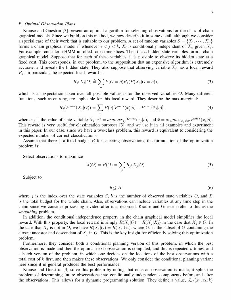
Fig. 1. The example chain graphical model. Because we assume that X1 and X9 are observed in advance, we use gray nodes withdouble-line boundaries to highlight this. The state of a node can be 1 or 2, and we show the actual state on the top of each node.

A. An ExampleWe use an example to illustrate how DPA works and how the optimal algorithm is different from ours.

Consider a chain graphical model with nine state variables whose value can be either 1 or 2. The priorprobability of being in each state is 0.5. The transition probability of switching from one state to the otheris 0.2. Figure 1 shows this model and it displays the states on the top of each variable. For simplicity, weassume the first and last states are known in advance. Fig. 2 shows how DPA with batch budget allocationand how the optimal algorithm determine the observation locations with a budget of 4.

First, we note that for this example, it is most likely that the initial states have a value of 1, andthat at some point in the chain there is a single transition from 1 to 2. To correctly determine the statevalues, the main goal is to find the location of this transition. It is also possible that there are really threetransitions from 1 to 2 to 1 to 2, and a secondary goal will be to check on that. Next, we note that theoptimal conditional plan is able to perform a binary search to find such transitions. The optimal strategyfor this situation involves first determining the value of X3. If this state is 1, then the remaining budgetis sufficient to allow a binary search to be performed on states X4-X8, to find the transition from 1 to2. This strategy therefore guarantees that the transition from 1 to 2 will be found, and maximizes thechances that any additional transitions will be found.

Suppose instead we run DPA, with a budget of 4. In this case, the algorithm must begin by determiningthe state of X5, to break the problem into two equal parts. When this state is found to be 1, the algorithmthen allocates its budget between these two subsequences. To allocate the remaining budget to eachinterval, it computes the RB curves up to its maximum budget for both intervals, as shown in Fig. 2(c)and 2(d). Notice that both curves satisfy the convexity property. In addition, the reward increment undera small budget for the right interval is higher than those for the left interval. This is because the state ofthe first and last nodes for the right interval indicate a state transition in between. As a result, the rightinterval obtains a higher budget. In fact, DPA allocates two observations to the right side of the chain,which is enough to perform a binary search for the state transition, and one observation to the left side.This final observation on the left side is more likely to find something interesting than if allocated to theright side, once the binary search has occurred.

Notice that DPA is not optimal in two ways. First, an optimal set of observations may not include X5.Second, allocating one observation to the left subsequence and two to the right subsequence may notbe optimal; future observations could determine that a different allocation would be better. On the otherhand, in the optimal algorithm shown in Fig. 2(b), notice that the initial observation X3 is determinedafter computation and comparison of expect reward of observing X1, · · · , X9 with all possible budgetdistribution. This is a considerable amount of computation. In DPA, this interval is split into two shorterintervals, and reward can be more cheaply computed for each subchain separately.

Finally, we consider how incremental budget allocation works in this example in detail. After theobservation of X5, the chain is split into two intervals as shown in Fig. 2(a) and the remaining budgetbecomes 3. The incremental algorithm then initializes the budget for both intervals to be 0 and computesJ1(0), J1(1), J2(0), and J2(1) for ∆J1(1) and ∆J2(1). Since ∆J1(1) = 0.3626 < ∆J2(1) = 1.0000,it increases the budget for the right interval by 1. The remaining budget becomes 2 and it computesJ2(2) for ∆J2(2). After this, it again increases the budget for the right interval by 1 because ∆J1(1) <∆J2(2) = 1.0000. The remaining budget becomes 1 and it computes J2(3) for ∆J2(3). After this, because∆J1(1) > ∆J2(3) = 0.1176, it increases the budget for the left interval by 1. The remaining budget

9

(a) DPA with batch budget allocation (b) Optimal algorithm

(c) RB curve - interval 1 (left interval) (d) RB curve - interval 2 (right interval)

Fig. 2. (a) shows how DPA with batch budget allocation determines the observation locations. We use gray color to highlight observed nodes.The interval size is 5, so the initial observation is X5, which is highlighted by a double-line boundary with a thick inner line. (c) and (d) showthe RB curves for left and right intervals respectively. The observation locations for each of these two intervals are determined by the optimalalgorithm, and are highlighted by a single-line thick boundary. (b) shows how the optimal algorithm determines observations locations, whichare also highlighted by a single-line thick boundary. It shows how the chain is split into sub-chains by sequential observations.

10

becomes 0 and the algorithm terminates with budget of 1 for left interval and 2 for the right interval.Notice that compared with batch allocation, incremental allocation saves computation by not computingJ1(2) and J1(3).

B. Proof of CorrectnessWe now provide a proof that batch budget allocation is correct; it follows directly that incremental

budget allocation must also be correct.We use the following new notations, definitions, and facts. With a budget of B, we let kB1 , k

B2 , · · · , kBM

be an optimal budget allocation, where M indicates the number of subsequences among which we mustdivide the budget. Let kB1 , k

B2 , · · · , kBM be the budget allocation by the algorithm. Denote the sorted list

rewards gained by an additional observation as Z and the sum of the top B reward increments in Z as∆L. In addition, we define ∆Ji(0) ≡ 0 to handle the case that some interval has a budget of 0. Then wedefine ∆JBi ≡

∑kBij=0 ∆Ji(j), which means ∆JBi is the sum of all reward increments for interval i with a

budget of kBi . Similarly, we define ∆JBi ≡∑kB

ij=0 ∆Ji(j). Furthermore, since the algorithm pick only top

B reward increments from Z to distribute budget, it is clear that∑M

i=1 kBi = B. Therefore, to prove the

correctness, we only need to show that∑M

i=1 Ji(kBi ) =

∑Mi=1 Ji(k

Bi ). We now use Lemma 1, Lemma 2,

and Theorem 1 to prove this.Lemma 1:

M∑i=1

∆JBi = ∆L. (14)

Proof: For an interval i, by the procedure of the algorithm, there must be kBi reward incrementsfrom interval i in ∆L. Let the sum of these increments be ∆Li. In case that no such increment exists, welet ∆Li ≡ 0. Suppose ∆JBi 6= ∆Li. By convexity property, we know that ∆Li must include some rewardincrement ∆Ji(x) such that x > kBi and ∆Ji(x) < ∆Ji(k

Bi ) ≤ ∆Ji(k

Bi − 1) ≤ · · · ≤ ∆Ji(1). Thus, there

must be at least kBi + 1 reward increments in top B positions from interval i. But this conflicts with thefact that the top B positions only contain kBi such increments. Thus, it can only be that ∆JBi = ∆Li.Finally, because

∑Mi=1 k

Bi = B, we have

∑Mi=1 ∆Li = ∆L. Therefore,

∑Mi=1 ∆JBi =

∑Mi=1 ∆Li = ∆L.

Lemma 2:M∑i=1

∆JBi ≥M∑i=1

∆JBi . (15)

Proof: For any reward increment which is outside the top B positions of Z, we know it must beless than or equal to any reward increment within the top B positions because Z is sorted in descendingorder. Therefore, by Lemma 1,

∑Mi=1 ∆JBi = ∆L must be greater than or equal to the sum of any B

reward increments from Z. Because∑M

i=1 kBi = B and list Z contains the all possible reward increments

from all intervals, we know that∑M

i=1 ∆JBi is also the sum of B reward increments from Z. Therefore,∑Mi=1 ∆JBi ≥

∑Mi=1 ∆JBi .

By the definition of ∆Ji(k), we know that Ji(k) = ∆Ji(k) + Ji(k− 1). Using induction, it is trivial toshow that Ji(k) =

∑kj=1 ∆Ji(j) + Ji(0). Because we define ∆Ji(0) ≡ 0, then

Ji(k) =k∑j=0

∆Ji(j) + Ji(0). (16)

With this formula, we can finally prove the correctness in following theorem.Theorem 1:

M∑i=1

Ji(kBi ) =

M∑i=1

Ji(kBi ). (17)

11

Proof: By equation (16), we have

M∑i=1

Ji(kBi ) =

M∑i=1

[

kBi∑

j=0

∆Ji(j) + Ji(0)] =M∑i=1

[∆JBi + Ji(0)] =M∑i=1

∆JBi +M∑i=1

Ji(0). (18)

Similarly,M∑i=1

Ji(kBi ) =

M∑i=1

∆JBi +M∑i=1

Ji(0). (19)

Then by lemma 2, it follows that∑M

i=1 Ji(kBi ) ≥

∑Mi=1 Ji(k

Bi ). Finally, because the budget allocation,

kB1 , kB2 , · · · , kBM , is optimal, we have

∑Mi=1 Ji(k

Bi ) =

∑Mi=1 Ji(k

Bi ).

C. Complexity AnalysisWe can now determine the complexity of DPA. Here we consider the cost of determining where to

make additional observations, where the cost of making each observation is always the cost of runningthe expensive algorithm. We introduce the following notation. Let the total budget be B = B′ + B′′ andlet ε be a number less than 1 such that

n

M=

1

ε. (20)

Since each interval has the same length, this is 1ε. In addition, because the first step of the algorithm uses

B′ budget to make observations at a uniform step size, we have B′ = M = εn (we choose ε so that εnis an integer).

The first step of DPA takes O(B′) = O(εn) running time, since these observations are at fixed locationswith uniform step size. For the second step, using batch budget allocation, we need to compute the RBcurve for each interval up to its maximum budget, which is in O(1

ε). Following the asymptotic result of

(9), the running time to compute these curves is

O(M · (1

ε)2(

1

ε)3) = O(εn · (1

ε)5) = O(

1

ε4n). (21)

Since producing the sorted list and picking the reward in the top positions takes O(nlog(n)) time, thetotal running time is

O(1

ε4n+ nlog(n)). (22)

Using incremental budget allocation, we only need to compute the RB curve for each interval up to itsallocated budget. Thus, the complexity is

O(M∑j=1

(k2j (

1

ε)3)) = O(

1

ε3

M∑j=1

k2j ), (23)

where kj is the allocated budget for interval j. Because∑M

j=1 kj = B′′ and kj ≤ 1ε

for all j,∑M

j=1 k2j

reaches its maximum by letting as many intervals have budget 1ε

as possible. For each of the other intervals,it either has 0 budget or has the remaining of the total budget. As a result, the number of intervals thathave nonzero budget is dB′′/1

εe = O(B′′/1

ε) = O(εB′′). Thus, we further conclude that

O(1

ε3

M∑j=1

k2j ) = O(

1

ε3· εB′′ · (1

ε)2) = O(

1

ε4B′′) (24)

In addition, we must also maintain a sorted list of the incremental rewards from computing RB curvesfor each interval as budget increases. Using data structures such as a binary heap [28], we can build an

12

(a) (b)

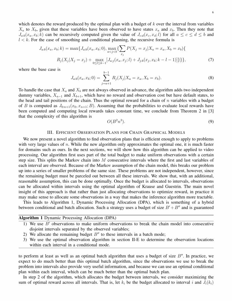
Fig. 3. Markov models for video frame sequences. (a) The model we use when expensive feature is not available at every frame; (b) Themodel we use when all frames have expensive features.

initial sorted list in O(Mlog(M)) = O(B′log(B′)) time, and then add and remove B′′ increments to thatlist in O(B′′log(B′)) time. This gives a total running time of:

O(1

ε4B′′ + (B′ +B′′)log(B′) = O(

1

ε4B +Blog(B)). (25)

Finally, the last step involves using the optimal algorithm for each interval to determine the additionalsampling locations. This takes O(B′′) running time given dynamic programming memory tables for eachinterval in the budget allocation stage. However, storing all the tables for each interval require a largeamount of memory space. Alternatively, we can rerun the optimal algorithm for each interval using theallocated budget, which gives an additional run time of O( 1

ε4n) for batch allocation, and O( 1

ε4B′′) for

incremental allocation. Finally, the total running time is

O(εn+1

ε4n+ nlog(n) +

1

ε4n) = O(εn+

2

ε4n+ nlog(n)) = O(

1

ε4n+ nlog(n)) (26)

for batch budget allocation, and is

O(B′ +1

ε4B +Blog(B) +

1

ε4B) = O(B +

2

ε4B +Blog(B)) = O(

1

ε4B +Blog(B)) (27)

for incremental budget allocation. This is a vast improvement over O(B2n3) for the optimal algorithm.In our experiments, we show that this computation is quite practical.

IV. DATA FUSION FOR FRAME SEQUENCES

In this section, we first describe how we model the frame sequence from a video as a graphical modelfor data fusion in section IV-A. This model is a Markov chain which emits cheap and expensive features.Therefore, we can apply DPA to this model and section IV-B describes this. Finally, we discuss on howto run the forward-backward algorithm for this model in section IV-C.

A. A Graphical Model for Frame SequencesThe graphical model is a Markov model, where each frame of video corresponds to a node. Each node

contains a state variable that represents the property we wish to infer, such as whether a face, or a movingobject, is present. Each node can emit two observable quantities, corresponding to cheap and expensivefeatures extracted from the frame. This is similar to a hidden Markov model (HMM), but here we alsomodel dependencies between observations. In our model, the value of a cheap feature at time t is notconditionally independent of the rest of the model given the state at time t, but is also dependent on thecheap feature at times t−1 and t+1. We do this to capture the fact that when a feature makes an error inone frame, it is quite likely to make a similar error at an adjacent frame. (Note if we assume conditional

13

independence among features at different time steps, it results in less accurate inference performance).This model can be considered a type of autoregressive hidden Markov model [29], or conditional randomfield [30].

However, we typically have expensive features for a small fraction of frames, so it is not trivial tomodel the dependency between them. In addition, we assume the expensive feature is accurate whenpredicting the state. Therefore, we do not model the dependency between expensive features, and makeit only depend on the state. However, in the case that we have an expensive feature at every frame, wemodel the dependency the same as with cheap features. We illustrate these two cases in Figure 3. Statevariables are labeled “X”, cheap observations are labeled “c”, and expensive observations are labeled “e”.They all have numbered subscripts indicating their time steps.

B. Applying DPAWe have described DPA for the case of simple, chain graphical models. However, it is straightforward

to apply it to the model in previous section, since it has a chain structure and the same conditionalindependence property. Specifically, to apply DPA to our model we first treat the chain formed by thestate variables in our model as the chain graphical model. Second, assuming that the expensive featureis accurate in predicting the state, we consider the places to reveal states in the chain as the locationsto sample expensive feature. And we use the predicted states to compute the optimal reward describedin section. Finally, cheap feature also provides useful information. Thus, we make the recursive formulasfor computing the optimal reward be conditioned on applicable cheap features. Denoting ca:b as the cheapfeature over the interval from variable Xa and Xb, the formula (7) and (8) for computing the optimalreward become

Ja:b(xa, xb; k) = max{Ja:b(xa, xb; 0), maxa<j<b

{∑xj

P (Xj = xj|Xa = xa, Xb = xb, ca:b){

Rj(Xj|Xj = xj, ca:b) + max0≤l≤k−1

[Ja:j(xa, xj; l) + Jj:b(xj, xb; k − l − 1)]}}}, (28)

where the base case is

Ja:b(xa, xb; 0) =b−1∑

j=a+1

Rj(Xj|Xa = xa, Xb = xb, ca:b). (29)

C. Forward-backward AlgorithmWhen using formula (28) and (29) to determine where to sample expensive features, and using our

model to do inference to predict the state of each frame, we need to determine the probability distributionof each state based on observations. We can use the Forward-Backward algorithm [31] to do this. Usingour model, this algorithm works a little differently from the standard version, due to dependencies in theobservations, and we describe it below. The derivation uses the ideas in [29] and [32].

Let N be the number of states, and denote individual states as S = {s1, s2, · · · , sN}. Let the sequencehave T time slices. Also let cheap feature observations from time 1 to T be c1, c2, · · · , cT respectively,and expensive feature observations from time 1 to T be e1, e2, · · · , eT . Let fi be {ci, ei} at time i and Obe all the observations. Similarly, we use Xt to denote the state variable at time t. Then,

P (Xt = si|O) =P (O,Xt = si)

P (O)=P (f1···T , Xt = si)

P (O)

=P (ft+1···T |Xt = si, f1···t)P (Xt = si, f1···t)

P (O)

∝ P (ft+1···T |Xt = si, ft)P (Xt = si, f1···t). (30)

14

Given the forward variable defined as αt(i) = P (Xt = si, f1···t) and the backward variable as βt(i) =P (ft+1···T |Xt = si, ft), we have

P (Xt = si|O) ∝ αt(i) · βt(i). (31)

To compute αt(i), we have

αt(i) = P (Xt = si, f1···t) = P (Xt = si, ft, f1···t−1)

= P (Xt = si, ft|f1···t−1)P (f1···t−1)

=N∑j=1

P (Xt = si, ft|Xt−1 = sj, f1···t−1)P (Xt−1 = sj|f1···t−1)P (f1···t−1)

=N∑j=1

P (ft|Xt−1 = sj, f1···t−1, Xt = si)P (Xt = si|Xt−1 = sj, f1···t−1)P (Xt−1 = sj, f1···t−1)

=N∑j=1

P (ft|f1···t−1, Xt = si)P (Xt = si|Xt−1 = sj)P (Xt−1 = sj, f1···t−1)

=N∑j=1

P (ft|f1···t−1, Xt = si)P (Xt = si|Xt−1 = sj)αt−1(j), (32)

where P (ft|f1···t−1, Xt = si) = P (ct|ct−1, Xt = si)P (et|Xt = si) for the left model and P (ft|f1···t−1, Xt =si) = P (ct|ct−1, Xt = si)P (et|et−1, Xt = si) for the right model in Fig. 3. This gives the recursive formulato compute the forward variable, where the base condition is the same as that in [31]. The only differencefrom the standard forward algorithm is that the probability of the observation needs to be conditioned onthe observation in the previous time step.

To compute βt(i), we have

βt(i) = P (ft+1···T |Xt = si, ft) =N∑j=1

P (ft+2···T , Xt+1 = sj, ft+1|Xt = si, ft)

=N∑j=1

P (ft+2···T |Xt+1 = sj, ft+1, Xt = i, ft)P (Xt+1 = sj, ft+1|Xt = si, ft)

=N∑j=1

P (ft+2···T |Xt+1 = sj, ft+1)P (ft+1|Xt+1 = sj, ft)P (Xt+1 = sj|Xt = si)

=N∑j=1

βt+1(j)P (Xt+1 = sj|Xt = si)P (ft+1|Xt+1 = sj, ft), (33)

where P (ft+1|Xt+1 = sj, ft) = P (ct+1|Xt+1 = sj, ct)P (et+1|Xt+1 = sj) for the left model and P (ft+1|Xt+1 =sj, ft) = P (ct+1|Xt+1 = sj, ct)P (et+1|Xt+1 = sj, et) for the right model in Fig. 3. Again, the onlydifference from the standard backward algorithm is that probability of the observation is conditioned onthe observation in the previous time step.

V. EXPERIMENTS

We now apply DPA to two vision tasks involving motion detection and face detection. Our main goal isto show that inference can be used to efficiently allocate processing in two very different tasks. We beginby first describing some common characteristics of our experiments in the next section. We then presentthe results for the two tasks in section V-B and V-C. Section V-D and V-E discuss how the expensive andcheap features can affect DPA. Finally, section V-F discusses the running time.

15

A. General Experiment SetupFor DPA, given a video with n frames and a budget of B = B′ + B′′, we first use B′ budget to run

the expensive algorithm uniformly with a step size of 20, while also running the cheap algorithm on allframes. Then we use the batch budget allocation to distribute the remaining budget B′′ among intervals,which are separated by frames whose state is predicted by the expensive feature. This step gives us abudget for each interval, and we use the optimal algorithm to determine where to observe expensivefeatures within each interval. For convenience of description, we describe budget in term of its percentageof the total number of frames.

One assumption in this budget allocation method is that the reward curve as the budget increases isconvex for the subsections. To evaluate this assumption, we compute the RB curve for each intervalup to its maximum budget. For those curves which are not strictly convex, the difference between twoconsecutive reward increments must be positive at some points. We pick the highest such value as thenonconvexity measure of a RB curve, and find that this measure is typically very small. So we approximateeach nonconvex RB curve with a convex curve, which yields a good approximation. Section V-B and V-Cgive more details on the nonconvexity measure.

When running DPA, we also assume that the expensive algorithm always correctly reveals the state ofa frame. This is not really true, so we expect that occasional errors made by an expensive algorithm willcause us to allocate resources suboptimally. However, since our inferences will in general be correct, westill expect DPA to produce decisions that are effective overall.

Finally, when all observations have been made, we predict the state of each frame using the inferencemodel in Fig. 3(a) since expensive features are not available in every frame. We compared our results toseveral baseline algorithms. Competing algorithms are always provided the same total budget for a faircomparison.• The first baseline method is uniform sampling, which runs the expensive algorithm at a uniform step

size. This method is in essence equivalent to running the expensive algorithm at a lower frame rate.• The second baseline method is most-relevant sampling. In this sampling method, we first run the

cheap algorithm at each frame and perform inference using the model in Fig. 3(a) to obtain theconditional probabilities of the state variables at each frame. We then run the expensive algorithm onthe frames that are most likely to satisfy our query. This is equivalent to using the cheap algorithmto prune the least interesting frames.

• The third and last baseline method is most-uncertain sampling. Similar to the most-relevant samplingmethod, we again run the cheap algorithm at each frame and then perform inference to obtainconditional probabilities. Then, we run the expensive algorithm on frames that have the greatestuncertainty. Uncertainty can be measured in many ways. For example, we can use entropy of theconditional probability, or we can use 1 - maximum conditional probability. For binary classificationtasks such as ours here, both choices produce an identical ranking. The motivation behind thissampling strategy is that we want to invest resources at locations we are most uncertain about.

• Finally, to calibrate the performance of algorithms on different tasks, we compared to an idealizedmethod, ceiling sampling, in which we run the cheap and expensive algorithms at all the frames, i.e,the budget is equal to 100%. We use Fig. 3(b) to model the frame sequence because the expensivefeature is available everywhere. This method should provide an upper bound on the performance ofany method given that the model fits the data well enough.

To compare these methods, we used 4-fold cross validation on each video, using three-quarters of thedata to train the model and one quarter to evaluate the model. We recorded each video in 30 frame persecond. We then uniformly sampled 3 frames per second to generate the training and testing sequences,and this is a reasonable frame rate to experiment on for real world surveillance videos. By beginningsampling at different locations, we produced 10 different sequences for training and also for testing. Allten sequences are used as training data. We also use all ten for testing, helping to smooth the results a bit.The performance measure we used was the 11-point average precision of the precision recall (PR) curves

16

[33]. That is, we take the average precision for 11 uniformly spaced levels of recall. This is averagedover all 40 testing sequences from the 4 folds.

For the first three sampling methods, we ran the cheap algorithm at each frame and ran the expensivealgorithm only at the sampled locations. For ceiling sampling, we ran the expensive algorithm on all frames.We combined the cheap and expensive features and performed inference using the models illustrated inFig. 3. We used the conditional probabilities for each frame’s state variable to generate PR curves. Themethods differed only in their choice of where to apply the expensive algorithm, and use the samealgorithm to do inference. To compare the sampling methods under varying conditions, we varied thetotal budget from 5% to 25% of n. We next provide more details about the experiments for both tasks.

B. Motion DetectionWe first evaluated these algorithms in a simple background subtraction task. We collected three half

hour videos at thirty frames per second, for a total of n ≈ 55, 000 per video, with each frame at 240×320resolution. We hand-labeled each frame as “interesting” if it contained a moving object, such as a personor car, “uninteresting” otherwise.

As a cheap algorithm, we used FD [4] and we used IAGMM [5] as the expensive algorithm. Usingthe first algorithm, the feature was the number of foreground pixels in a frame after applying a thresholdof 10. This avoided postprocessing, saving a significant amount of computational resources. It is aninteresting question for future work to determine how best to build a background model suitable for theexpensive algorithm based on sparsely sampled frames. However, in this experiment we wish to focus onthe effectiveness of our algorithm in directing application of IAGMM. Therefore, we build a backgroundmodel using all recent frames and then apply IAGMM only at sampled locations. After applying theIAGMM, we performed an opening and a closing morphological operation. We then extracted the largestconnected component to generate features, which were discretized to run the experiment. We had used8 different features, which included the area of the component, the width of its Bounding Box, and thediameter of a circle with the same area as the component. They all produced similar performance, andwe chose the area of the component to show results. Figure 4 shows some frame examples and thecorresponding output by FD and IAGMM algorithms.

Next, we tested our convexity assumption on these videos, since DPA assumes that the reward curveswere convex. Table I shows the results. We can see that over a half of all intervals produce convex rewardcurves, while most of the non-convex ones have very small concavities.

TABLE I

CONVEXITY OF RB CURVES FOR THE MOTION DETECTION TASKS

Video Video 1 Video 2 Video 3Number of intervalsb 2720 2720 2720Convex (%) 56.21 67.39 59.93Convex or ≈ convexb(%) 94.34 97.28 94.45Median of the restc 0.0468 0.0181 0.0834a The total number of intervals over the 40 testing sequences.b RB curves which are not convex but with nonconvexity

measure not greater than 0.01.c The median of nonconvexity measure for those intervals

which are neither convex or ≈ convex.

We show 11-point average precision results on the three videos in Fig. 5. In all three videos, our methodoutperforms the baseline methods. We also observe from the plots that uniform sampling outperforms bothmost-relevant sampling and most-uncertain sampling. We postulate that the reason may be that the cheapalgorithm does not produce high quality features and so decisions based purely on the cheap algorithmare unreliable. In these videos, FD faces difficulties because leaves often move in the background.

17

Video 1

Video 2

Video 3

Fig. 4. Frame examples from video 1, 2, and 3 for the motion detection task and their corresponding output from the cheap and expensivealgorithms. Within each video, the first row shows the original frame, the second and the third rows show the corresponding output from FDand IAGMM respectively. FD tends to produce more noise for foreground pixels which affects accuracy of features. IAGMM gives muchfewer false positives, and in general produce better feature for detection.

18

Fig. 5. 11-point average precision values for the background subtraction task.

C. Face DetectionNext, we applied our approach to the problem of identifying frames containing a face. As with the last

task, we collected three half-hour videos. We hand-labeled each frame as “interesting” if there is a frontalor profile face in it and labeled it as “uninteresting” otherwise.

For the cheap algorithm, we used IAGMM with the area of the largest connected component as a featuresince it is relatively good at detecting the motion of a human and is still computationally cheap comparedto the face detector. The expensive algorithm was the face detection algorithm based on OpenCV [34],using the scheme in [9]. We used both frontal and profile face detectors and the expensive feature wasa binary indicator of whether the detectors found a face. Fig. 6 shows frame examples from these threevideos.

TABLE II

CONVEXITY OF RB CURVES FOR THE FACE DETECTION TASK.

Video video 4 video 5 video 6Number of subsections 2720 2840 2800Convex (%) 80.22 66.16 68.61Convex or ≈ convex (%) 98.16 98.45 99.07Rest median 0.0970 0.1014 0.1014

We again first measured the convexity of the reward curves for the face detection videos. The results aregiven in Table II. Again, the reward curves are largely convex. We show the 11-point average precisionresults on the three videos in Figure 7. Our method outperforms the baseline methods in two videos, video4 and 5, under all budget percentages. However, in video 6, our method has no advantage over uniformsampling when the budget is small, but as the budget increases, the advantage of our method becomesclear.

D. Accuracy of Expensive FeaturesThe accuracy of the expensive feature can cause variations in performance of DPA, since our decisions

are based on the assumption that the expensive feature is very accurate. To see this, we measured theprediction error rates of the expensive feature on all six videos. Remember that our method is guaranteedto be optimal when the expensive feature determines the correct state perfectly, and our graphical model

19

Video 4

Video 5

Video 6

Fig. 6. Example frames from video 4, 5, and 6 for the face detection task and their corresponding output from the cheap and expensivealgorithms. Within each video, the first row shows the original frame, the second and the third rows show the corresponding output fromIAGMM and face detectors respectively. IAGMM produces information about whether moving objects, such as humans, are present or not,while face detectors give explicit knowledge about presence of faces.

20

Fig. 7. 11-point average precision values for the face detection task.

correctly models the domain. The prediction error rates of the expensive feature in the six videos are.0153, .0421, .0395, .0587, .0830, and .2328 respectively. Note that the error rate is highest in the sixthvideo, the video on which our method has no clear advantage over uniform sampling when given a smallbudget.

E. Usefulness of Cheap FeaturesIdeally, combining both features to guide DPA to determine the expensive feature sampling locations

should give better result than purely using expensive feature. However, we observe that when the modeldoes not fit the dependency properties of the domain, combining both features can actually hurt per-formance of DPA. To show this, we replace the cheap feature with a constant synthetic feature. Underthis setting, the sampling locations and inference only depends on the expensive features. We compareperformance of these two cases. Following the similar setup above, we observe that combining bothfeatures has a clear advantage over only using the expensive feature. Fig. 8 shows the result.

However, we do observe that when we vary the frame rates, purely using expensive features can havebetter performance than combining both features. Fig. 9 shows the performance when the frame rate is 30,6, 2, and 1. When the frame rate is 30 or 6 frame per second, combining both features has no advantageover using purely expensive features. In particular, using purely expensive features has better performancefor the first three videos for background subtraction task under 30 frames per second. However, when theframe rate is 2 or 1 frame per second, the advantage of combining both feature becomes clear again. This isvery likely due to the issue that how well our model fits the data. When the frame rate becomes higher andhigher, the dependency between the cheap features is stronger and stronger, and our model cannot capturethis well enough. As a result, the cheap feature is overconfident in some locations, and suppresses thecorrect decisions by the expensive features. Using a better model that captures this dependency adequatelyis one way to deal with this problem, however it adds significant computational complexity. Furthermore,real world videos, such as surveillance videos, need to run for a long time in general. A small frame rateis more suitable for storage and power issues [35]. Combining both features is good in this case. At thesame time, we stress that in situations in which cheap features are not helpful, DPA will still providesignificant benefits, using only expensive features to control processing.

F. Running TimeFinally, we discuss the processing overhead of DPA. Without considering the feature generation time,

which is application dependent, the main processing time of DPA is at the stage of determining expensive

21

Fig. 8. Comparison of using cheap features from real data and constant synthetic cheap features under frame rate of 3 frame per second.

features sampling locations. With unoptimized MATLAB and Java code and without considering thefeature generation time, DPA requires an average of 7.6 seconds to handle one-fourth of a half-hourvideo when the budget is 5% at 3 frames per second. And it needs about 9.7 seconds when the budgetis 25%. This overhead is small compared with the time to record the video. However, when the framerate is 30 frames per second, the average running time becomes 76.3 seconds when the budget is 5%and 97.0 seconds when the budget is 25%. Both the length of a testing sequence and the running time inthe later case is 10 times longer than those in former case. With a fixed interval size, the running timegrows linearly as the testing frame sequence grows. However, we see that the computational overhead isrelatively small compared with the video recording time. For real world applications, in which the framerate needs to be small to save computational resource, DPA will in particular be useful.

VI. CONCLUSION

Our main goal has been to design inference algorithms that can be used to direct video processing.This allows us to replace simplistic methods such as reducing the frame rate with principled decisionsthat carry theoretical performance guarantees. We believe that this is a quite general framework that canbe applied to many video processing tasks and may be extended in the future to more complex graphicalstructures.

To this end, we have made two more detailed contributions. First, we propose a graphical model thatmaps onto a video frame sequence and allows us to combine features from expensive and cheap algorithmsto do inference. We show that in practical situations, there is much to be gained by this combination.Second, we have shown how to build on an existing algorithm that was designed for short chains tocreate an algorithm that runs efficiently on long video sequences. Specifically, we show that by applyingan expensive algorithm in some extra locations, we can control additional applications of the algorithm

22

Fig. 9. Comparison of using cheap features from real data and constant synthetic cheap features under frame rate of 30, 15, 5, and 1 frameper second. From top to bottom, each row shows the results for all videos under a frame rate, from 30 to 1 frame per second.

with significantly smaller running time. Experiments with two concrete video processing tasks, low-levelbackground subtraction and the higher level task of face detection, show that these can be mapped ontoour framework. The effectiveness of DPA’s inference algorithm in these tasks illustrates the potential ofour approach for general video processing.

REFERENCES

[1] L. Telindus Surveillance Systems, “http://www.telindussurveillance-us.com/,” 2005.[2] N. Dean, “Bombers staged dry run before london attacks,” The Independent, online edition, 20 Sept. 2005.[3] A. Krause and C. Guestrin, “Optimal nonmyopic value of information in graphical models - efficient algorithms and theoretical limits,”

in International Joint Conference on Artificial Intelligence, 2005.[4] R. Jain and H. Nagel, “On the analysis of accumulative difference pictures from image sequences of real world scenes,” IEEE

Transactions on Pattern Analysis and Machine Intelligence, vol. 1, pp. 206–213, 1979.[5] Z. Zivkovic, “Improved adaptive gaussian mixture model for background subtraction,” in International Conference on Pattern

Recognition, 2004.[6] C. Stauffer and W. Grimson, “Adaptive background mixture models for real-time tracking,” IEEE Conference on Computer Vision and

Pattern Recognition, 1999.[7] M. hsuan Yang, D. J. Kriegman, S. Member, and N. Ahuja, “Detecting faces in images: A survey,” IEEE Transactions on Pattern

Analysis and Machine Intelligence, vol. 24, pp. 34–58, 2002.[8] P. Viola and M. Jones, “Robust real-time object detection,” International Journal of Computer Vision, vol. 57, pp. 137–154, 2002.

23

[9] R. Lienhart and J. Maydt, “An extended set of haar-like features for rapid object detection,” in IEEE International Conference on ImageProcessing, 2002.

[10] R. Krishna, K. McCusker, and N. O’Connor, “Optimising resource allocation for background modeling using algorithm switching,” inACM/IEEE International Conference on Distributed Smart Cameras, 2008.

[11] S. Barotti, L. Lombardi, and P. Lombardi, “Multi-module switching and fusion for robust video surveillance,” in International Conferenceon Image Analysis and Processing, 2003.

[12] R. Yang and M. Pollefeys, “Multi-resolution real-time stereo on commodity graphics hardware,” in IEEE Conference on ComputerVision and Pattern Recognition, 2003.

[13] C. Zach, K. Karner, and H. Bischof, “Hierarchical disparity estimation with programmable 3d hardware,” in International Conferencein Central Europe on Computer Graphics, Visualization and Computer Vision, 2004.

[14] J. Woetzel and R. Koch, “Real-time multi-stereo depth estimation on GPU with approximative discontinuity handling,” in EuropeanConference on Visual Media Production, 2004.

[15] R. Yang and G. Welch, “Fast image segmentation and smoothing using commodity graphics hardware,” Journal of Graphics Tools,vol. 7, pp. 91–100, 2002.

[16] A. Griesser, S. D. Roeck, A. Neubeck, and L. V. Gool, “GPU-based foreground-background segmentation using an extended colinearitycriterion,” in International Fall Workshop on Vision, Modeling, and Visualization, 2005.

[17] S. Heymann, K. Maller, A. Smolic, B. Froehlich, and T. Wiegand, “SIFT implementation and optimization for general-purpose GPU,”in International Conference in Central Europe on Computer Graphics, Visualization and Computer Vision, 2007.

[18] S. N. Sinha, J. michael Frahm, M. Pollefeys, and Y. Genc, “GPU-based video feature tracking and matching,” in Workshop on EdgeComputing Using New Commodity Architectures, 2006.

[19] J. Fung and S. Mann, “OpenVIDIA: parallel GPU computer vision,” in Annual ACM International Conference on Multimedia, 2005.[20] C. Cabani and W. J. MacLean, “Implementation of an affine-covariant feature detector in field-programmable gate arrays,” in

International Conference on Computer Vision Systems, 2007.[21] S. Se, T. Barfoot, and P. Jasiobedzki, “Visual motion estimation and terrain modeling for planetary rovers,” in International Symposium

on Artificial Intelligence for Robotics and Automation in Space, 2005.[22] F. J. Seinstra, J.-M. Geusebroek, D. Koelma, C. G. Snoek, M. Worring, and A. W. Smeulders, “High-performance distributed image

and video content analysis with parallel-horus,” IEEE Multimedia, vol. 14, pp. 64–75, 2007.[23] V. Bayer-Zubek, “Learning diagnostic policies from examples by systematic search,” in Conference on Uncertainty in Artificial

Intelligence, 2004.[24] P. D. Turney, “Cost-sensitive classification: Empirical evaluation of a hybrid genetic decision tree induction algorithm,” Journal of

Artificial Intelligence Research, vol. 2, pp. 369–409, 1995.[25] M. Rattigan, M. Maier, and D. Jensen, “Exploiting network structure for active inference in collective classification,” in ICDM Workshop

on Mining Graphs and Complex Structures, 2007.[26] M. Bilgic and L. Getoor, “Effective label acquisition for collective classification,” in International Conference on Knowledge Discovery

and Data mining, 2008.[27] A. Krause, B. McMahan, C. Guestrin, and A. Gupta, “Robust submodular observation selection,” Journal of Machine Learning Research,

vol. 9, pp. 2761–2801, 2008.[28] T. H. Cormen, C. E. Leiserson, R. L. Rivest, and C. Stein, Introduction to Algorithms, Third Edition. Cambridge, MA, USA: The

MIT Press, 2009.[29] K. P. Murphy, “Dynamic bayesian networks: Representation, inference and learning,” Ph.D. dissertation, UC Berkeley, Computer Science

Division, 2002.[30] C. Sutton and A. McCallum, “An introduction to conditional random fields for relational learning,” in Introduction to Statistical

Relational Learning, L. Getoor and B. Taskar, Eds. Cambridge, MA, USA: MIT Press, 2007, pp. 93–127.[31] L. Rabiner, “A tutorial on hidden markov models and selected applications in speech recognition,” Proceedings of the IEEE, vol. 77,

pp. 257–286, 1989.[32] T. Fletcher, “Switching autoregressive hidden markov model,” Department of Computer Science, University College London, Tech.

Rep., 2009.[33] C. D. Manning, P. Raghavan, and H. Schtze, Introduction to Information Retrieval. New York, NY, USA: Cambridge University Press,

2008.[34] Intel, “Opencv open source computer vision library,” http://www.intel.com/technology/computing/opencv/index.htm.[35] C. Loy, T. Xiang, and S. Gong, “Multi-camera activity correlation analysis,” in IEEE Conference on Computer Vision and Pattern

Recognition, 2009.