1

Deep Audio-Visual Speech RecognitionTriantafyllos Afouras, Joon Son Chung, Andrew Senior, Oriol Vinyals, Andrew Zisserman

Abstract—The goal of this work is to recognise phrases and sentences being spoken by a talking face, with or without the audio.Unlike previous works that have focussed on recognising a limited number of words or phrases, we tackle lip reading as an open-worldproblem – unconstrained natural language sentences, and in the wild videos.Our key contributions are: (1) we compare two models for lip reading, one using a CTC loss, and the other using asequence-to-sequence loss. Both models are built on top of the transformer self-attention architecture; (2) we investigate to what extentlip reading is complementary to audio speech recognition, especially when the audio signal is noisy; (3) we introduce and publiclyrelease a new dataset for audio-visual speech recognition, LRS2-BBC, consisting of thousands of natural sentences from Britishtelevision.The models that we train surpass the performance of all previous work on a lip reading benchmark dataset by a significant margin.

Index Terms—Lip Reading, Audio Visual Speech Recognition, Deep Learning.

F

1 INTRODUCTION

L IP READING, the ability to recognize what is being saidfrom visual information alone, is an impressive skill, and

very challenging for a novice. It is inherently ambiguous at theword level due to homophones – different characters that produceexactly the same lip sequence (e.g. ‘p’ and ‘b’). However, suchambiguities can be resolved to an extent using the context ofneighboring words in a sentence, and/or a language model.

A machine that can lip read opens up a host of applications:‘dictating’ instructions or messages to a phone in a noisy environ-ment; transcribing and re-dubbing archival silent films; resolvingmulti-talker simultaneous speech; and, improving the performanceof automated speech recognition in general.

That such automation is now possible is due to two develop-ments that are well known across computer vision tasks: the useof deep neural network models [30, 44, 47]; and, the availabilityof a large scale dataset for training [41]. In this case, the lipreading models are based on recent encoder-decoder architecturesthat have been developed for speech recognition and machinetranslation [5, 7, 22, 23, 46].

The objective of this paper is to develop neural transcription ar-chitectures for lip reading sentences. We compare two models: oneusing a Connectionist Temporal Classification (CTC) loss [22],and the other using a sequence-to-sequence (seq2seq) loss [9, 46].Both models are based on the transformer self-attention architec-ture [49], so that the advantages and disadvantages of the twolosses can be compared head-to-head, with as much of the rest ofthe architecture in common as possible. The dataset developed inthis paper to train and evaluate the models, are based on thousandsof hours of videos that have talking faces together with subtitlesof what is being said.

We also investigate how lip reading can contribute to audiobased speech recognition. There is a large literature on thiscontribution, particularly in noisy environments, as well as the

• T. Afouras and J. S. Chung are with the University of Oxford.E-mail:{afourast,joon}@robots.ox.ac.uk

• A. Senior and O. Vinyals are with Google DeepMind.E-mail:{vinyals,andrewsenior}@google.com

• A. Zisserman is with the University of Oxford and Google DeepMind.E-mail:az@robots.ox.ac.uk

The first two authors contributed equally to this work.

converse where some derived measure of audio can contribute tolip reading for the deaf or hard of hearing. To investigate thisaspect we train a model to recognize characters from both audioand visual input, and then systematically disturb the audio channel.

Our models output at the character level. In the case ofthe CTC, these outputs are independent of each other. In thecase of the sequence-to-sequence loss a language model is learntimplicitly, and the architecture incorporates a novel dual attentionmechanism that can operate over visual input only, audio inputonly, or both. The architectures are described in Section 3. Bothmodels are decoded with a beam search, in which we can option-ally incorporate an external language model.

Section 4, we describe the generation and statistics of a newlarge scale dataset, LRS2-BBC, that is used to train and evaluate themodels. The dataset contains talking faces together with subtitlesof what is said. The videos contain faces ‘in the wild’ with asignificant variety of pose, expressions, lighting, backgrounds andethnic origin. Section 5 describes the network training, where wereport a form of curriculum learning that is used to acceleratetraining. Finally, Section 6 evaluates the performance of themodels, including for visual (lips) input only, for audio and visualinputs, and for synchronization errors between the audio and visualstreams.On the content: This submission is based on the conferencepaper [12]. We replace the WLAS model in the original paper withtwo variants of a Transformer-based model [49]. One variant waspublished in [2], and the second variant (using the CTC loss) is anoriginal contribution in this paper. We also update the visual front-end with a ResNet-based one proposed by [45]. The new front-end and back-end architectures contribute to over 22% absoluteimprovement in Word Error Rate (WER) over the model proposedin [12]. Finally, we publicly release a new dataset, LRS2-BBC,that supersedes the original LRS dataset in [12] which could notbe made public due to license restrictions.

2 BACKGROUND

2.1 CTC vs sequence-to-sequence architecturesFor the most part, end-to-end deep learning approaches for se-quence prediction can be divided into two types.

arX

iv:1

809.

0210

8v2

[cs

.CV

] 2

2 D

ec 2

018

2

Text predictions

Audio

Video

A

V

Language Model

Encoder

Encoder

Decoder Beam Search

Fig. 1: Outline of the audio-visual speech recognition pipeline.

The first type uses a neural network as an emissionmodel which outputs the likelihood of each output symbol(e.g. phonemes) given the input sequence (e.g. audio). Thesemethods generally employ a second phase of decoding using aHidden Markov Model [25]. One such version of this variantis the Connectionist Temporal Classification (CTC) [22], wherethe model predicts frame-wise labels and then looks for theoptimal alignment between the frame-wise predictions and theoutput sequence. The main weakness of CTC is that the outputlabels are not conditioned on each other (it assumes each unitis independent), and hence a language model is employed as apost-processing step. Note that some alternatives to jointly trainthe two step process has been proposed [21]. Another limitationof this approach is that it assumes a monotonic ordering betweeninput and output sequences. This assumption is suitable for ASRand transcription for example, but not for machine translation.

The second type is sequence-to-sequence models [9, 46](seq2seq) that first read all of the input sequence before predictingthe output sentence. A number of papers have adopted thisapproach for speech recognition [10, 11]: for example, Chan etal. [7] proposes an elegant sequence-to-sequence method to tran-scribe audio signal to characters. Sequence-to-sequence decodesan output symbol at time t (e.g. character or word) conditioned onprevious outputs 1, . . . , t − 1. Thus, unlike CTC-based models,the model implicitly learns a language model over output symbols,and no further processing is required. However, it has been shown[7, 26] that it is beneficial to incorporate an external languagemodel in the decoding of sequence-to-sequence models as well.This way it is possible to leverage larger text-only corpora thatcontain much richer natural language information than the limitedaligned data used for training the acoustic model.

Regarding architectures, while CTC-based or seq2seq ap-proaches traditionally relied on recurrent networks, recently therehas been a shift towards purely convolutional models [6]. Forexample, fully convolutional networks have been used for ASRwith CTC [51, 55] or a simplified variant [16, 32, 54].

2.2 Related worksLip reading. There is a large body of work on lip readingusing non deep learning methods. These methods are thoroughlyreviewed in [56], and we will not repeat this here. A numberof papers have used Convolutional Neural Networks (CNNs) topredict phonemes [37] or visemes [29] from still images, asopposed to recognising to full words or sentences. A phonemeis the smallest distinguishable unit of sound that collectively makeup a spoken word; a viseme is its visual equivalent.

For recognising full words, Petridis et al. [39] train an LSTMclassifier on a discrete cosine transform (DCT) and deep bottle-

neck features (DBF). Similarly, Wand et al. [50] use an LSTMwith HOG input features to recognise short phrases. The shortageof training data in lip reading presumably contributes to thecontinued use of hand crafted features. Existing datasets consistof videos with only a small number of subjects, and also a limitedvocabulary (<60 words), which is also an obstacle to progress.Chung and Zisserman [13] tackles the small-lexicon problem byusing faces in television broadcasts to assemble the LRW datasetwith a vocabulary size of 500 words. However, as with any word-level classification task, the setting is still distant from the real-world, given that the word boundaries must be known beforehand.Assael et al. [4] uses a CNN and LSTM-based network and(CTC) [22] to compute the labelling. This reports strong speaker-independent performance on the constrained grammar and 51word vocabulary of the GRID dataset [17].

A deeper architecture than LipNet [4] is used by [45], whopropose a residual network with 3D convolutions to extract morepowerful representations. The network is trained with a cross-entropy loss to recognise words from the LRW dataset. Here, thestandard ResNet architecture [24] is modified to process 3D imagesequences by changing the first convolutional and pooling blocksfrom 2D to 3D.

In our earlier work [12], we proposed a WLAS sequence-to-sequence model based on the LAS ASR model of [7] (theacronym WLAS are for Watch, Listen, Attend and Spell, andLAS for Listen, Attend and Spell). The WLAS model had a dualattention mechanism – one for the visual (lip) stream, and the otherfor the audio (speech) stream. It transcribed spoken sentences tocharacters, and could handle an input of vision only, audio only,or both.

In independent and concurrent work, Shillingford et al. [43],design a lip reading pipeline that uses a network which outputsphoneme probabilities and is trained with CTC loss. At inferencetime, they use a decoder based on finite state transducers to convertthe phoneme distributions into word sequences. The network istrained on a very large scale lip reading dataset constructed fromYouTube videos and achieves a remarkable 40.9% word error rate.Audio-visual speech recognition. The problems of audio-visualspeech recognition (AVSR) and lip reading are closely linked.Mroueh et al. [36] employs feed-forward Deep Neural Networks(DNNs) to perform phoneme classification using a large non-public audio-visual dataset. The use of HMMs together with hand-crafted or pre-trained visual features have proved popular – [48]encodes input images using DBF; [20] used DCT; and [38] usesa CNN pre-trained to classify phonemes; all three combine thesefeatures with HMMs to classify spoken digits or isolated words.As with lip reading, there has been little attempt to develop AVSRsystems that generalise to real-world settings.

Petridis et al. [40] use an extended version of the architectureof [45] to learn representations from raw pixels and waveformswhich they then concatenate and feed to a bidirectional recurrentnetwork that jointly models the audio and video sequences andoutputs word labels.

3 ARCHITECTURES

In this section, we describe model architectures for audio-visualspeech recognition, for which we explore two variants, based onthe recently proposed Transformer model [49]: i) an encoder-decoder attention structure for training in a seq2seq manner andii) a stack of self-attention blocks for training with CTC loss. The

3

3D/2D ResNet

STFT

Feed Forward

x6

Multi-head Attention

Feed Forward

x6

Multi-head Attention Feed Forward

Linear, Softmax

Character Probabilities

Multi-head Attention

Q

x6

b. Transformer seq2seq

Feed Forward

x6

Multi-head Attention

Linear, Softmax

CTC Posterior Probabilities

V A

Multi-head Attention

Multi-head Attention

c. Transformer CTC

Vc Ac

a. Common Encoder

K, VK, V

Q, K, VQ, K, V

Q, K, V

V AQ, K, V

V A

Fig. 2: Audio-visual speech recognition models. (a) Common encoder: The visual image sequence is processed by a spatio-temporalResNet, while the audio features are the spectrograms obtained by applying Short Time Fourier Transform (STFT) to the audio signal.Each modality is then encoded by a separate Transformer encoder. (b) TM-seq2seq: a Transformer model. On every decoder layer,the video (V) and audio (A) encodings are attended to separately by independent multi-head attention modules. The context vectorsproduced for the two modalities, Vc and Ac respectively, are concatenated channel-wise and fed to the feed forward layers. K, V andQ denote the Key, Value and Query tensors for the multi-head attention blocks. For the self-attention layers it is always Q = K = V ,while for the encoder-decoder attentions, K = V are the encodings (V or A), while Q is the previous layer’s output (or, for the firstlayer, the prediction of the network at the previous decoding step). (c) TM-CTC: Transformer CTC, a model composed of stacks ofself-attention and feed forward layers, producing CTC posterior probabilities for every input frame. For full details on the multi-headattention and feed forward blocks refer to Appendix B.

architecture is outlined in Figure 2. The general model receivestwo input streams, one for video (V) and one for audio (A).

3.1 Audio Features

For the acoustic representation we use 321-dimensional spectralmagnitudes, computed with a 40ms window and 10ms hop-length,at a 16 kHz sample rate. Since the video is sampled at 25 fps (40ms per frame), every video input frame corresponds to 4 acousticfeature frames. We concatenate the audio features in groups of 4,in order to reduce the input sequence length as is common forstable CTC training [8, 42], while at the same time achieving acommon temporal-scale for both modalities.

3.2 Vision Module (VM)

The input images are 224×224 pixels, sampled at 25 fps andcontain the speaker’s face. We crop a 112×112 patch covering theregion around the mouth, as shown in Figure 3. To extract visualfeatures representing the lip movement, we use a spatio-temporalvisual front-end that is based on [45]. The network applies 3Dconvolutions on the input image sequence, with a filter width of5 frames, followed by a 2D ResNet that gradually decreases thespatial dimensions with depth. The layers are listed in full detailin Appendix A. For an input sequence of T ×H ×W frames, theoutput is a T× H

32×W32×512 tensor (i.e. the temporal resolution is

preserved) that is then average-pooled over the spatial dimensions,yielding a 512-dimensional feature vector for every input videoframe.

3.3 Common self-attention Encoder

Both variants that we consider use the same self-attention-basedencoder architecture. The encoder is a stack of multi-head self-attention layers, where the input tensor serves as the query, keyand value for the attention at the same time. A separate encoder isused for each modality as shown in Figure 2 (a). The informationabout the sequence order of the inputs is fed to the model via fixedpositional embeddings in the form of sinusoid functions.

3.4 Sequence-to-sequence Transformer (TM-seq2seq)

In this variant, separate attention heads are used for attending onthe video and audio embeddings. In every decoder layer, the re-sulting video and audio contexts are concatenated over the channeldimension and propagated to the feedforward block. The attentionmechanisms for both modalities receive as queries the output ofthe previous decoding layer (or the decoder input in the case ofthe first layer). The decoder produces character probabilities whichare directly matched to the ground truth labels and trained with across-entropy loss. More details about the multi-head attention andfeed-forward building blocks are given in Appendix B.

4

3.5 CTC Transformer (TM-CTC)The TM-CTC model concatenates the video and audio encodingsand propagates the result through a stack of self-attention /feedforward blocks, same as the one used in the encoders. Theoutputs of the network are the CTC posterior probabilities forevery input frame and the whole stack is trained with CTC loss.

3.6 External Language Model (LM)For decoding both variants, during inference, we use a character-level language model. It is a recurrent network with 4 unidi-rectional layers of 1024 LSTM cells each. The language modelis trained to predict one character at a time, receiving onlythe previous character as input. Decoding for both models isperformed with a left-to-right beam search where the LM log-probabilities are combined with the model’s outputs via shallowfusion [26]. More details on decoding are given in Appendices Cand D.

3.7 Single modality modelsThe audio-visual models described in this section can be usedwhen only one of the two modalities is present. Instead of con-catenating the attention vectors for TM-seq2seq or the encodingsfor TM-CTC, only the vector from the available modality is used.

4 DATASET

In this section, we describe the multi-stage pipeline for auto-matically generating a large-scale dataset, LRS2-BBC, for audio-visual speech recognition. Using this pipeline, we have been ableto collect thousands of hours of spoken sentences and phrasesalong with the corresponding facetrack. We use a variety of BBCprograms from Dragon’s Den to Top Gear and Countryfile.

The processing pipeline is summarised in Figure 4. Most ofthe steps are based on the methods described in [13] and [14], butwe give a brief sketch of the method here.

Video preparation. A CNN face detector based on the Single ShotMultiBox Detector (SSD) [33] is used to detect face appearancesin the individual frames. Unlike the HOG-based detector [27] usedby previous works, the SSD detects faces from all angles, andshows a more robust performance whilst being faster to run.

The shot boundaries are determined by comparing color his-tograms across consecutive frames [31]. Within each shot, facetracks are generated from face detections based on their positions,as feature-based trackers such as KLT [34] often fail when thereare extreme changes in viewpoints.

Audio and text preparation. The subtitles in television are notbroadcast in sync with the audio. The Penn Phonetics Lab ForcedAligner [53] is used to force-align the subtitle to the audio signal.Errors exist in the alignment as the transcript is not verbatim –therefore the aligned labels are filtered by checking against thecommercial IBM Watson Speech to Text service.

AV sync and speaker detection. In broadcast videos, the audioand the video streams can be out of sync by up to around one sec-ond, which can cause problems when the facetrack correspondingto a sentence is being extracted. A multi-view adaptation [15] ofthe two-stream network described in [14] is used to synchronisethe two streams. The same network is also used to determinewhich face’s lip movements match the audio, and if none matches,the clip is rejected as being a voice-over.

Sentence extraction. The videos are divided into individualsentences/ phrases using the punctuations in the transcript. Thesentences are separated by full stops, commas and question marks;and are clipped to 100 characters or 10 seconds, due to GPUmemory constraints. We do not impose any restrictions on thevocabulary size.

The LRS2-BBC dataset is divided into development (train/val)and test sets according to broadcast date. The dataset also hasa “pre-train” set that contains sentence excerpts which may beshorter or longer than the full sentences included in the devel-opment set, and are annotated with the alignment boundaries ofevery word. The statistics of these sets are given in Table 1. Thetable also compares the ‘Lip Reading Sentences’ (LRS) seriesof datasets to the largest existing public datasets. In addition toLRS2-BBC, we use MV-LRS and LRS3-TED for training andevaluation.

Datasets for training external language models. To train thelanguage models used for evaluation on each audio-visual dataset,we use a text corpus containing the full subtitles of the videosfrom which the dataset’s training set was generated. The text-onlycorpus contains 26M words.

5 TRAINING STRATEGY

In this section, we describe the strategy used to effectively train themodels, making best use of the limited amount of data available.The training proceeds in four stages: i) the visual front-end moduleis trained; ii) visual features are generated for all the training datausing the vision module; iii) the sequence processing module istrained on the frozen visual features; iv) the whole network istrained end-to-end.

5.1 Pre-training visual featuresWe pre-train the visual front-end on word excerpts from the MV-LRS [15] dataset, using a 2-layer temporal convolution back-endto classify every clip with a word label similarly to [45]. Weperform data augmentation in the form of horizontal flipping,removal of random frames [4, 45], and random shifts of up to ±5pixels in the spatial dimensions and of ±2 frames in the temporaldimension.

5.2 Curriculum learningSequence to sequence learning has been reported to converge veryslowly when the number of timesteps is large, because the decoderinitially has a hard time extracting the relevant information fromall the input steps [7]. Even though our models do not contain anyrecurrent modules, we found it beneficial to follow a curriculuminstead of immediately training on full sentences.

We introduce a new strategy where we start training only onsingle word examples, and then let the sequence length grow asthe network trains. These short sequences are parts of the longersentences in the dataset. We observe that the rate of convergenceon the training set is several times faster, while the curriculum alsosignificantly reduces overfitting, presumably because it works as anatural way of augmenting the data.

The networks are first trained on the frozen features of thepre-train sets from MV-LRS, LRS2-BBC and LRS3-TED. Wedeal with the difference in utterance lengths by zero-padding thesequences to a maximum length, which we gradually increase. Wethen separately fine-tune end-to-end on the train-val set of LRS2-BBC or LRS3-TED, according to which set we are evaluating on.

5

Fig. 3: Top: Original still images from videos used in the making of the LRS2-BBC dataset. Bottom: The mouth motions from twodifferent speakers. The network sees the areas inside the red squares.

Dataset Source Split Dates # Spk. # Utt. Word inst. Vocab # hours

GRID [17] - - - 51 33,000 165k 51 27.5

MODALITY [18] - - - 35 5,880 8,085 182 31

LRW [13] BBC Train-val 01/2010 - 12/2015 - 514k 514k 500 165Test 01/2016 - 09/2016 - 25k 25k 500 8

LRS [12] † BBC Train-val 01/2010 - 02/2016 - 106k 705k 17k 68Test 03/2016 - 09/2016 - 12k 77k 6,882 7.5

MV-LRS [15]†

BBCPre-train 01/2010 - 12/2015 - 430k 5M 30k 730Train-val 01/2010 - 12/2015 - 70k 470k 15k 44.4Test 01/2016 - 09/2016 - 4,305 30k 4,311 2.8

LRS2-BBC BBC

Pre-train 01/2010 - 02/2016 - 96k 2M 41k 195Train-val 01/2010 - 02/2016 - 47k 337k 18k 29Test 03/2016 - 09/2016 - 1,243 6,663 1,693 0.5Text-only 01/2016 - 02/2016 - 8M 26M 60k -

LRS3-TED [3]TED &TEDx

(YouTube)

Pre-train - 5,075 132k 4.2M 52k 444Train-val - 3,752 32k 358k 17k 30Test - 452 1,452 11k 2,136 1Text-only - 5,075 1.2M 7.2M 57k -

TABLE 1: Statistics on the Lip Reading Sentences (LRS) audio-visual datasets, and other existing large-scale lip reading datasets.Division of training, validation and test data; and the number of utterances, number of word instances and vocabulary size of eachpartition. Utt: Utterances. †: Not available to the public due to license restrictions.

Audio

Audio-subtitle

forced alignment

Alignment

verification

Video

OCR subtitle

Shot detection

Face detection

Face tracking

Facial landmark

detection

AV sync &

speaker detection

Training

sentences

Fig. 4: Pipeline to generate the dataset.

5.3 Training with noisy audio & multi-modal training

The audio-only models are initially trained with clean input audio.Networks with multi-modal inputs can often be dominated by one

of the modes [19]. In our case we observe that for the audio-visualmodels the audio signal dominates, because speech recognition isa significantly easier problem than lip reading. To help preventthis from happening, we add babble noise with 0dB SNR to theaudio stream with probability pn = 0.25 during training.

To assess and improve tolerance to audio noise, we then fine-tune the audio-only and audio-visual models in a setting wherebabble noise with 0dB SNR is always added to the original audio.We synthesize the babble noise samples by mixing the signals of20 different audio samples from the LRS2-BBC dataset.

5.4 Implementation details

The output size of the network is 40, accounting for the 26characters in the alphabet, the 10 digits, and tokens for [space]and [pad]. For TM-seq2seq we use an extra [sos] token andfor TM-CTC the [blank] token. We do not model punctuation,as the transcriptions of the datasets do not contain any.

The TM-seq2seq is trained using teacher forcing – we supplythe ground truth of the previous decoding step as the input to

6

MethodDataset LRS2-BBC LRS3-TED

M + extLM + extLM

Google S2T† A 20.9% 10.4%WAS [12] V 70.4% - - -

TM-CTC V 65.0% 54.7% 74.7% 66.3%TM-CTC A 15.3% 10.1% 13.8% 8.9%TM-CTC AV 13.7% 8.2% 12.3% 7.5%

TM-seq2seq V 49.8% 48.3% 59.9% 58.9%TM-seq2seq A 10.5% 9.7% 9.0% 8.3%TM-seq2seq AV 9.4% 8.5% 8.0% 7.2%

NoisyGoogle S2T† A 86.3% 70.3%

TM-CTC A 64.7% 53.4% 65.6% 56.3%TM-CTC AV 33.5% 23.6% 37.2% 27.7%

TM-seq2seq A 58.0% 57.4% 60.5% 57.9%TM-seq2seq AV 35.9% 34.2% 44.3% 42.5%

TABLE 2: Word error rates (WER) on the LRS2-BBC andLRS3-TED datasets. The second column (M) specifies the inputmodalities: V, A, and AV denote video-only, audio-only, andaudio-visual models respectively, while + extLM denotes decodingwith the external language model. † https://cloud.google.com/speech-to-text,accessed 3 July 2018.

the decoder, while during inference we feed back the decoderprediction.

Our implementation is based on the TensorFlow library [1]and trained on a single GeForce GTX 1080 Ti GPU with 11GBmemory. The network is trained using the ADAM optimiser [28]with the default parameters and an initial learning rate of 10−4,which is reduced by a factor of 2 every time the validation errorplateaus, down to a final learning rate of 10−6. For all the modelswe use dropout with p = 0.1 and label smoothing.

6 EXPERIMENTS

In this section we evaluate and compare the proposed architecturesand training strategies. We also compare our methods to theprevious state of the art.

We train as described in section 5.2 and evaluate the fine-tunedmodels for LRS2-BBC and LRS3-TED on the independent test setof the respective dataset. The inference and evaluation proceduresare described below.

Test time augmentation. During inference we perform 9 randomtransforms (horizontal flipping of the video frames and spatialshifts up to ±5 pixels) on every video sample, and pass theperturbed sequences through the network, in addition to theoriginal. For TM-seq2seq we average the resulting logits whereasfor TM-CTC we average the visual features.

Beam search. Decoding is performed with beam search ofwidth 35 for TM-Seq2seq and 100 for TM-CTC (the values weredetermined on a held-out validation set from the train-val split ofLRS2-BBC).

Evaluation protocol. For all experiments, we report the WordError Rate (WER) which is defined as WER = (S + D + I)/N ,where S, D and I are the number of substitutions, deletions, andinsertions respectively to get from the reference to the hypothesis,and N is the number of words in the reference.

Experimental setup. The rest of this section is structured asfollows: First we present results on lip reading, where only thevideo is used as input. We then use the full models for audio-visualspeech recognition, where the video and audio are assumed to beproperly synchronised. To assess the robustness of our modelsin noisy environments we also train and test in a setting wherebabble noise is artificially added to the utterances. Finally wepresent some experiments on non-synchronised video and audio.The results for all experiments are summarized in Table 2, wherewe report word error rates depending on whether a language modelis used during decoding or not.

6.1 Lips only

Results. The best performing network is TM-seq2seq, whichachieves a WER of 48.3% on LRS2-BBC when decoded with alanguage model, an absolute improvement of over 22% comparedto the previous 70.4% state-of-the-art [12]. This model also sets abaseline for LRS3-TED at 58.9%.

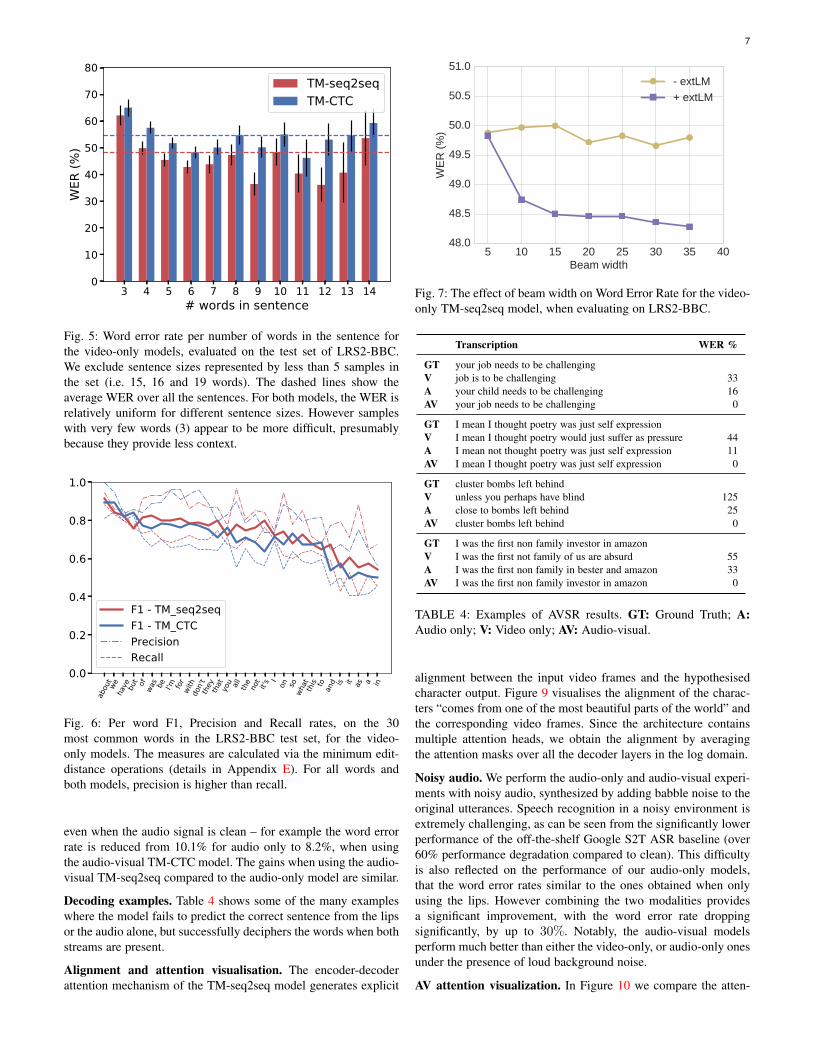
In Figure 5 we show how the WER changes as a functionof the number of words in a test sentence. Figure 6 showsthe performance of the models on the 30 most common words.Figure 7 shows the effect of increasing the beam width for thevideo-only TM-seq2seq model when evaluating on LRS2-BBC. Itis noteworthy that increasing the beam width is more beneficialwhen decoding with the external language model (+ extLM).

Decoding examples. The model learns to correctly predict com-plex unseen sentences from a wide range of content – examplesare shown in Table 3.

but this particular reality was not inevitable

it would have been completely alien to the rest of london

comes from one of the most beautiful parts of the world

everyone has gone home happy and that’s what it’s all about

especially when it comes to climate change

but it’s a different type of animal I want to show you right now

but these are one of the most wary birds in the world

there’s always historical treasures to look at

and so how does your brain give you that detail

but this is the source of innovation

the choices don’t make sense because it’s the wrong question

but it’s a global phenomenon

mortality is not going down it’s going up

TABLE 3: Examples of unseen sentences that TM-seq2seq cor-rectly predicts (video only).

6.2 Audio-visual speech recognitionThe visual information can be used to improve the performance ofASR, particularly in environments with background noise [36, 38,40]. Here, we analyse the performance of the audio-visual modelsdescribed in Section 3.

Results. The results in Table 2 demonstrate that the mouthmovements provide important cues in speech recognition whenthe audio signal is noisy; and give an improvement in performance

7

3 4 5 6 7 8 9 10 11 12 13 14# words in sentence

0

10

20

30

40

50

60

70

80W

ER (%

)TM-seq2seqTM-CTC

Fig. 5: Word error rate per number of words in the sentence forthe video-only models, evaluated on the test set of LRS2-BBC.We exclude sentence sizes represented by less than 5 samples inthe set (i.e. 15, 16 and 19 words). The dashed lines show theaverage WER over all the sentences. For both models, the WER isrelatively uniform for different sentence sizes. However sampleswith very few words (3) appear to be more difficult, presumablybecause they provide less context.

abou

twe

have bu

t ofwa

s be I'm for with

don't they that you all the

not

it'sI on so

what this to and is it as a in

0.0

0.2

0.4

0.6

0.8

1.0

F1 - TM_seq2seqF1 - TM_CTCPrecisionRecall

Fig. 6: Per word F1, Precision and Recall rates, on the 30most common words in the LRS2-BBC test set, for the video-only models. The measures are calculated via the minimum edit-distance operations (details in Appendix E). For all words andboth models, precision is higher than recall.

even when the audio signal is clean – for example the word errorrate is reduced from 10.1% for audio only to 8.2%, when usingthe audio-visual TM-CTC model. The gains when using the audio-visual TM-seq2seq compared to the audio-only model are similar.

Decoding examples. Table 4 shows some of the many exampleswhere the model fails to predict the correct sentence from the lipsor the audio alone, but successfully deciphers the words when bothstreams are present.

Alignment and attention visualisation. The encoder-decoderattention mechanism of the TM-seq2seq model generates explicit

5 10 15 20 25 30 35 40Beam width

48.0

48.5

49.0

49.5

50.0

50.5

51.0

WE

R (

%)

­ extLM+ extLM

Fig. 7: The effect of beam width on Word Error Rate for the video-only TM-seq2seq model, when evaluating on LRS2-BBC.

Transcription WER %

GT your job needs to be challengingV job is to be challenging 33A your child needs to be challenging 16AV your job needs to be challenging 0

GT I mean I thought poetry was just self expressionV I mean I thought poetry would just suffer as pressure 44A I mean not thought poetry was just self expression 11AV I mean I thought poetry was just self expression 0

GT cluster bombs left behindV unless you perhaps have blind 125A close to bombs left behind 25AV cluster bombs left behind 0

GT I was the first non family investor in amazonV I was the first not family of us are absurd 55A I was the first non family in bester and amazon 33AV I was the first non family investor in amazon 0

TABLE 4: Examples of AVSR results. GT: Ground Truth; A:Audio only; V: Video only; AV: Audio-visual.

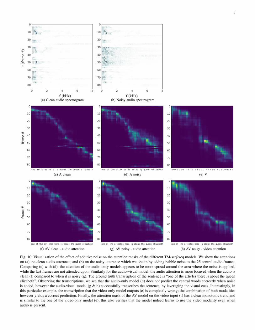
alignment between the input video frames and the hypothesisedcharacter output. Figure 9 visualises the alignment of the charac-ters “comes from one of the most beautiful parts of the world” andthe corresponding video frames. Since the architecture containsmultiple attention heads, we obtain the alignment by averagingthe attention masks over all the decoder layers in the log domain.

Noisy audio. We perform the audio-only and audio-visual experi-ments with noisy audio, synthesized by adding babble noise to theoriginal utterances. Speech recognition in a noisy environment isextremely challenging, as can be seen from the significantly lowerperformance of the off-the-shelf Google S2T ASR baseline (over60% performance degradation compared to clean). This difficultyis also reflected on the performance of our audio-only models,that the word error rates similar to the ones obtained when onlyusing the lips. However combining the two modalities providesa significant improvement, with the word error rate droppingsignificantly, by up to 30%. Notably, the audio-visual modelsperform much better than either the video-only, or audio-only onesunder the presence of loud background noise.

AV attention visualization. In Figure 10 we compare the atten-

8

tion masks of different TM-seq2seq models in the presence andabsence of additive babble noise in the audio stream.

6.3 Out-of-sync audio and videoHere, we assess the performance of the audio-visual models whenthe audio and video inputs are not temporally aligned. Sincethe audio and video have been synchronised in our dataset, wesynthetically shift the video frames to achieve an out-of-synceffect. We evaluate the performance on de-synchronised samplesof the LRS2-BBC dataset. We consider the TM-CTC and TM-seq2seq architectures, with and without fine-tuning on randomlyshifted samples. The results are shown in Figure 8. It is clear thatthe TM-seq2seq architecture is more resistant to these shifts. Weonly need to calibrate the model for one epoch for the out-of-sync effect to practically vanish. This showcases the advantageof employing independent encoder-decoder attention mechanismsfor the two modalities. In contrast, TM-CTC, that concatenates thetwo encodings, struggles to deal with the shifts, even after severalepochs of fine-tuning.

0 2 4 6 8 10 12Video offset (# frames)

7

8

9

10

11

12

13

14

15

WE

R (

%)

TM­seq2seqTM­seq2seq­finetunedTM­CTCTM­CTC­finetuned

Fig. 8: WER scored by the audio-visual models on LRS2-BBCwhen the video frames are artificially shifted by a number offrames compared to audio. The TM-seq2seq model is only fine-tuned for one epoch, while CTC for 4 epochs on the train-val set.

6.4 Discussion on seq2seq vs CTCThe TM-seq2seq model performs significantly better for lip-reading in terms of WER, when no audio is supplied. For audio-only or audio-visual tasks, the two methods perform similarly.However the CTC models appear to handle background noisebetter; in the presence of loud babble noise, both the audio-onlyand audio-visual TM-seq2seq models perform significantly worsethat their TM-CTC counterparts.

Training time. The TM-seq2seq models have a more complexarchitecture and are harder to train, with the full audio-visualmodel taking approximately 8 days to complete the full curriculumfor both datasets, on a single GeForce Titan X GPU with 12GBmemory. In contrast, the audiovisual TM-CTC model trains fasteri.e. in approximately 5 days on the same hardware. It should benoted however that since both architectures contain no recurrentmodules and no batch normalization, their implementation can beheavily parallelized into multiple GPUs.

comes f r om one o f t he mos t beau t i f u l pa r t s o f t he wo r l d

•••

vide

ofr

ame

#

transcription

Fig. 9: Alignment between the video frames and the characteroutput with TM-seq2seq. The alignment is produced by averagingall the encoder-decoder attention heads over all the decoder layersin the log domain.

Inference time. Decoding of the TM-CTC model does not requireauto-regression and therefore the CTC probabilities need only beevaluated once, regardless of the beam width W . This is not thecase for TM-seq2seq, where for every step of the beam search, thedecoder subnetwork needs to be evaluated W times. This makesthe decoding of the CTC model faster, which can be an importantfactor for deployment.

Language modelling. Both models perform better when an exter-nal language model is incorporated in the beam search, howeverthe gains are much higher for TM-CTC, since no explicit languageconsistency is enforced by the visual model alone.

Generalization to longer sequences. We observed that the TM-CTC model generalizes better and adapts faster as the sequencelengths are increased during the curriculum learning. We believethis also affects the training time as the latter takes more epochsto converge.

7 CONCLUSION

In this paper, we introduced a large-scale, unconstrained audio-visual dataset, LRS2-BBC, formed by collecting and preprocess-ing thousands of videos from the British television.

We considered two models that can transcribe audio and videosequences of speech into characters and showed that the samearchitectures can also be used when only one of the modalities ispresent. Our best visual-only model surpasses the performanceof the previous state-of-the-art on the LRS2-BBC lip readingdataset by a large margin, and sets a strong baseline for therecently released LRS3-TED. We finally demonstrate that visualinformation helps improve speech recognition performance evenwhen the clean audio signal is available. Especially in the presenceof noise in the audio, combining the two modalities leads to asignificant improvement.

9

0 2 4 6 8

0

10

20

30

40

50

60

70

80

t(fr

ame

#)

f (kHz)(a) Clean audio spectrogram

0 2 4 6 8

0

10

20

30

40

50

60

70

80

f (kHz)(b) Noisy audio spectrogram

fram

e#

the ar t i c l es here i s about the queen e l i zabeth

0

10

20

30

40

50

60

70

80

(c) A cleanone o f the ar t i c l es i s ac tua l l y queen e l i zabeth

0

10

20

30

40

50

60

70

80

(d) A noisyb e c a u s e i t ' s a b o u t t h r e e c u s t ome r s

0

10

20

30

40

50

60

70

80

(e) V

fram

e#

one of the ar t i c les here i s about the queen el i zabeth

0

10

20

30

40

50

60

70

80

(f) AV clean - audio attentionone of the ar t i c les here i s about the queen el i zabeth

0

10

20

30

40

50

60

70

80

(g) AV noisy - audio attentionone of the ar t i c les here i s about the queen el i zabeth

0

10

20

30

40

50

60

70

80

(h) AV noisy - video attention

Fig. 10: Visualization of the effect of additive noise on the attention masks of the different TM-seq2seq models. We show the attentionson (a) the clean audio utterance, and (b) on the noisy utterance which we obtain by adding babble noise to the 25 central audio frames.Comparing (c) with (d), the attention of the audio-only models appears to be more spread around the area where the noise is applied,while the last frames are not attended upon. Similarly for the audio-visual model, the audio attention is more focused when the audio isclean (f) compared to when it is noisy (g). The ground truth transcription of the sentence is “one of the articles there is about the queenelizabeth”. Observing the transcriptions, we see that the audio-only model (d) does not predict the central words correctly when noiseis added, however the audio-visual model (g & h) successfully transcribes the sentence, by leveraging the visual cues. Interestingly, inthis particular example, the transcription that the video-only model outputs (e) is completely wrong; the combination of both modalitieshowever yields a correct prediction. Finally, the attention mask of the AV model on the video input (f) has a clear monotonic trend andis similar to the one of the video-only model (e); this also verifies that the model indeed learns to use the video modality even whenaudio is present.

10

REFERENCES

[1] M. Abadi, A. Agarwal, P. Barham, E. Brevdo, Z. Chen,C. Citro, G. S. Corrado, A. Davis, J. Dean, M. Devin, et al.Tensorflow: Large-scale machine learning on heterogeneousdistributed systems. arXiv preprint arXiv:1603.04467, 2016.

[2] T. Afouras, J. S. Chung, and A. Zisserman. Deep lip reading:A comparison of models and an online application. InINTERSPEECH, 2018.

[3] T. Afouras, J. S. Chung, and A. Zisserman. LRS3-TED:a large-scale dataset for visual speech recognition. arXivpreprint arXiv:1809.00496, 2018.

[4] Y. M. Assael, B. Shillingford, S. Whiteson, and N. de Freitas.Lipnet: Sentence-level lipreading. arXiv:1611.01599, 2016.

[5] D. Bahdanau, K. Cho, and Y. Bengio. Neural machine trans-lation by jointly learning to align and translate. Proceedingsof the International Conference on Learning Representa-tions, 2015.

[6] S. Bai, J. Z. Kolter, and V. Koltun. An empirical evaluationof generic convolutional and recurrent networks for sequencemodeling. arXiv preprint arXiv:1803.01271, 2018.

[7] W. Chan, N. Jaitly, Q. V. Le, and O. Vinyals. Listen, attendand spell. arXiv preprint arXiv:1508.01211, 2015.

[8] C. Chiu, T. N. Sainath, Y. Wu, R. Prabhavalkar, P. Nguyen,Z. Chen, A. Kannan, R. J. Weiss, K. Rao, K. Gonina,N. Jaitly, B. Li, J. Chorowski, and M. Bacchiani. State-of-the-art speech recognition with sequence-to-sequence mod-els. CoRR, abs/1712.01769, 2017.

[9] K. Cho, B. Van Merrienboer, C. Gulcehre, D. Bahdanau,F. Bougares, H. Schwenk, and Y. Bengio. Learning phraserepresentations using rnn encoder-decoder for statistical ma-chine translation. In EMNLP, 2014.

[10] J. Chorowski, D. Bahdanau, K. Cho, and Y. Bengio. End-to-end continuous speech recognition using attention-basedrecurrent NN: first results. In NIPS 2014 Workshop on DeepLearning, 2014.

[11] J. K. Chorowski, D. Bahdanau, D. Serdyuk, K. Cho, andY. Bengio. Attention-based models for speech recognition. InAdvances in Neural Information Processing Systems, pages577–585, 2015.

[12] J. S. Chung, A. Senior, O. Vinyals, and A. Zisserman. Lipreading sentences in the wild. In Proceedings of the IEEEConference on Computer Vision and Pattern Recognition,2017.

[13] J. S. Chung and A. Zisserman. Lip reading in the wild. InProceedings of the Asian Conference on Computer Vision,2016.

[14] J. S. Chung and A. Zisserman. Out of time: automated lipsync in the wild. In Workshop on Multi-view Lip-reading,ACCV, 2016.

[15] J. S. Chung and A. Zisserman. Lip reading in profile.In Proceedings of the British Machine Vision Conference,2017.

[16] R. Collobert, C. Puhrsch, and G. Synnaeve. Wav2letter: Anend-to-end convnet-based speech recognition system. CoRR,abs/1609.03193, 2016.

[17] M. Cooke, J. Barker, S. Cunningham, and X. Shao. Anaudio-visual corpus for speech perception and automaticspeech recognition. The Journal of the Acoustical Societyof America, 120(5):2421–2424, 2006.

[18] A. Czyzewski, B. Kostek, P. Bratoszewski, J. Kotus, andM. Szykulski. An audio-visual corpus for multimodal auto-

matic speech recognition. Journal of Intelligent InformationSystems, pages 1–26, 2017.

[19] C. Feichtenhofer, A. Pinz, and A. Zisserman. Convolutionaltwo-stream network fusion for video action recognition. InProceedings of the IEEE Conference on Computer Visionand Pattern Recognition, 2016.

[20] G. Galatas, G. Potamianos, and F. Makedon. Audio-visualspeech recognition incorporating facial depth informationcaptured by the kinect. In Signal Processing Conference(EUSIPCO), 2012 Proceedings of the 20th European, pages2714–2717. IEEE, 2012.

[21] A. Graves. Sequence transduction with recurrent neuralnetworks. arXiv preprint arXiv:1211.3711, 2012.

[22] A. Graves, S. Fernandez, F. Gomez, and J. Schmidhu-ber. Connectionist temporal classification: Labelling unseg-mented sequence data with recurrent neural networks. InProceedings of the International Conference on MachineLearning, pages 369–376. ACM, 2006.

[23] A. Graves and N. Jaitly. Towards end-to-end speech recog-nition with recurrent neural networks. In Proceedings of theInternational Conference on Machine Learning, pages 1764–1772, 2014.

[24] K. He, X. Zhang, S. Ren, and J. Sun. Deep residual learningfor image recognition. arXiv preprint arXiv:1512.03385,2015.

[25] G. Hinton, L. Deng, D. Yu, G. Dahl, A.-R. Mohamed,N. Jaitly, A. Senior, V. Vanhoucke, P. Nguyen, B. Kingsbury,and T. Sainath. Deep neural networks for acoustic modelingin speech recognition. IEEE Signal Processing Magazine,29:82–97, November 2012.

[26] A. Kannan, Y. Wu, P. Nguyen, T. N. Sainath, Z. Chen, andR. Prabhavalkar. An analysis of incorporating an externallanguage model into a sequence-to-sequence model. arXivpreprint arXiv:1712.01996, 2017.

[27] D. E. King. Dlib-ml: A machine learning toolkit. The Journalof Machine Learning Research, 10:1755–1758, 2009.

[28] D. P. Kingma and J. Ba. ADAM: A method for stochasticoptimization. In Proceedings of the International Conferenceon Learning Representations, 2015.

[29] O. Koller, H. Ney, and R. Bowden. Deep learning of mouthshapes for sign language. In Proceedings of the IEEEConference on Computer Vision and Pattern Recognition,pages 85–91, 2015.

[30] A. Krizhevsky, I. Sutskever, and G. E. Hinton. ImageNetclassification with deep convolutional neural networks. InAdvances in Neural Information Processing Systems, pages1106–1114, 2012.

[31] R. Lienhart. Reliable transition detection in videos: A surveyand practitioner’s guide. International Journal of Image andGraphics, August 2001.

[32] V. Liptchinsky, G. Synnaeve, and R. Collobert. Letter-based speech recognition with gated convnets. CoRR,abs/1712.09444, 2017.

[33] W. Liu, D. Anguelov, D. Erhan, C. Szegedy, S. Reed, C.-Y.Fu, and A. C. Berg. SSD: Single shot multibox detector.In Proceedings of the European Conference on ComputerVision, pages 21–37. Springer, 2016.

[34] B. D. Lucas and T. Kanade. An iterative image registrationtechnique with an application to stereo vision. In Proc. of the7th International Joint Conference on Artificial Intelligence,pages 674–679, 1981.

[35] A. L. Maas, Z. Xie, D. Jurafsky, and A. Y. Ng. Lexicon-free

11

conversational speech recognition with neural networks. InProceedings the North American Chapter of the Associationfor Computational Linguistics (NAACL), 2015.

[36] Y. Mroueh, E. Marcheret, and V. Goel. Deep multimodallearning for audio-visual speech recognition. In 2015 IEEEInternational Conference on Acoustics, Speech and SignalProcessing (ICASSP), pages 2130–2134. IEEE, 2015.

[37] K. Noda, Y. Yamaguchi, K. Nakadai, H. G. Okuno, andT. Ogata. Lipreading using convolutional neural network.In INTERSPEECH, pages 1149–1153, 2014.

[38] K. Noda, Y. Yamaguchi, K. Nakadai, H. G. Okuno, andT. Ogata. Audio-visual speech recognition using deep learn-ing. Applied Intelligence, 42(4):722–737, 2015.

[39] S. Petridis and M. Pantic. Deep complementary bottleneckfeatures for visual speech recognition. ICASSP, pages 2304–2308, 2016.

[40] S. Petridis, T. Stafylakis, P. Ma, F. Cai, G. Tzimiropoulos,and M. Pantic. End-to-end audiovisual speech recognition.CoRR, abs/1802.06424, 2018.

[41] O. Russakovsky, J. Deng, H. Su, J. Krause, S. Satheesh,S. Ma, S. Huang, A. Karpathy, A. Khosla, M. Bernstein,A. Berg, and F. Li. Imagenet large scale visual recognitionchallenge. International Journal of Computer Vision, 2015.

[42] H. Sak, A. W. Senior, K. Rao, and F. Beaufays. Fast andaccurate recurrent neural network acoustic models for speechrecognition. In INTERSPEECH, 2015.

[43] B. Shillingford, Y. Assael, M. W. Hoffman, T. Paine,C. Hughes, U. Prabhu, H. Liao, H. Sak, K. Rao, L. Bennett,M. Mulville, B. Coppin, B. Laurie, A. Senior, and N. de Fre-itas. Large-Scale Visual Speech Recognition. arXiv preprintarXiv:1807.05162, 2018.

[44] K. Simonyan and A. Zisserman. Very deep convolutionalnetworks for large-scale image recognition. In InternationalConference on Learning Representations, 2015.

[45] T. Stafylakis and G. Tzimiropoulos. Combining residualnetworks with LSTMs for lipreading. In Interspeech, 2017.

[46] I. Sutskever, O. Vinyals, and Q. Le. Sequence to sequencelearning with neural networks. In Advances in neuralinformation processing systems, pages 3104–3112, 2014.

[47] C. Szegedy, W. Liu, Y. Jia, P. Sermanet, S. Reed,D. Anguelov, D. Erhan, V. Vanhoucke, and A. Rabinovich.Going deeper with convolutions. In Proceedings of the IEEEConference on Computer Vision and Pattern Recognition,2015.

[48] S. Tamura, H. Ninomiya, N. Kitaoka, S. Osuga, Y. Iribe,K. Takeda, and S. Hayamizu. Audio-visual speech recogni-tion using deep bottleneck features and high-performancelipreading. In 2015 Asia-Pacific Signal and InformationProcessing Association Annual Summit and Conference (AP-SIPA), pages 575–582. IEEE, 2015.

[49] A. Vaswani, N. Shazeer, N. Parmar, J. Uszkoreit, L. Jones,A. N. Gomez, L. Kaiser, and I. Polosukhin. Attention Is AllYou Need. In Advances in Neural Information ProcessingSystems, 2017.

[50] M. Wand, J. Koutn, and J. Schmidhuber. Lipreading withlong short-term memory. In 2016 IEEE International Confer-ence on Acoustics, Speech and Signal Processing (ICASSP),pages 6115–6119. IEEE, 2016.

[51] Y. Wang, X. Deng, S. Pu, and Z. Huang. Residual Convo-lutional CTC Networks for Automatic Speech Recognition.arXiv preprint arXiv:1702.07793, 2017.

[52] Y. Wu, M. Schuster, Z. Chen, Q. V. Le, M. Norouzi,

W. Macherey, M. Krikun, Y. Cao, Q. Gao, K. Macherey,J. Klingner, A. Shah, M. Johnson, X. Liu, L. Kaiser,S. Gouws, Y. Kato, T. Kudo, H. Kazawa, K. Stevens,G. Kurian, N. Patil, W. Wang, C. Young, J. Smith, J. Riesa,A. Rudnick, O. Vinyals, G. Corrado, M. Hughes, andJ. Dean. Google’s neural machine translation system: Bridg-ing the gap between human and machine translation. CoRR,abs/1609.08144, 2016.

[53] J. Yuan and M. Liberman. Speaker identification on thescotus corpus. Journal of the Acoustical Society of America,123(5):3878, 2008.

[54] N. Zeghidour, N. Usunier, I. Kokkinos, T. Schatz, G. Syn-naeve, and E. Dupoux. Learning filterbanks from raw speechfor phone recognition. CoRR, abs/1711.01161, 2017.

[55] Y. Zhang, M. Pezeshki, P. Brakel, S. Zhang, C. Laurent,Y. Bengio, and A. C. Courville. Towards end-to-end speechrecognition with deep convolutional neural networks. CoRR,abs/1701.02720, 2017.

[56] Z. Zhou, G. Zhao, X. Hong, and M. Pietikainen. A review ofrecent advances in visual speech decoding. Image and visioncomputing, 32(9):590–605, 2014.

12

APPENDIX AVISUAL FRONT-END ARCHITECTURE

The details of the spatio-temporal front-end are given in Table 5.

Layer Type Filters Output dimensions

Conv 3D 5× 7× 7, 64, /[1, 2, 2] T × H2 ×

W2 × 64

Max Pool 3D /[1, 2, 2] T × H4 ×

W4 × 64

Residual Conv 2D [3× 3, 64] ×2 /1 T × H4 ×

W4 × 64

Residual Conv 2D [3× 3, 64] ×2 /1 T × H4 ×

W4 × 64

Residual Conv 2D [3× 3, 128] ×2 /2 T × H8 ×

W8 × 128

Residual Conv 2D [3× 3, 128] ×2 /1 T × H8 ×

W8 × 128

Residual Conv 2D [3× 3, 256] ×2 /2 T × H16 ×

W16 × 256

Residual Conv 2D [3× 3, 256] ×2 /1 T × H16 ×

W16 × 256

Residual Conv 2D [3× 3, 512] ×2 /2 T × H32 ×

W32 × 512

Residual Conv 2D [3× 3, 512] ×2 /1 T × H32 ×

W32 × 512

TABLE 5: Architecture details for the spatio-temporal visualfront-end [45]. The strides for the residual 2D convolutional blocksapply to the first layer of the block only (i.e. the total down-sampling factor in the network is 32). A short cut connection isadded after every pair of 2D convolutions [24]. The 2D convolu-tions are applied separately on every time-frame.

APPENDIX BTRANSFORMER ARCHITECTURE DETAILS

The details of the building blocks used by our models are outlinedin Figure 11. The same multi-head attention block shown is usedfor both the self-attention and encoder-decoder attention layers ofthe models. A multi-head attention block, as described by Vaswaniet al. [49], receives a query (Q), a key (K) and a value (V ) tensoras inputs and produces h context vectors, one for every attentionhead i:

Atti(Q,K, V ) = softmax((W q

i QT )T (W k

i KT )√

dk)(W v

i VT )T

where Q, K , and V have size dmodel and dk = dmodelh is the size

of every attention head. The h context vectors are concatenatedand propagated through a feedforward block that consists of twolinear layers with ReLU non-linearities in between. For the self-attention layers it is always Q = K = V , while for the encoder-decoder attention of the TM-seq2seq model, K = V are theencoder outputs to be attended upon and Q is the decoder input,i.e. the network’s output at the previous decoding step for the firstlayer and the output of the previous decoder layer for the rest.We use the same architecture hyperparameters as the original basemodel of Vaswani et al. [49] with dmodel = 512 and h = 8attention heads everywhere. The sizes of the two linear layers inthe feedforward block are F1 = 2048, F2 = 512.

APPENDIX CSEQ2SEQ DECODING WITH EXTERNAL LANGUAGEMODEL

For decoding with the TM-seq2seq model, we use a left-to rightbeam search with width W as in [26, 52], with the hypotheses ybeing scored as follows:

score(x, y) =log p(y|x) + α log pLM (y)

LP (y)

Dot product attention

Q K V

Dot + Softmax

Dot product attention

Dot

Linear Linear Linear

Multi-head attention

Q K V

Concat

+

Layer Normalization

Linear F1 + ReLu

Linear F2 + ReLu

+

Layer Normalization

h parallel heads

Feed-forward

Fig. 11: Details of multi-head attention building blocks

where p(y|x) and pLM (y) are the probabilities obtained from thevisual and language models respectively and LP is a length nor-

malization factor LP(y) =(5+|y|

6

)β[52]. We did not experiment

with a coverage penalty. The best values for the hyperparameterswere determined via grid search on the validation set: for decodingwithout the external language model they were set to W = 6,α = 0.0, β = 0.6 and for decoding with the external languagemodel (+ extLM) to W = 35, α = 0.1 β = 0.7.

APPENDIX DCTC DECODING ALGORITHM WITH EXTERNAL LAN-GUAGE MODEL

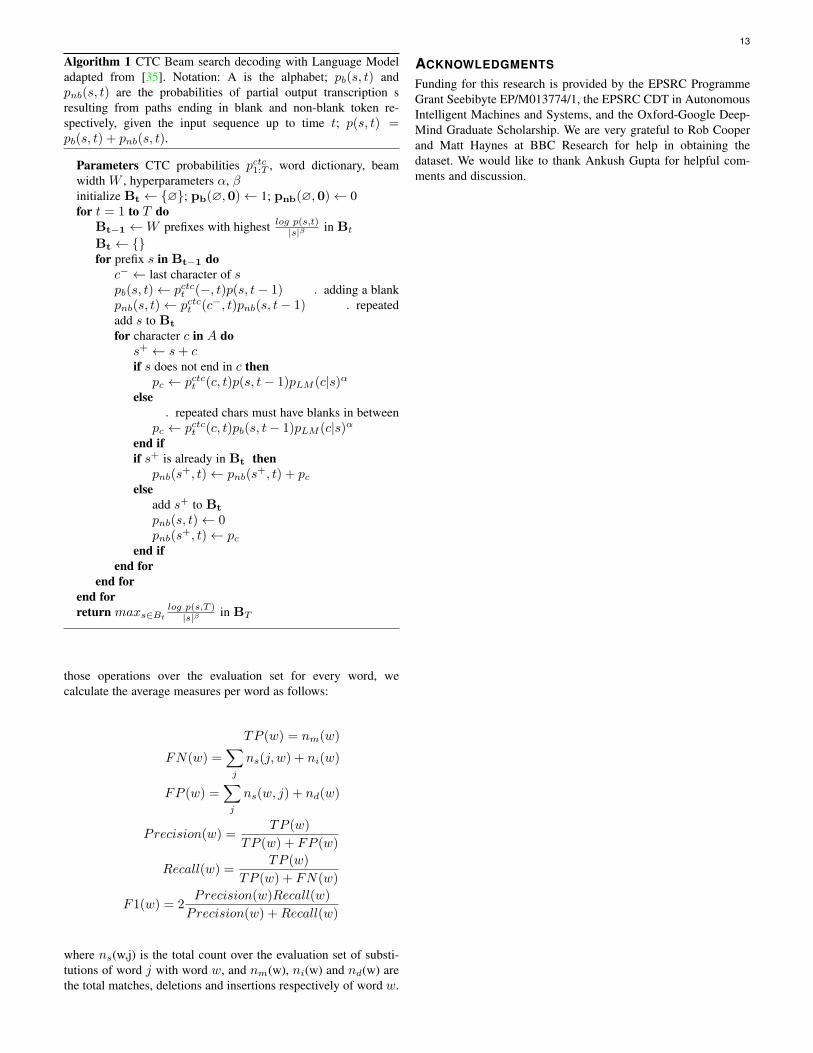
Algorithm 1 describes the CTC decoding procedure with anexternal language model. It is also a beam search with width Wand hyperparameters α and β that control the relative weight givento the LM and the length penalty. The beam search is similarto the one described for seq2seq above, with some additionalbookkeeping required to handle the emission of repeated and blankcharacters and normalization LP(y) = |y|β . We obtain the bestresults on the validation set with W = 100, α = 0.5, β = 0.1.

APPENDIX EPRECISION AND RECALL FROM EDIT DISTANCE

The F1, precision and recall rates shown in figure E, are calculatedfrom the word-wise minimum edit distance operations. For everysample in the evaluation set we can calculate the fewest wordsubstitution, insertion and deletion operations needed to get fromthe ground truth to the predicted transcription. After aggregating

13

Algorithm 1 CTC Beam search decoding with Language Modeladapted from [35]. Notation: A is the alphabet; pb(s, t) andpnb(s, t) are the probabilities of partial output transcription sresulting from paths ending in blank and non-blank token re-spectively, given the input sequence up to time t; p(s, t) =pb(s, t) + pnb(s, t).

Parameters CTC probabilities pctc1:T , word dictionary, beamwidth W , hyperparameters α, βinitialize Bt ← {∅}; pb(∅,0)← 1; pnb(∅,0)← 0for t = 1 to T do

Bt−1 ←W prefixes with highest log p(s,t)|s|β in Bt

Bt ← {}for prefix s in Bt−1 do

c− ← last character of spb(s, t)← pctct (−, t)p(s, t− 1) . adding a blankpnb(s, t)← pctct (c−, t)pnb(s, t− 1) . repeatedadd s to Bt

for character c in A dos+ ← s+ cif s does not end in c then

pc ← pctct (c, t)p(s, t− 1)pLM (c|s)αelse

. repeated chars must have blanks in betweenpc ← pctct (c, t)pb(s, t− 1)pLM (c|s)α

end ifif s+ is already in Bt then

pnb(s+, t)← pnb(s

+, t) + pcelse

add s+ to Bt

pnb(s, t)← 0pnb(s

+, t)← pcend if

end forend for

end forreturn maxs∈Bt

log p(s,T )|s|β in BT

those operations over the evaluation set for every word, wecalculate the average measures per word as follows:

TP (w) = nm(w)

FN(w) =∑j

ns(j, w) + ni(w)

FP (w) =∑j

ns(w, j) + nd(w)

Precision(w) =TP (w)

TP (w) + FP (w)

Recall(w) =TP (w)

TP (w) + FN(w)

F1(w) = 2Precision(w)Recall(w)

Precision(w) +Recall(w)

where ns(w,j) is the total count over the evaluation set of substi-tutions of word j with word w, and nm(w), ni(w) and nd(w) arethe total matches, deletions and insertions respectively of word w.

ACKNOWLEDGMENTS

Funding for this research is provided by the EPSRC ProgrammeGrant Seebibyte EP/M013774/1, the EPSRC CDT in AutonomousIntelligent Machines and Systems, and the Oxford-Google Deep-Mind Graduate Scholarship. We are very grateful to Rob Cooperand Matt Haynes at BBC Research for help in obtaining thedataset. We would like to thank Ankush Gupta for helpful com-ments and discussion.