1 CS 6910 – Pervasive Computing Spring 2007 Section 5 (Ch.5): Cellular Concept Prof. Leszek Lilien...

1

CS 6910 – Pervasive ComputingSpring 2007

Section 5 (Ch.5):

Cellular ConceptProf. Leszek Lilien

Department of Computer ScienceWestern Michigan University

Slides based on publisher’s slides for 1st and 2nd edition of: Introduction to Wireless and Mobile Systems by Agrawal & Zeng

© 2003, 2006, Dharma P. Agrawal and Qing-An Zeng. All rights reserved.

Some original slides were modified by L. Lilien, who strived to make such modifications clearly visible. Some slides were added by L. Lilien, and are © 2006-2007 by Leszek T. Lilien.

Requests to use L. Lilien’s slides for non-profit purposes will be gladly granted upon a written request.

Copyright © 2003, Dharma P. Agrawal and Qing-An Zeng. All rights reserved 2

Chapter 5

Cellular Concept


Outline Cell Shape

Actual cell/Ideal cell Signal Strength Handoff Region Cell Capacity

Traffic theory Erlang B and Erlang C

Cell Structure Frequency Reuse Reuse Distance Cochannel Interference Cell Splitting Cell Sectoring


5.1. Introduction Cell (formal def.)

= an area wherein the use of radio communication resources by the MS is controlled by a BS

Cell design is critical for cellular systems Size and shape dictate performance to a large extent

For given resource allocation and usage patterns

This section studies cell parameters and their impact

© 2007 by Leszek T. Lilien


5.2. Cell Area

Cell

R

(a) Ideal cell (b) Actual cell

R

R R

R

(c) Different cell models

[LTL] Cell size & shape are most important parameters in

cellular systems Informally, a cell is an area covered by a transmitting

station (BS) (with all MSs connected to and serviced by the BS) Recall:

Ideal cell shape (Fig. a) is circular Actual cell shapes (Fig. b) are caused by reflections & refractions

Also reflections & refractions from air particles Many cell models (Fig. c) approximate actual cell shape

Hexagonal cell model most popularSquare cell model second most popular

(Modified by LTL)


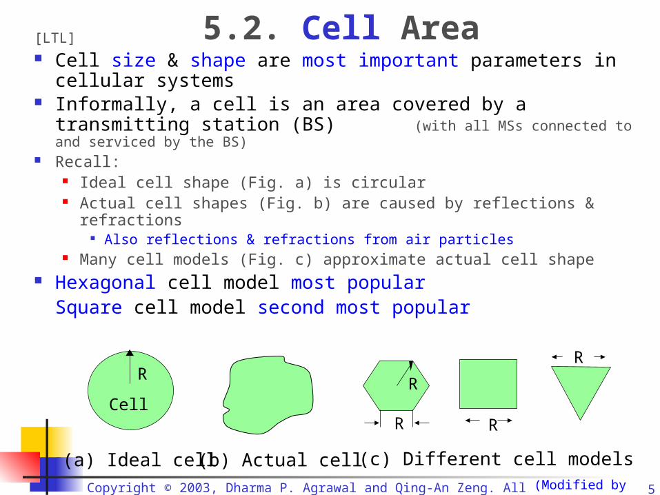
Impact of Cell Shape & Radius on Service Characteristics

Note: Only selected parameters from Table will be discussed (later) For given BS parameters, the simplest way of increase # of channels

available in an area, reduce cell size Smaller cells in a city than in a countryside

(Modified by LTL)


5.3. Signal Strength and Cell Parameters

[http://en.wikipedia.org/wiki/DBm] dBm (used in following slides) = an abbreviation for the

power ratio in decibel (dB) of the measured power referenced to 1 mW (milliwatt) dBm is an absolute unit measuring absolute power

Since it is referenced to 1 mW In contrast, dB is a dimensionless unit, which is used when

measuring the ratio between two values (such as signal-to-noise ratio)

Examples: 0 dBm = 1 mW 3 dBm ≈ 2 mW

Since a 3 dB increase represents roughly doubling the power −3 dBm ≈ 0.5 mW

Since a 3 dB decrease represents roughly cutting in half the power

… more examples – next slide …



5.3. Signal Strength and Cell Parameters – cont.

[http://en.wikipedia.org/wiki/DBm] Examples – cont.

60 dBm = 1,000,000 mW = 1,000 W = 1 kW Typical RF power inside a microwave oven

27 dBm = 500 mW Typical cellphone transmission power (some claim that users’ brains

are being fried) 20 dBm= 100 mW

Bluetooth Class 1 radio, 100 m range = max. output power from unlicensed FM transmitter (4 dBm = 2.5 mW - BT Class 2 radio, 10 m range)

−70 dBm = 100 pW (yes, “-”!!!) Average strength of wireless signal over a network See next slide!!! Average for the range: −60 to −80 dBm

−60 dBm= 1 nW = 1,000 pW −80 dBm= 10 pW



Signal Strength for Two Adjacent Cells with Ideal Cell Boundaries

Select cell i on left of boundary Select cell j on right of boundary

Cell i Cell j

-60

-70-80

-90

-100

-60-70

-80-90

-100

Signal strength (in dBm)

Recall:−70 dBm = 100 pW- average strength of wireless signal over a network

Ideal boundary


Signal Strength for Two Adjacent Cells with Actual Cell Boundaries

Signal strength contours indicating actual cell tiling. This happens because of terrain, presence of obstacles and signal attenuation in the atmosphere.

-100

-90-80

-70

-60

-60-70

-80

-90

-100

Signal strength (in dB)

Cell i Cell j

Recall:−70 dBm = 100 pW- average strength of wireless signal over a network


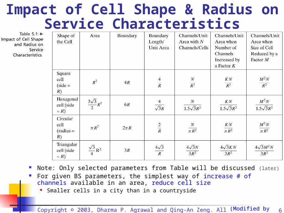
Power of Single Received Signal as Function of Distance from Single

BS

Next slide:Situation for signal power received from 2 BSs


Powers of Two Received Signals as Functions of Distances from Two

BSs

BSi

Sig

nal s

tren

gth

due

to B

Sj

X1

Sig

nal s

tren

gth

due

to B

Si

BSjX3 X4 X2X5

MS

Pmin

Pi(x) Pj(x)

Observe: Pj(X1) ≈ 0 Pi(X2) ≈ 0 Pj(X3) > Pmin (of course, Pi(X3) >> Pj(X3) > Pmin)

Pi(X4) > Pmin (of course, Pj(X4) >> Pi(X4) > Pmin)

Pj(X5) = Pi(X5)(Modified by

LTL)


Received Signals and Handoff (=Handover)

If MS moves away from BSi and towards BSj (as

shown), hand over MS from BSi and to BSj between X3 & X4

MS (SUV in the Figure) can receive the following signals: At X < X3 - can receive signal only from BSi (since Pj(X) < Pmin) At X3 < X < X4 - can receive signals from both BSi & BSj

At X > X4 - can receive signal only from BSj (since Pi(X) < Pmin)

BSi

Sig

nal s

tren

gth

due

to B

Sj

X1

Sig

nal s

tren

gth

due

to B

Si

BSjX3 X4 X2X5

MS

Pmin

Pi(x) Pj(x)

X

(Modified by LTL)


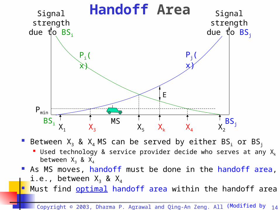
Handoff Area

BSi

Signal strength due to BSj

X1

Signal strength due to BSi

BSjX3 X4 X2X5

E

Xk

MS

Pmin

Pi(x) Pj(x)

Between X3 & X4 MS can be served by either BSi or BSj Used technology & service provider decide who serves at any Xk

between X3 & X4

As MS moves, handoff must be done in the handoff area, i.e., between X3 & X4

Must find optimal handoff area within the handoff area (Modified by

LTL)


Optimal Handoff Area &

Ping-pong Effect

BSi

Signal strength due to BSj

X1

Signal strength due to BSi

BSjX3 X4 X2X5

E

XkMS

Pmin

Pi(x) Pj(x)

Where is the optimum handoff area? Is it X5? - both signals have equal strength there

Ping-pong effect in handoff Imagine MS driving “across” X5 towards BSj, then turning

back and driving “across” X5 towards BSi, then turning back and driving “across” X5 towards BSj, then ….

Solution for avoiding ping-pong effect Maintain link with BSi up to point Xk where:

Pj(Xk) > Pj(Xk) + E (E - a chosen threshold)© 2007 by Leszek T. Lilien


Handoff in a Rectangular Cell Handoff affected by:

Cell area and shape MS mobility pattern

Different for each user & impossible to predict=> Can’t optimize handoff by matching cell shape to MS mobility

Illustration: How handoff related to mobility & rectangular cell area

Derivation (next slides – skipped) Results: Intuitively handoff is minimized when:

Rectangular cell is aligned [=its sides are aligned] with vertical & horizontal axes

AND the ratio of the numbers N1 and N2 of MSs crossing cell sides R1

and R2 is inversely proportional to the ratio of the lengths of R1 and R2



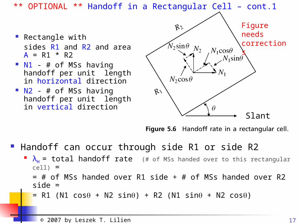
Rectangle withsides R1 and R2 and area A = R1 * R2

N1 - # of MSs having handoff per unit length in horizontal direction

N2 - # of MSs having handoff per unit length in vertical direction


Handoff can occur through side R1 or side R2 λH = total handoff rate (# of MSs handed over to this rectangular cell) =

= # of MSs handed over R1 side + # of MSs handed over R2 side == R1 (N1 cos + N2 sin) + R2 (N1 sin + N2 cos)

** OPTIONAL ** Handoff in a Rectangular Cell – cont.1

Figure needs corrections

Slant


How to minimize λH for a given

Assuming that A = R1 * R2 is constant, do:

Set R2 = A/ R1 Differentiate λH with respect to

R1 Equate it to zero

It gives (note: X1 = N1, X2 = X2):

Now, total handoff rate is:

H is minimized when =0, giving

Intuitively: Handoff is minimized when: “Rectangular cell is aligned [its sides are aligned] with vertical and

horizontal axes”AND the ratio of the number of MSs crossing cell sides R1 and R2 is

inversely proportional to the ratio of their lengths [TEXTBOOK: “the number of MSs crossing boundary is inversely proportional to the value of the other side of the cell”]

*** OPTIONAL *** Handoff in a Rectangular Cell – cont.2

sincos

cossin

21

212

1 XX

XXAR

cossin

sincos

21

2122 XX

XXAR

cossinsincos22121

XXXXAH

2

1

2

1212

X

X

R

RandXAXH

R2/R1 = N1/N2

Slant

Figure needs corrections


5.4. Cell Capacity Offered load

a = Twhere: - mean call arrival rate = avg. # of MSs requesting service per sec. T – mean call holding time = avg. length of call

ExampleOn average 30 calls generated per hour (3.600 sec.) in a cell

=> Arrival rate = 30/3600 calls/sec. = 0.0083333… calls/sec.


5.4. Cell Capacity – cont. 1

Erlang unit - a unit of telecommunications traffic (or

other traffic) [http://en.wikipedia.org/wiki/Erlang_unit]

http://en.wikipedia.org/wiki/Erlang: Agner Krarup Erlang (1878–1929) the Danish mathematician, statistician, and engineer after

whom the Erlang unit was named Erlang Shen is a famous Chinese deity

1 Erlang: 1 channel being in continuous (100%) useOR 2 channels being at 50% use (2 * 1/2 Erlang = 1 Erlang )

OR 3 channels being at 33.333… % use (3 * 1/3 Erlang = 1 Erlang )

OR …

Example 1: An office with 2 telephone operators, both busy 100% of the time => 2 * 100% = 2 * 1.0 = 2 Erlangs of traffic



5.4. Cell Capacity – cont. 2

Example 2 (Erlang as "use multiplier" per unit time) [ibid] 1 channel being used:

100% use => 1 Erlang 150% use => 1.5 Erlang

E.g. if total cell phone use in a given area per hour is 90 minutes => 90min./60min = 1.5 Erlangs

200% use => 2 Erlangs E.g. if total cell phone use in a given area per hour is 120 minutes

Traffic a in Erlangsa [Erlang] = λ [calls/sec.] * T [sec./call]

Recall: λ - mean arrival rate, T -mean call holding time

Example: A cell with 30 requests generated per hour

=> λ = 30/3600 calls/sec. Avg. call holding time T = 6 min. /call = 360 sec./call

a = (30 calls / 3600 sec) * (360 sec/call) = 3 Erlangs

Modified by LTL

Erlangscall

Sec

Sec

Callsa 3

360

3600

30


** OPTIONAL ** Cell Capacity – cont.3

Avg. # of call arrivals during a time interval of length t: t

Assume Poisson distribution of service requestsThen Probability P(n, t) that n calls arrive in an interval of length t: t

n

en

ttnP

!),(

tetS 1)(

- the service rate (a.k.a. departure rate) - how many calls completed per unit time [calls/sec]

Then: Avg. # of call terminations during a time interval

of length t: t Probability that a given call requires service for time ≤ t:

Modified by LTL


Erlang B and Erlang C a – offerred traffic load

S - # of channels in a cell Erlang B formula = (mnemonics: “B” as “Blocking”)

Probability B(S, a) of an arriving call being blocked

,

!

1

!,

0

S

k

k

S

kaS

aaSB

,

!!1

!1,

1

0

S

i

iS

S

ia

aSSa

aSSa

aSC

Erlang C formula = (mnemonics: “C” closer to “d” in “delayed”)

Probability C(S, a) of an arriving call being delayed


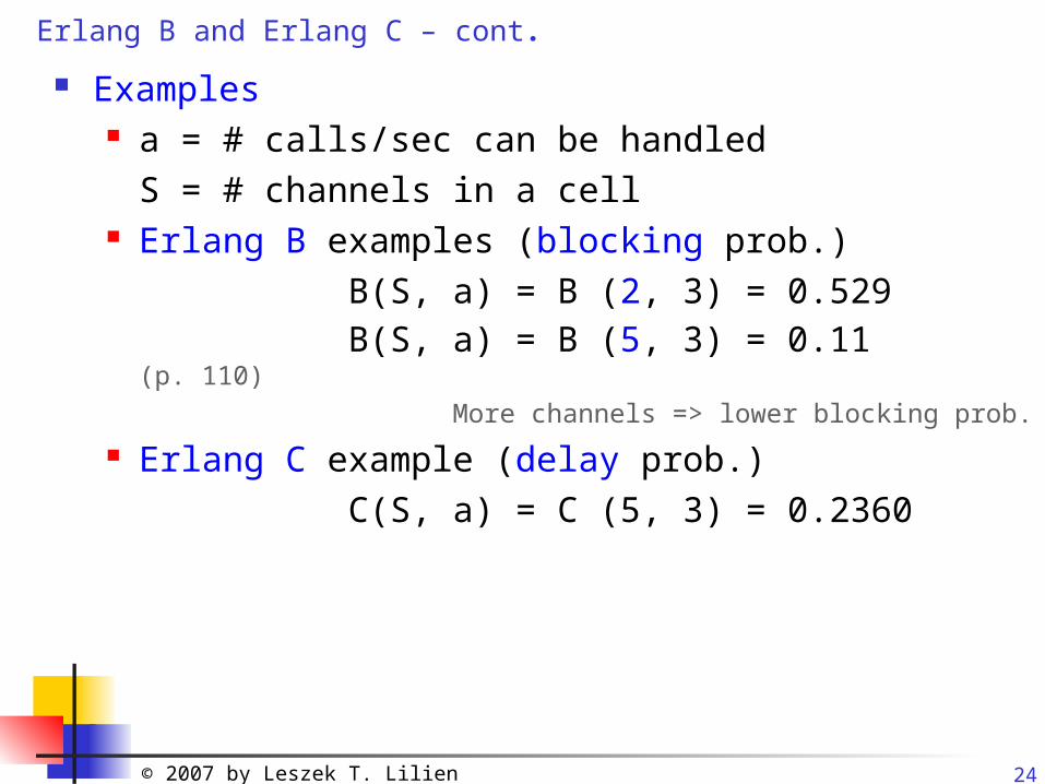
Erlang B and Erlang C – cont.

Examples a = # calls/sec can be handled

S = # channels in a cell Erlang B examples (blocking prob.)

B(S, a) = B (2, 3) = 0.529B(S, a) = B (5, 3) = 0.11 (p. 110)

More channels => lower blocking prob.

Erlang C example (delay prob.)C(S, a) = C (5, 3) = 0.2360



System Efficiency (Utilization) Efficiency = (Traffic_nonblocked) / (Total capacity) More precisely:

Efficiency =

= (offerred traffic load [Erlangs]) * (Pr. of call not being blocked) /

/ # of channels in the cell=

= a [Erlangs] * [1 – B(S, a)] / S

Example: Assume that: S= 2 channels in the cell, a = 3 calls/ sec => B (2, 3) = 0.529 - prob. of a call being blocked is 52.9

%

Efficiency = 3 [Erlangs] * [1 – B(2, 3)] / 2 = 3 [Erlangs] * (1 - 0.529) / 2 [channels] = 0.7065

= 70.65 %Modified by

LTL


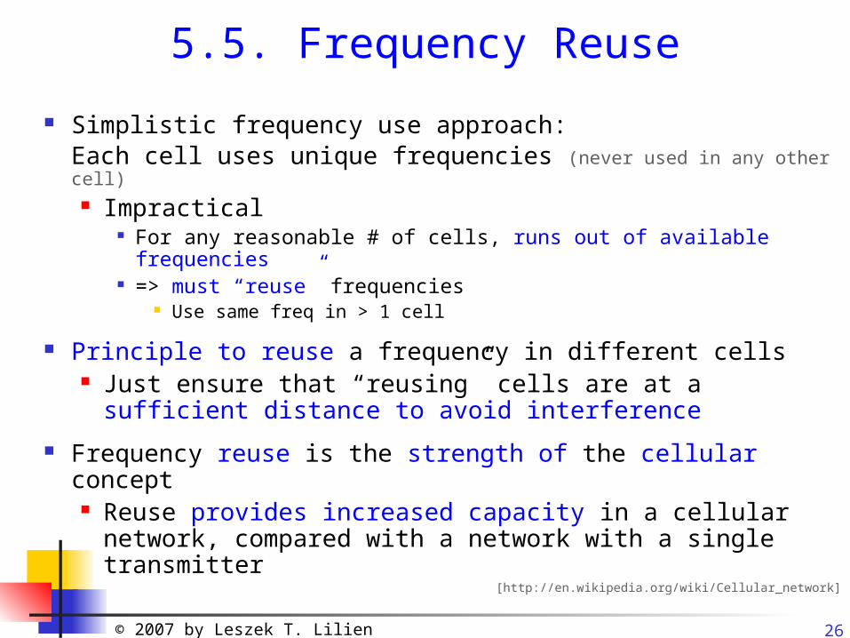
Simplistic frequency use approach:Each cell uses unique frequencies (never used in any other cell) Impractical

For any reasonable # of cells, runs out of available frequencies

=> must “reuse” frequencies Use same freq in > 1 cell

Principle to reuse a frequency in different cells Just ensure that “reusing” cells are at a sufficient

distance to avoid interference

Frequency reuse is the strength of the cellular concept Reuse provides increased capacity in a cellular

network, compared with a network with a single transmitter

[http://en.wikipedia.org/wiki/Cellular_network]


5.5. Frequency Reuse


Cell Structure

F2 F3F1F3

F2F1

F3

F2

F4

F1F1

F2

F3

F4F5

F6

F7

(a) Line Structure (b) Plan Structures

Frequency group = a set of frequencies used in a cell

Alternative cell structures: F1, F2, … - frequency groups Simplistic frequency assignments in figures

No reuse - unique frequency groups

Modified by LTL


Reuse Cluster

F1

F2

F3

F4F5

F6

F7 F1

F2

F3

F4F5

F6

F7

F1

F2

F3

F4F5

F6

F7 F1

F2

F3

F4F5

F6

F7

F1

F1

F1

F1

7-cell reuse cluster

F1, F2, … F7 - frequency groups

Cells form a cluster

E.g. 7-cell cluster of hexagonal cells

A reuse cluster Its structure &

its frequency groups are repeated to cover a broader service are

Modified by LTL


Reuse Distance• Reuse distance

• Between centers of cells reusing frequency groups

• For hexagonal cells, the reuse distance is given by

RND 3

where: R - cell radiusN - cluster size (# of cells per cluster)

=> need larger D for larger N or R

• Reuse factor is

q ~ D & q ~ 1/R & q ~ N(“~” means “is proportional”)

NR

Dq 3

F1

F2

F3

F4F5

F6

F7

F1

F2

F3

F4F5

F6

F7

F1

F1

Reuse distance D

R Cluster

Modified by LTL


Reuse Distance Again (a bigger picture)

F1

F2

F3

F4F5

F6

F7 F1

F2

F3

F4F5

F6

F7

F1

F2

F3

F4F5

F6

F7 F1

F2

F3

F4F5

F6

F7

F1

F1

F1

F1

7-cell reuse cluster

Reuse distance D

Modified by LTL


5.6. How to Form a Cluster The cluster size (# of cells per cluster):

N = i2 + ij + j2

where i and j are integers Substituting different values of i and j gives

N = 1, 3, 4, 7, 9, 12, 13, 16, 19, 21, 28, …

Most popular cluster sizes: N = 4 and N = 7

See next slide for hex clusters of different sizes

IMPORTANT (p.111/-1)

Unless otherwise specified, cluster size N = 7 assumed

Modified by LTL

Modified by LTL


Hex Clusters of Different SizesClusters designed for freq reuse


Finding Centers of All ClustersAround a Reference Cell

Finding centers of neighboring clusters (NCs) for hex cells

Procedure repeated 6 times (once for each side of a hex reference cell)

For each reference cell (RC), the six immediate NCs are:

right-toprightright-bottomleft-bottomleftleft-top

By finding centers of neighboring clusters (NCs), we simultaneously determine cells belonging to the current cluster



Neighboring Clusters for a Reference Cell


For the yellow RC, the followingNCs are shown:

Right Right-top Left-top

How to find namefor NC?

Draw a line fromthe center of RC tothe center of eachNC

We see lines for 3 NCsin the fig.

Thick red lines E.g., the cluster with green center cell is the “right”

neighborfor the cluster with the yellow center bec. Red line cuts the right edge of the yellow hexagon

F1

F2

F3

F4F5

F6

F7 F1

F2

F3

F4F5

F6

F7

F1

F2

F3

F4F5

F6

F7 F1

F2

F3

F4F5

F6

F7

F1

F1

F1

F1


For j = 1, the formula: N = i2 + ij + j2simplifies to: N = i2 + i + 1

j = 1 means that we travel only 1 step in the “60 degrees” direction (cf. Fig.)

N = 7 (selected) & j = 1 (fixed) => i =2 I.e., we travel exactly 2 steps to the right Fig. show i = 1, 2, 3, … but for N = 7 (and j = 1),

we have i = 2 only

Neighboring Clusters for a Reference Cell – cont. 1



[Repeated] N = 7 (selected) & j = 1 (fixed) => i =2 I.e., we travel only 2 steps to the right

ExampleTo get from the yellow cellto the green cell, we travel2 steps to the right(i = 2) & 1 step at60 degrees (j = 1)

Neighboring Clusters for a Reference Cell – cont. 2

F1

F2

F3

F4F5

F6

F7 F1

F2

F3

F4F5

F6

F7

F1

F2

F3

F4F5

F6

F7 F1

F2

F3

F4F5

F6

F7

F1

F1

F1

F1



Coordinate Plane & Labeling Cluster Cells

Step 1: Select a cell, its center becomes origin, form coordinate plane:u axis pointing to the right from the origin, and v axis at 60 degrees to u

Notice that “right” (= direction of u axis) is slanted to LHS All other directions are slanted analogously

Unit distance = dist.between centersof 2 adjacentcells

E.g., green cellidentifiedas (-3, 3)(-3 along u,3 along v)

E.g., red cellidentifiedas (4, -3)

Modified by LTL


Clusters formed using formula N = i2 + i + 1 Simplified from N = i2 + ij + j2 for j = 1

Cell label L For cluster size N and cell coordinates (u,v),

cell label L is:L = [(i+1) u + v] mod N

Examples (more in Table below) Cluster size N =7 => i = 2 (bec. N = i2 + i + 1) & L = (3u + v)

mod N (u,v) = (0, 0) => L = 0 mod 7 = 0 (u,v) = (-3, 3) => L = [(-9) + 3] mod 7 = (-6) mod 7 = 1 (u,v) = (4, -3) => L = [3 * 4 + (-3)] mod 7 = 9 mod 7 = 2© 2007 by Leszek T. Lilien

Coordinate Plane & Labeling Cluster Cells – cont. 1

Find 1 error in Table 5.2


Cell Labels for 7-Cell ClusterNote:Circles drawn to help finding clusters

Green and red dots indicate cells at(-3, 3) and(4, -3)

OBSERVE: Cells within each cluster are labeled in the same way!

Modified by LTL


Cell Labels for 13-Cell ClusterOBSERVE:

1) For 7-cell clusters, cells within clusters had labels 0-6

2) Here, for13-cell clusters, cells within clusters have labels 0-12

3) N = 13 & j = 1 => i = 3=> to get from (0,0) to the center of blue NC, go 3steps right, then 1 step at 60 degreesNote: “right” is slanted (bec. axis v is slanted)!

E.g., to get from (0,0) to its blue dot NC go 3 steps along u, then 1 step at 60 degrees

Modified by LTL


5.7. Cochannel Interference Slide 39: N = 7 => 6

NCs (neighboring clusters) with cells reusing each Fx of “our” cluster(Slide 40: N = 13 => 6 NCs w/ cells reusing each Fx)

BSs of NCs are called1st-tier cochannel BSs

Di ≥ D - R (cf. next slide)

BSs of “next ring” of neighbors are called2nd-tier cochannel BSs

At dist’s ≥ 2 * D (approx.)

Assuring reuse distance only limits interference

Does not eliminate it completely Observe that: (1) Di’s are not identical (D6 is the

smallest)(2) Di’s differ from reuse distance (< or >) Modified by

LTL

First-tiercochannel BS

MS

Serving BS

Second-tiercochannel BS

R

D1

D2

D3

D4

D5

D6

D

2D


Worst Case of Cochannel Interference

Worst case whenD1 = D2 ≈ D – RandD3 ≈ D6 = DandD4 ≈ D5 = D + R

Modified by LTL

MS

Serving BSCo-channel BS

R

D1

D2

D3

D4

D5

D6

R

D

D

D

D

D

D


Cochannel Interference

Cochannel interference ratio (CCIR)

M

kkI

C

ceInterferen

Carrier

I

C

1

where Ik is co-channel interference from BSk

M is the max. # of co-channel interfering cells

Example: N = 7 => M = 6

6

k

k

RD

C

I

C

1

where - propagation path loss slope( = from 2 to 5)


5.8. Cell Splitting

Medium cell(medium density)

Large cell (low density)

Small cell(high density)

Use largecell normally

When trafficload increases(e.g., increased #

of users in a cell),switch to medium-sized cells

Requires more BSs If increased again, switch to small cells

Requires even more BSs

Smaller xmitting power for smaller cells => reduced cochannel interference


5.9. Cell Sectoring (by Antenna Design) So far we assumed omnidirectional antennas

Propagate equal-strength signal in all directions (360 degrees)

Actually, antennas are directional Cover less than 360 degrees Most common: 120 / 90 / 60 degrees

Directional antennas are a.k.a. sectored antennasCells served by them known as sectored cells

To cover 360 degrees with directional antennas, need 3, 4 or 6 antennas

For 120- / 90- / 60- degree antennas, respectively Cf. next slide



5.9. Cell Sectoring (by Antenna Design) – cont.

60o

120o

(a). Omni (b). 120o sector

(e). 60o sector

120o

(c). 120o sector (alternate)

ab

c

ab

c

(d). 90o sector

90o

a

b

c

da

bc

d

ef

Above - sectoring of cells with directional antennas Together cover 360 degrees

Same effcect as a single omnidirectional antenna

Many antennas mounted on a single microwave tower E.g., for a BS in cell center: 3, 4, or 6 sectoral antennas on BS

tower

Modified by LTL


Cell Sectoring by Antenna Design –cont.

A

C

B

X

Advantages of sectoring Smaller xmission power

Each antenna covers smaller area Decreased cochannel interference

Since lower power Enhanced overall system’s spectrum efficiency

Placing directional antennas at corners Where three adjacent cells meet

E.g., BS tower X serves 120-degreeportions of cells A, B and C

Might seem that placement in corners requires 3 times more towers than placement with towers in centersActually, for a larger area, # of towers approx. the same (convince yourself)



Worst Case for Forward Channel Interference in Three-sector Cells

7.0qq

C

I

C

RDq /

BS1 – BS in our cell (e.g., in the cluster center, N = 7) BS2 & BS3 – are first-tier cochannel BSs = closest cells reusing our Fx (BS 1 in center => BS2, BS3 in centers of NCs)BS4 – not reusing => does not interfere

Distance from corresp. sector antennas of BS2/BS3 to MSD’ = D + 0.7 R (derivation - OPTIONAL - next slide & p. 118 )

© 2007 by Leszek T. Lilien CCIR (cochannel interf.

ratio):

Recall: - propagation path loss slope ( = 2 - 5)

RBS1

MS

R

D’

BS3

BS2

BS4

D

D


** OPTIONAL ** Derivation of D’ for Worst Case for Forward Channel Interference in Three-sector Cells – cont.

BS

MS

R

D’

D

BS

BS

BS

D


Worst Case for Forward Channel Interferencein Six-sector Cells

D +0.7R

MS

BS

BSR

Modified by LTL

RDq

q

C

I

C

/

7.0

CCIR (cochannel interf. ratio) for =4:

= 4 - propagation path loss slope

= (q + 0.7)41


The End of Section 5

1 CS 6910 – Pervasive Computing Spring 2007 Section 5 (Ch.5): Cellular Concept Prof. Leszek Lilien...

Documents

Transcript of 1 CS 6910 – Pervasive Computing Spring 2007 Section 5 (Ch.5): Cellular Concept Prof. Leszek Lilien...