1

Conclusion of Communication Optimizations

and start ofLoad Balancing Techniques

CS320

Spring 2003

Laxmikant Kale

http://charm.cs.uiuc.eduParallel Programming Laboratory

Dept. of Computer Science

University of Illinois at Urbana Champaign

2

Asynchronous reductions: Jacobi

• Convergence check– At the end of each Jacobi iteration, we do a convergence check

– Via a scalar Reduction (on maxError)

• But note: – each processor can maintain old data for one iteration

• So, use the result of the reduction one iteration later!– Deposit of reduction is separated from its result.

– MPI_Ireduce(..) returns a handle (like MPI_Irecv)

• And later, MPI_Wait(handle) will block when you need to.

3

Asynchronous reductions in Jacobi

compute compute

reduction

compute compute

reductionProcessor timeline

with sync. reduction

Processor timeline with async. reduction

This gap is avoided below

4

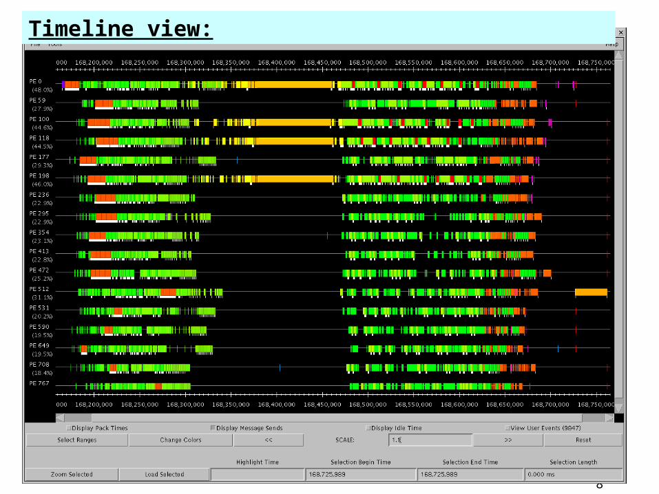
Performance tool snapshots

• From ab initio molecular dynamics application– (PPL in collaboration with Glenn Martyna and Mark Tuckerman)

5

Utilization Graph

6

Profile view: Processors on x-axis, stacked bar-chart of time spent for each

7

Overview: Processors on y-axis, time along x axis, white: busy, black: idle

8

Timeline view:

9

10

11

Load Balancing Techniques

CS320

Spring 2003

Laxmikant Kale

http://charm.cs.uiuc.eduParallel Programming Laboratory

Dept. of Computer Science

University of Illinois at Urbana Champaign

12

How to diagnose load imbalance?

• Often hidden in statements such as:– MPI_barrier is too slow

– MPI_reduce is too slow

– Very high synchronization overhead

• Most processors are waiting at a reduction

• Count total amount of computation (ops/flops) per processor– In each phase!

– Because the balance may change from phase to phase

13

Golden Rule of Load Balancing

Golden Rule: It is ok if a few processors idle, but avoid having processors that are overloaded with work

Finish time = max{Time on I’th processor}Excepting data dependence and communication overhead issues

Example: 50,000 tasks of equal size, 500 processors:

A: All processors get 99, except last 5 gets 100+99 = 199

OR, B: All processors have 101, except last 5 get 1

Fallacy: objective of load balancing is to minimize variance in load across processors

Identical variance, but situation A is much worse!

14

Amdahls’s Law and grainsize• Before we get to load balancing:• Original “law”:

– If a program has K % sequential section, then speedup is limited to 100/K.

• If the rest of the program is parallelized completely

• Grainsize corollary:– If any individual piece of work is > K time units, and the sequential

program takes Tseq , • Speedup is limited to Tseq / K

• So:– Examine performance data via histograms to find the sizes of remappable

work units– If some are too big, change the decomposition method to make smaller

units

15

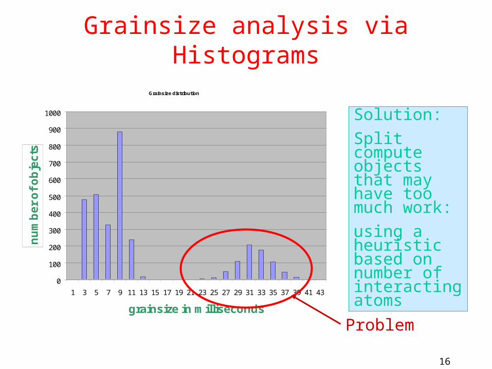
Grainsize Example: Molecular Dynamics

• In Molecular Dynamics Program NAMD:– While trying to scale it to 2000 processors

– Sequential step time was 57 seconds

– To run on 2000 processors, no object should be more than 28 msecs.

– Analysis using projections showed the following histogram:

16

Grainsize analysis via Histograms

Grainsize distribution

0

100

200

300

400

500

600

700

800

900

1000

1 3 5 7 9 11 13 15 17 19 21 23 25 27 29 31 33 35 37 39 41 43

grainsize in milliseconds

nu

mb

er

of

ob

jec

ts

Solution:

Split compute objects that may have too much work:

using a heuristic based on number of interacting atoms

Problem

17

Grainsize reduced

Grainsize distribution after splitting

0

200

400

600

800

1000

1200

1400

1600

1 3 5 7 9 11 13 15 17 19 21 23 25

grainsize in msecs

nu

mb

er o

f o

bje

cts

18

Grainsize: LeanMD for Blue Gene/L

• BG/L is a planned IBM machine with 128k processors• Here, we need even more objects:

– Generalize hybrid decomposition scheme

• 1-away to k-away 2-away :

cubes are half the size.

19

5000 vps

76,000 vps

256,000 vps

20

Load Balancing Strategies

• Classified by when it is done:– Initially

– Dynamic: Periodically

– Dynamic: Continuously

• Classified by whether decisions are taken with global information– Fully centralized

• Quite good a choice when load balancing period is high

– Fully distributed

• Each processor knows only about a constant number of neighbors

• Extreme case: totally local decision (send work to a random destination processor, with some probability).

– Use aggregated global information, and detailed neighborhood info.

21

Load Balancing: Unrestricted Exchange

• This is an initial OR periodic strategy

• Each processor reads (or has) Ni particles

• Before doing interesting things with the data, we want to distribute it equally across processors

• It doesn’t matter where each piece of data goes– No constraints

• Issues:– How to decide who sends data to whom

– How to minimize communication overhead in the process

22

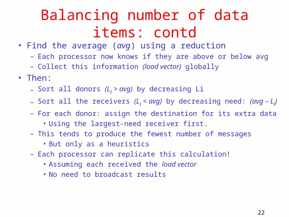
Balancing number of data items: contd

• Find the average (avg) using a reduction– Each processor now knows if they are above or below avg

– Collect this information (load vector) globally

• Then:– Sort all donors (Li > avg) by decreasing Li

– Sort all the receivers (Li < avg) by decreasing need: (avg – Li)

– For each donor: assign the destination for its extra data

• Using the largest-need receiver first.

– This tends to produce the fewest number of messages

• But only as a heuristics

– Each processor can replicate this calculation!

• Assuming each received the load vector

• No need to broadcast results

23

Balancing using Dimensional Exchange

• Log P phases: exchange info and then data with each neighbor– Send message saying how many items you have

– Compare your number with neighbor’s

• Calculate average

• Send overage to them

– Load is balanced at the end of log P phase

• In each phase, two halves are perfectly balanced

• After first phase, the two planes above are equally loaded– No need to return to exchanging data across planes (via red)

24

Dynamic Load Balancing Scenarios:

• Examples representing typical classes of situations– Particles distributed over simulation space

• Dynamic: because Particles move.

• Cases:– Highly non-uniform distribution (cosmology)

– Relatively Uniform distribution

– Structured grids, with dynamic refinements/coarsening

– Unstructured grids with dynamic refinements/coarsening

25

Example Case: Particles• Orthogonal Recursive Bisection (ORB)

– At each stage: divide Particles equally– Processor don’t need to be a power of 2:

• Divide in proportion – 2:3 with 5 processors

– How to choose the dimension along which to cut?• Choose the longest one

– How to draw the line?• All data on one processor? Sort along each dimension• Otherwise: run a distributed histogramming algorithm to find the

line, recursively– Find the entire tree, and then do all data movement at once

• Or do it in two-three steps.• But no reason to redistribute particles after drawing each line.

26

Particles: Oct/Quad Trees

• In ORB, each chunk has a brick shape, with non-square aspect ratio– Oct trees (Quad in 2D) lead to cubic boxes

• How to distribute particle-data into Oct trees?– Assume data is distributed (randomly)– Build a small top level tree across processors

• 2 or 3 deep– Send particles to their box

• Let each box create children if it has more than a threshold number of particles and send particles to them.

• Continue recursively• Note the tree is non-uniform (unlike ORB)

27

Particles: Space-filling curves

• Sort all particles using a key that mixes x, y and z coordinates– So particles with similar values for most significant bits of X,Y,Z

coordinates are clustered together.

• Snip this linearized list into equal size chunks

• This is almost like an Oct-tree, – Except nearby boxes have been collected together, for load balance

– First 3k bits are identical: belong to the same oct-tree node at the k’th level.

• But:– Sorting is relatively expensive to do every time

– Partitions don’t have a regular shape

– Because the space-filling curve jumps around, no real guarantee of communication minimization

28

Particles: Virtualization• You can apply virtualization to all the above methods:

– It becomes a two level strategy– Particles are grouped into a large number of boxes

• Much more than P• Cubes (oct-tree) or bricks (ORB)

– The “system” maps these boxes to processors

• Advantages:– You can use higher tolerance for imbalance (both oct and orb) during tree

formation– Particles can migrate among existing boxes, and load balancing can be

done by just moving boxes across processor • With a lower load balancing overhead• Less frequently, you can re-form the tree, if needed

– You can also locally split and coarsen it

29

Structured and Unstructured Grids/Meshes

• Similar considerations apply to these– Libraries like Metis partition Unstructured Meshes– ORB, Spacefilling curves are options for structured grids

• Virtualization:– Again, virtualization helps by reducing the cost of load

balancing• Use any scheme to partition data into large number of

chunks• Use a dynamic load balancer to map chunks to procs

– It can also decide• If communication costs are significant or not, and • Tune itself to communication patterns better.

30

Dynamic Load Balancing using Objects

• Object based decomposition (I.e. virtualized decomposition) helps– Allows RTS to remap them to balance load

– But how does the RTS decide where to map objects?

– Just move objects away from overloaded processors to underloaded processors

Just??

31

Measurement Based Load Balancing

• Principle of persistence– Object communication patterns and computational loads

tend to persist over time– In spite of dynamic behavior

• Abrupt but infrequent changes• Slow and small changes

• Runtime instrumentation– Measures communication volume and computation time

• Measurement based load balancers– Use the instrumented data-base periodically to make new

decisions– Many alternative strategies can use the database

32

Periodic Load balancing Strategies

• Stop the computation?• Centralized strategies:

– Charm RTS collects data (on one processor) about:

• Computational Load and Communication for each pair

– If you are not using AMPI/Charm, you can do the same instrumentation and data collection

– Partition the graph of objects across processors

• Take communication into account– Pt-to-pt, as well as multicast over a subset

– As you map an object, add to the load on both sending and receiving processor

• The red communication is free, if it is a multicast.

33

Object partitioning strategies• You can use graph partitioners like METIS, K-R

– BUT: graphs are smaller, and optimization criteria are different

• Greedy strategies– If communication costs are low: use a simple greedy strategy

• Sort objects by decreasing load• Maintain processors in a heap (by assigned load)• In each step:

– assign the heaviest remaining object to the least loaded processor

– With small-to-moderate communication cost:• Same strategy, but add communication costs as you add an object to a

processor– Always add a refinement step at the end:

• Swap work from heaviest loaded processor to “some other processor”• Repeat a few times or until no improvement

34

Object partitioning strategies

• When communication cost is significant:– Still use greedy strategy, but:

• At each assignment step, choose between assigning O to least loaded processor and the processor that already has objects that communicate most with O.

– Based on the degree of difference in the two metrics

– Two-stage assignments:

» In early stages, consider communication costs as long as the processors are in the same (broad) load “class”,

» In later stages, decide based on load

• Branch-and-bound– Searches for optimal, but can be stopped after a fixed time

35

Crack Propagation

Decomposition into 16 chunks (left) and 128 chunks, 8 for each PE (right). The middle area contains cohesive elements. Both decompositions obtained using Metis. Pictures: S. Breitenfeld, and P. Geubelle

As computation progresses, crack propagates, and new elements are added, leading to more complex computations in some chunks

36

Load balancer in action

0

5

10

15

20

25

30

35

40

45

501 6 11 16 21 26 31 36 41 46 51 56 61 66 71 76 81 86 91

Iteration Number

Nu

mb

er

of

Ite

rati

on

s P

er

se

con

dAutomatic Load Balancing in Crack Propagation

1. ElementsAdded 3. Chunks

Migrated

2. Load Balancer Invoked

37

Distributed Load balancing

• Centralized strategies– Still ok for 3000 processors for NAMD

• Distributed balancing is needed when:– Number of processors is large and/or

– load variation is rapid

• Large machines: – Need to handle locality of communication

• Topology sensitive placement

– Need to work with scant global information

• Approximate or aggregated global information (average/max load)

• Incomplete global info (only “neighborhood”)

• Work diffusion strategies (1980’s work by author and others!)

– Achieving global effects by local action…

38

Building on Object-based Load Balancing

• Application induced load imbalances• Environment induced performance issues:

– Dealing with extraneous loads on shared machines– Vacating workstations– Heterogeneous clusters– Shrinking and expanding the set of processors allocated to

a job!

• Automatic checkpointing– Restart on a different number of processors

• Pre-fetch capability– Out of Core execution– Optimizing Cache performance

39

Electronic Structures using CP• Car-Parinello method• Based on pinyMD

– Glenn Martyna, Mark Tuckerman

• Data structures:– A bunch of states (say 128)– Represented as

• 3D arrays of coeffs in G-space, and

• also 3D arrays in real space– Real-space prob. density– S-matrix: one number for each

pair of states• For orthonormalization

– Nuclei

• Computationally– Transformation from g-space

to real-space

• Use multiple parallel 3D-FFT

– Sums up real-space densities

– Computes energies from density

– Computes forces

– Normalizes g-space wave function

40

One Iteration

41

42

Points of interest

• Parallelizing the 3d-fft – Optimization of computation

– Optimization of communication

• Normalization– Involves all-to-all communication

43

3D FFT

44

Optimizating FFT

• 128 parallel FFTs– Need to optimize

• The 3D-space is sparsely populated• Reduce the number of FFTs• Reduce the amount of data transported

– Use run-length encoding

– Communication library

45

Optimizations

But, is this the biggest problem we have?