1

CHAPTER 5

POROUS MEDIA

2

5.1 Examples of Conduction in Porous Media

porous ring

coolant

(a)

blade

coolant

(c)

componentelectronic

micro channels

coolant

(d)

coolant

porous material

(e)

Fig. 5.1

(b)

porous shield

coolant

3

5.2 Simplified Heat Transfer Model

• Assume:

5.2.1 Porosity

• Definition: Porosity

(a)ALV

V

V

volumetotal

volumeporeP f (5.1)

At any point the solid and liquid are at the same temperature

4

Fig. 5.2

area flow total fA

Model: Pores are straight channels

(a) and (b) into eq. (5.1)

or

LAV ff (b)

A

AP f (c)

PAA f (5.2)

and solid wall area s

A

APAs )1( (5.3)

• Assume: Porosity is constant

5

5.2.2 Governing Equation: Cartesian Coordinates

One-dimensional transient conduction

= surface areaA

= flow ratem

Fig. 5.3

0 x

q dx

m= porosityP

= energy generationq

• Assumptions:

(1) Constant porosity

(2) Constant flow rate

(3) Constant properties (solid and fluid)

6

(4) Solid and fluid at same temperature

(5) Negligible changes in kinetic and potential energy

• Conservation of energy for element dx

Use Fourier’s law

Subscripts: s = solid, f = fluid

EEEE outgin (d)

TcmxT

PAkxT

APkE pffsin

)1( (e)

• Define: Conductivity of the solid-fluid matrix ask

7

fs kPkPk )1( (5.4)

(e) becomes

Use (f) to formulate

Tcmx

TAkE pfin

(f)

)(2

2

dxx

TTcmdx

x

TAk

x

TAkE pfout

(g)

dxAqEg (h)

Rate of energy change within the element E

dxt

TPAcdx

t

TAPcE pffpss

)1( (i)

8

Define: Heat capacity of the solid-fluid matrix aspc

pffpssp cPcPc )1( (5.5)

(i) becomes

(f), (g), (h) and (j) into (d)

dxt

TAcE p

(j)

t

T

k

q

x

T

kA

cm

x

T pf

1

2

2 (5.6)

= thermal diffusivity of solid-fluid matrix, defined as

pc

k

(5.7)

9

5.2.3 Boundary Conditions

(i) Specified temperature

Fig. 5.4

0

wallporous

reservoir x

m

oT (0)Tm T

h

1),0( TtT or 2),( TtLT (5.8)

At inlet or outlet

10

(ii) Convection at outlet boundary

Fig. 5.40

wallporous

reservoir x

m

oT (0)Tm T

h

TtLTh

x

tLTks ),(

),( (5.9)

(iii) Inlet supply reservoir: Conservation of energy for the control volume shown

x

tTAktTTcm opf

),0(),0( (5.10)

11

5.2.4 Cylindrical Systems

Conservation of energy and Fourier’s conduction lawapplied to the element dr:

m

rdr

Fig. 5.5

tT

kq

rT

rLk

cm

r

T pf

11

21 )(

2

2 (5.10)

12

5.3 Applications

Example 5.1: Steady State Conduction in a Porous Plate

Plate thickness = L

Solution(1) Observations • 1-D conduction in porous plate

Heated at x = L by convection: h, TCoolant reservoir temperature = oT

Design hot side temperature = dT

Determine: Am /

• dTLT )(

Fig. 5.40

wallporous

reservoir x

moT (0)Tm T

h

13

• depends on)(xT m

(2) Origin and Coordinates

See Fig. 5.4.

(3) Formulation (i) Assumptions

(1) Solid and fluid at same temperature

(2) Constant porosity

(3) Constant properties

(4) Constant flow rate

(5) No energy generation

(6) Steady state

14

(ii) Governing Equation

Eq. (5.6):

or

02

2

xd

dT

Lxd

Td (a)

is coolant flow parameter defined as

02

2

xd

dT

kA

cm

xd

Td pf

kA

Lcm pf (b)

15

(iii) Boundary Conditions

xd

dTTT

L o)0(

)0(

(c)

Convection at eq. (5.9),Lx

])([)(

TLThxd

LdTks (d)

sk = conductivity of the solid material

Supply reservoir, eq. (5.10), use definition of

Fig. 5.40

wallporous

reservoir x

moT (0)Tm T

h

16

(4) Solution Integrate (a) twice

Substitute into (e), introduce the Biot number

21 )/exp()( CLxL

CxT (e)

and (f) hLkL

TTC

s

o

/)/1(

)exp()(1

oTC 2

(g) 1)/(exp)(

Lx

Bi

Bi

TT

TxT

o

o

BC (c) and (d) give and 2C1C

17

sk

hLBi (h)

Determine required for : set x = L and in (g)

m dTT dTT

Bi

Bi

TT

TT

o

od

Solve for , use definitions of and Bi

)(

)(

odpf

d

s TTc

TTh

k

k

A

m

(i)

18

Dimensional check

Limiting check:

(5) Checking

(i) If h = 0 becomes insulated, entire Setting in (g) gives

),0( Bi Lx plate is at .oT 0Bi .)(

oTxT

should be at Settingand in (g) gives

(ii) If h ),( Bi )(LT .TBi Lx .)( TLT

entire plate is at Setting (iii) If m ),( .oT in (g) gives .)(

oTxT

BC (c) shows plate is insulated at entire plate at Setting in (g) gives

(iv) If 0m ),0( ,0x .T 0

.)( TxT

19

(6) Commentsm (i) Solution (g) shows that increasing lowers T)(

(ii) Solution depends on two parameters, andBi

(iii) Alternate solution for the required flow rate: Conservation of energy for a control volume from supply reservoir and :Lx

))(1(

)(

TTPhAdx

LdTPAkTcmTcm

d

fdpfopf

Use (d) to eliminate and rearrangedxLdT /)(

20

or)()1(

)()(

d

ds

fodpf

TTAPh

TTk

hPAkTTcm

)(

)]()/()1[(

odpf

dsf

TTc

TTPkkPh

A

m

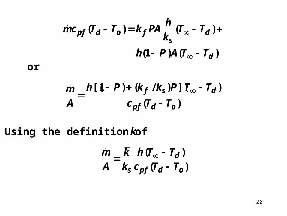
Using the definition of k

)(

)(

odpf

d

s TTc

TTh

k

k

A

m

21

Example 5.2:Transient Conduction in a Porous Plate

Plate thickness = L L

Am/

x

1T

Determine: Transient temperature

Reservoir temperature = oT

Initial temperature = oT

(1) Observations• One-D transient, porous plate

• At steady state 1),( TxT

Sudden change in surface temperatureto T1

22

(2) Origin and Coordinates

(3) Formulation (i) Assumptions

(1) Solid and fluid at same temperatures

(2) Constant porosity

(3) Constant properties

(4) Constant flow rate

(5) No energy generation

(6) Initially flow is established, plate temperature

= oT

23

(ii) Governing Equation

(iii) Boundary and Initial Conditions

t

T

k

q

x

T

kA

cm

x

T pf

1

2

2 (5.6)

L

Am/

x

1T

(1) 1),0( TtT

(2) 0),(

x

tLT

(3) oTxT )0,(

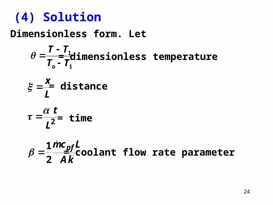
24

(4) SolutionDimensionless form. Let

= dimensionless temperature1

1

TT

TT

o

= distanceL

x

= time2L

t

= coolant flow rate parameterkA

Lcm pf2

1

25

Governing equation and boundary and initial conditionsbecome

Assume a product solution to (a)

xx2

2

2

(a)

(1) 0),0(

(2) 0),1(

(3) 1)0,(

)()(),( X (b)

26

(b) into (a), separate variables

02 22

2

nnnn X

d

dX

d

Xd

(c)

02 nnn

d

d

(d)

Solution to (c) depends on and . Only

gives characteristic values. Thus solution is given by

equation (A-6a)

2 2n 22

n

nnnnn MBMAX cossin)exp( (e)

and are constant, is defined asnA nB nM

22 nnM (f)

27

The solution to (d) is

)exp( 2 nnC (g)

is constant. BC (1) givesnC

0nB (h)

B.C. (2) gives the characteristic equation

(e) and (g) into (b)

BiMM nn tan (i)

1

2 sin)exp(),(n

nnn Ma (j)

28

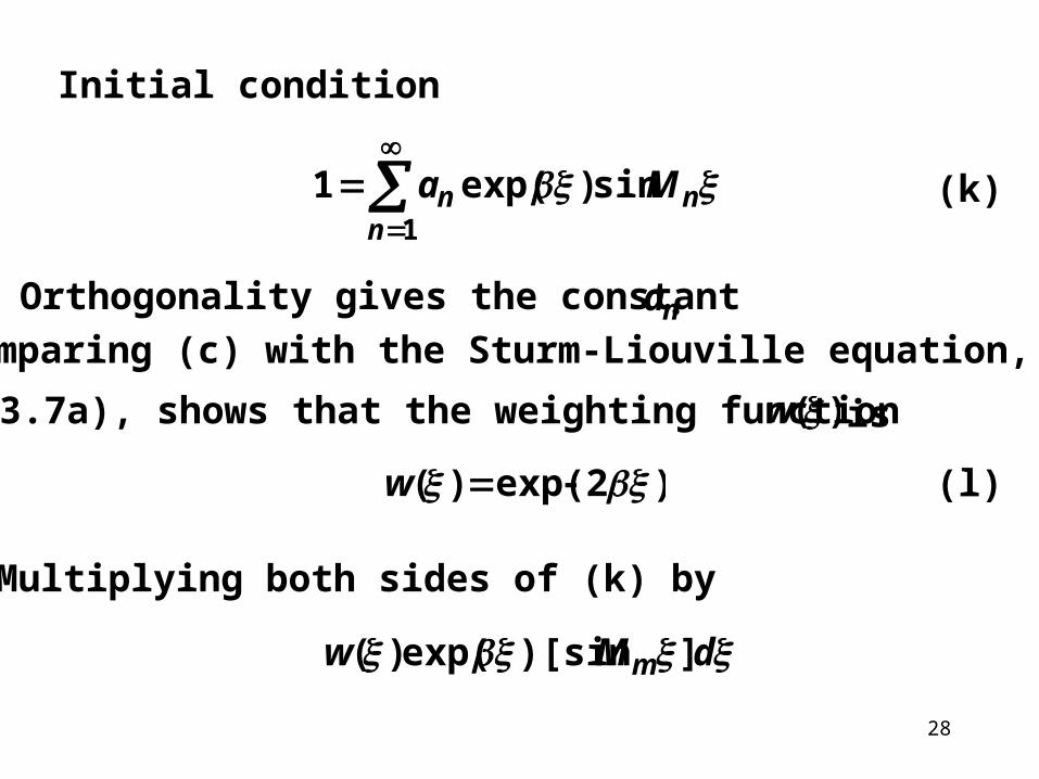
Initial condition

1

sin)exp(1n

nn Ma (k)

Orthogonality gives the constant . na

)2exp()( w (l)

Multiplying both sides of (k) by

dMw m ])[sinexp()(

is(3.7a), shows that the weighting function )(w

Comparing (c) with the Sturm-Liouville equation, eq.

29

Integrate from to and apply orthogonality,

eq. (3.9),

0 1

1

0

1

0])[sinexp(])[sinexp( dMadM nnn

Evaluate the integrals and solve for na

)2sin2)((

422

nnn

nn

MMM

Ma

(m)

(5) Checking

Dimensional check

Limiting check:

30

(6) Comments

In applications where coolant weight is an important design factor, weight requirement as determined by a transient solution is less than that given by a steady statesolution.The saving in weight depends on the length of the protection period.

At , entire plate at . Setting in (j) gives

, or .

t 1T 0),( 1),( TxT