1. Boolean Retrieval Definition: Information retrieval (IR) is finding material (usually documents) of an unstructured nature (usually text) that satisfies an information need from within large collection (usually on computer server or on the internet. DB-retrieval: “I’m sorry, I can only look up your order, if you give me your OrderId”. DB: strongly structured Reality: almost no data is truly „unstructured“ Given: Sheakespeare’s Collected Works Query: Brutus AND Caesar AND NOT Calpurinia Find the answer by grepping (UNIX –command all rows with a property) all the works of Shakespeare

Anthony and

Cleopatra

Julius Caesar

The Tempest (Sturm)

Hamlet Othello Macbeth ...

Anthony 1 1 0 0 0 1 Brutus 1 1 0 1 0 0 Caesar 1 1 0 1 1 1

Calpurnia 0 1 0 0 0 0 Cleopatra 1 0 0 0 0 0

mercy 1 0 1 1 1 1 worser

(Schlechtere) 1 0 1 1 1 0

(i,j)=1, if the play in column j contains the word of row i, 0 otherwise Answer of the Query: 110100 AND 110111 AND 101111 = 100100 „Anthony and Cleopatra“ and „Hamlet“ general example:

• 1 million documents • each document 1000 words (3 book pages) • 6 bytes per word

document collection=6 Gbyte typically: 500 000 distinct terms (words)

500 000 * 1 million = 0.5 Terabits(60 Gbyte) A system cannot handle this amount of data; Critical observation: the matrix is extremly sparse: 99.8% of cells are 0

1

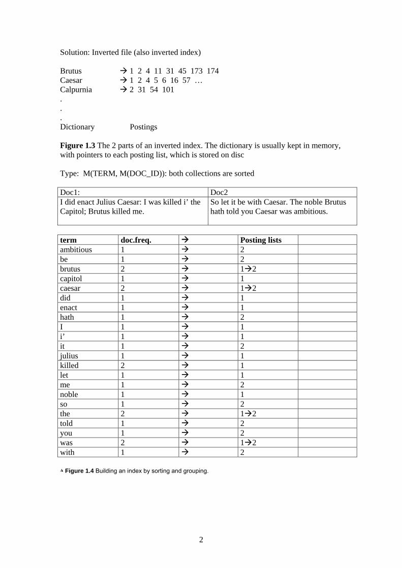
Solution: Inverted file (also inverted index) Brutus 1 2 4 11 31 45 173 174 Caesar 1 2 4 5 6 16 57 … Calpurnia 2 31 54 101 . . . Dictionary Postings Figure 1.3 The 2 parts of an inverted index. The dictionary is usually kept in memory, with pointers to each posting list, which is stored on disc Type: M(TERM, M(DOC_ID)): both collections are sorted Doc1: Doc2 I did enact Julius Caesar: I was killed i’ the Capitol; Brutus killed me.

So let it be with Caesar. The noble Brutus hath told you Caesar was ambitious.

term doc.freq. Posting lists ambitious 1 2 be 1 2 brutus 2 1 2 capitol 1 1 caesar 2 1 2 did 1 1 enact 1 1 hath 1 2 I 1 1 i’ 1 1 it 1 2 julius 1 1 killed 2 1 let 1 1 me 1 2 noble 1 1 so 1 2 the 2 1 2 told 1 2 you 1 2 was 2 1 2 with 1 2 ◮ Figure 1.4 Building an index by sorting and grouping.

2

INTERSECT(p1, p2) 1 answer ← [ ] 2 while p1 != NIL and p2 != NIL

3 do if docID(p1) = docID(p2) 4 then ADD(answer, docID(p1)) 5 p1 ← next(p1)

6 p2 ← next(p2) 7 else if docID(p1) < docID(p2) 8 then p1 ← next(p1)

9 else p2 ← next(p2) 10 return answer

◮ Figure 1.6 Algorithm for the intersection of two postings lists p1 and p2. Time: O(x+y);

x: number of entries of the first posting list y: number of entries of the second posting list

O(number_of_documents): A more general query needs query optimization (1.3) Brutus AND Caesar AND Calpurnia

Brutus 1 2 4 11 31 45 173 174 Caesar 1 2 4 5 6 16 57 … Calpurnia 2 31 54 101

(Calpurnia AND Brutus) AND Caesar This is a first justification for keeping the frequency of terms in the dictionary. (1.5) (madding OR crowd) AND (ignoble OR strife) AND (killed OR slain) mad: irr; ignoble: gemein; strife: Kampf; slain: getötet As before, we will get the frequencies for all terms, and we can then (conservatively) estimate the size of each OR by the sum of the frequencies of its disjuncts. We can then process the query in increasing order of the size of each disjunctive term. For arbitrary Boolean queries, we have to evaluate and temporarily store the answers for intermediate expressions in a complex expression. However, in many circumstances, either because of the nature of the query language, or just because this is the most common type of query that users submit, a query is purely conjunctive. tokenization: Input: Friends, Romans, Countrymen, lend me your ears; Output: Friends Romans Countrymen lend me your ears These tokens are often loosely referred to as terms or words.

3

2.3 Faster postings list intersection via skip pointers If the list lengths are m and n, the intersection takes O(m + n) operations. Can we do better than this? That is, empirically, can we usually process postings list intersection in sublinear time? We can, if the index isn’t changing too fast.

Figure 2.9 Postings lists with skip pointers. The postings intersection can use a skip pointer when the end point is still less than the item on the other list. One way to do this is to use a skip list by augmenting postings lists with skip pointers (at indexing time), as shown in Figure 2.9. Skip pointers are effectively shortcuts that allow us to avoid processing parts of the postings list that will not figure in the search results. The two questions are then where to place skip pointers and how to do efficient merging using skip pointers. Consider first efficient merging, with Figure 2.9 as an example. Suppose we’ve stepped through the lists in the figure until we have matched 8 on each list and moved it to the results list. We advance both pointers, giving us 16 on the upper list and 41 on the lower list. The smallest item is then the element 16 on the top list. Rather than simply advancing the upper pointer, we first check the skip list pointer and note that 28 is also less than 41. Hence we can follow the skip list pointer, and then we advance the upper pointer to 28 . We thus avoid stepping to 19 and 23 on the upper list.

4

INTERSECTWITHSKIPS(p1, p2) 1 answer ← [ ] 2 while p1 != NIL and p2 != NIL

3 do if docID(p1) = docID(p2) 4 then ADD(answer, docID(p1)) 5 p1 ← next(p1)

6 p2 ← next(p2) 7 else if docID(p1) < docID(p2) 8 then if hasSkip(p1) and (docID(skip(p1)) ≤ docID(p2))

9 then while hasSkip(p1) and (docID(skip(p1)) ≤ docID(p2))

10 do p1 ← skip(p1)

11 else p1 ← next(p1)

12 else if hasSkip(p2) and (docID(skip(p2)) ≤ docID(p1))

13 then while hasSkip(p2) and (docID(skip(p2)) ≤ docID(p1))

14 do p2 ← skip(p2)

15 else p2 ← next(p2) 16 return answer ◮ Figure 2.10 Postings lists intersection with skip pointers. 2.4 Positional postings and phrase queries Phrase: ”Stanford University“ is not intended to match the following sentence: The inventor Stanford Ovshinsky never went to university.

10% of web queries are phrase queries, and many more are implicit phrase queries (such as person names), entered without use of double quotes. A search engine should not only support phrase queries, but implement them efficiently. 2.4.1 Biword indexes The query

stanford university palo alto can be broken into the Boolean query on biwords:

“stanford university” AND “university palo” AND “palo alto”

Without examining the documents, we cannot verify that the documents matching the above Boolean query do actually contain the original 4 word phrase (false drop). BIWORD_INDEX_TYPE: M(TERM1, TERM2, M(DOC_ID)) An exhaustive biword dictionary greatly expands the size of the vocabulary. Single word queries like Stanford are hard to realize. A single word index is additionally needed. The concept of a biword index can be extended to longer sequences of words, and if the index includes variable length word sequences, it is generally referred to as a phrase index.

5

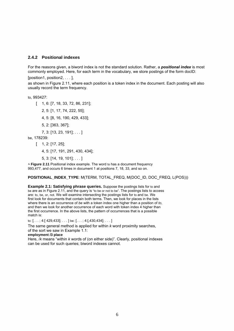
2.4.2 Positional indexes For the reasons given, a biword index is not the standard solution. Rather, a positional index is most commonly employed. Here, for each term in the vocabulary, we store postings of the form docID: [position1, position2, . . . ], as shown in Figure 2.11, where each position is a token index in the document. Each posting will also usually record the term frequency. to, 993427: [ 1, 6: [7, 18, 33, 72, 86, 231];

2, 5: [1, 17, 74, 222, 55]; 4, 5: [8, 16, 190, 429, 433]; 5, 2: [363, 367]; 7, 3: [13, 23, 191]; . . . ]

be, 178239: [ 1, 2: [17, 25];

4, 5: [17, 191, 291, 430, 434]; 5, 3: [14, 19, 101]; . . . ]

◮ Figure 2.11 Positional index example. The word to has a document frequency 993,477, and occurs 6 times in document 1 at positions 7, 18, 33, and so on. POSITIONAL_INDEX_TYPE: M(TERM, TOTAL_FREQ, M(DOC_ID, DOC_FREQ, L(POS))) Example 2.1: Satisfying phrase queries. Suppose the postings lists for to and be are as in Figure 2.11, and the query is “to be or not to be”. The postings lists to access are: to, be, or, not. We will examine intersecting the postings lists for to and be. We first look for documents that contain both terms. Then, we look for places in the lists where there is an occurrence of be with a token index one higher than a position of to, and then we look for another occurrence of each word with token index 4 higher than the first occurrence. In the above lists, the pattern of occurrences that is a possible match is: to: [. . . ; 4:[ 429,433]; . . . ] be: [. . . ; 4:[,430,434]; . . . ] The same general method is applied for within k word proximity searches, of the sort we saw in Example 1.1: employment /3 place Here, /k means “within k words of (on either side)”. Clearly, positional indexes can be used for such queries; biword indexes cannot.

6

POSITIONALINTERSECT(p1, p2, k) 1 answer ← [ ] 2 while p1 != NIL and p2 != NIL 3 do if docID(p1) = docID(p2) 4 then l ← [ ] 5 pp1 ← positions(p1)

6 pp2 ← positions(p2)

7 while pp1 != NIL

8 do while pp2 != NIL

9 do if |pos(pp1) − pos(pp2)| > k 10 then break 11 else ADD(l, pos(pp2)) 12 pp2 ← next(pp2)

13 while l != [ ] and |l[0] − pos(pp1)| > k 14 do DELETE(l[0]) 15 for each ps in l 16 do ADD(answer, [docID(p1), pos(pp1), ps]) 17 pp1 ← next(pp1)

18 p1 ← next(p1)

19 p2 ← next(p2) 20 else if docID(p1) < docID(p2) 21 then p1 ← next(p1)

22 else p2← next(p2)

23 return answer

◮ Figure 2.12 An algorithm for proximity intersection of postings lists p1 and p2. The algorithm finds places where the two terms appear within k words of each other and returns a list of triples giving docID and the term position in p1 and p2. Adding Britney Spears as a phrase index entry may only give a speedup factor to that query of about 3, since most documents that mention either word are valid results, whereas adding The Who as a phrase index entry may speed up that query by a factor of 1000.

7

3 Dictionaries and tolerant retrieval 3.1 Search structures for dictionaries

In the literature of data structures, the entries in the vocabulary (in our case, terms) are often referred to as keys.

2 Possibilities: hashing or search trees

The decisition depends on the following questions: (1) How many keys are we likely to have? (2) Is the number likely to remain static, or change a lot – and in the case of changes, are we likely to only have new keys inserted, or to also have some keys in the dictionary be del ted? e(3) What are the relative frequencies with which various keys will be accessed? Hashing has been used for dictionary lookup in some search engines. Each vocabulary term (key) is hashed into an integer over a large enough space that hash collisions are unlikely; collisions if any are resolved by auxiliary structures that can demand care to maintain. At query time, we hash each query term separately and following a pointer to the corresponding postings, taking into account any logic for resolving hash collisions. There is no easy way to find minor variants of a query term (such as the accented and non-accented versions of a word like resume), since these could be hashed to very different integers. In particular, we cannot seek (for instance) all terms beginning with the prefix automat, an operation that we will require below in Section 3.2. Finally, in a setting (such as the Web) where the size of the vocabulary keeps growing, a hash function designed for current needs may not suffice in a few years’ time. Search trees overcome many of these issues – for instance, they permit us to enumerate all vocabulary terms beginning with automat. The best-known search tree is the binary tree, in which each internal node has two children. The search for a term begins at the root of the tree. Each internal node (including the root) represents a binary test, based on whose outcome the search proceeds to one of the two sub-trees below that node. Figure 3.1 gives an example of a binary search tree used for a dictionary. Efficient search (with a number of comparisons that is O(logM)) hinges on (abhängig von) the tree being balanced: the numbers of terms under the two sub-trees of any node are either equal or differ by one. The principal issue here is that of rebalancing: as terms are inserted into or deleted from the binary search tree, it needs to be rebalanced so that the balance property is maintained.

8

◮ Figure 3.1 A binary search tree. In this example the branch at the root partitions vocabulary terms into two subtrees, those whose first letter is between a and m, and the rest. To mitigate (abschwächen) rebalancing, one approach is to allow the number of sub-trees under an internal node to vary in a fixed interval. A search tree commonly used for a dictionary is the B-tree – a search tree in which every internal node has a number of children in the interval [a, b], where a and b are appropriate positive integers; Figure 3.2 shows an example with a = 2 and b = 4. Each branch under an internal node again represents a test for a range of character sequences, as in the binary tree example of Figure 3.1. A B-tree may be viewed as “collapsing” multiple levels of the binary tree into one; this is especially advantageous when some of the dictionary is disk-resident, in which case this collapsing serves the function of pre-fetching imminent binary tests. In such cases, the integers a and b are determined by the sizes of disk blocks. Section 3.5 contains pointers to further background on search trees and B-trees. It should be noted that unlike hashing, search trees demand that the characters used in the document collection have a prescribed ordering; for instance, the 26 letters of the English alphabet are always listed in the specific order A through Z. Some Asian languages such as Chinese do not always have a unique ordering, although by now all languages (including Chinese and Japanese) have adopted a standard ordering system for their character sets.

9

◮ Figure 3.2 A B-tree. In this example every internal node has between 2 and 4 children. 3.2 Wildcard queries

Wildcard queries are used in any of the following situations: (1) the user is uncertain of the spelling of a query term (e.g., Sydney vs. Sidney, which leads to the wildcard query S*dney); (2) the user is aware of multiple variants of spelling a term and (consciously) seeks documents containing any of the variants (e.g., color vs. colour); (3) the user seeks documents containing variants of a term that would be caught by stemming, but is unsure whether the search engine performs stemming (e.g., judicial vs. judiciary, leading to the wildcard query judicia*); (4) the user is uncertain of the correct rendition (Darstellung) of a foreign word or phrase (e.g., the query Universit* Stuttgart). A query such as mon* is known as a trailing wildcard query, because the * symbol occurs only once, at the end of the search string. A search tree on the dictionary is a convenient way of handling trailing wildcard queries: we walk down the tree following the symbols m, o and n in turn, at which point we can enumerate the set W of terms in the dictionary with the prefix mon. Finally, we use |W| lookups on the standard inverted index to retrieve all documents containing any term in W. But what about wildcard queries in which the * symbol is not constrained to be at the end of the search string? Before handling this general case, we mention a slight generalization of trailing wildcard queries. First, consider leading wildcard queries, or queries of the form *mon. Consider a reverse B-tree on the dictionary – one in which each root-to-leaf path of the B-tree corresponds to a term in the dictionary written backwards: thus, the term lemon would, in the B-tree, be represented by the path root-n-o-m-e-l. A walk down the reverse B-tree then enumerates all terms R in the vocabulary with a given prefix. In fact, using a regular B-tree together with a reverse B-tree,we can handle an even more general case: wildcard queries in which there is a single * symbol, such as se*mon. To do this, we use the regular B-tree to enumerate the set W of dictionary terms beginning with the prefix se, then the reverse B-tree to enumerate the set R of terms ending with the suffix mon. Next, we take the intersection W ∩ R of these two sets, to arrive at the set of terms that begin with the prefix se and end with the suffix mon. Finally, we use the standard inverted index to retrieve all documents containing any terms in this intersection. We can thus handle wildcard queries that contain a single * symbol using two B-trees, the normal B-tree and a reverse B-tree.

10

3.2.2 k-gram indexes for wildcard queries A k-gram is a sequence of k characters. Thus cas, ast and stl are all 3-grams occurring in the term castle. We use a special character $ to denote the beginning or end of a term, so the full set of 3-grams generated for castle is: $ca, cas, ast, stl, tle, le$. In a k-gram index, the dictionary contains all k-grams that occur in any term in the vocabulary. Each postings list points from a k-gram to all vocabulary terms containing that k-gram. For instance, the 3-gram etr would point to vocabulary terms such as metric and retrieval. An example is given in Figure 3.4.

etr beetroot metric petrify retrieval ◮ Figure 3.4 Example of a postings list in a 3-gram index. Here the 3-gram etr is illustrated. Matching vocabulary terms are lexicographically ordered in the postings. How does such an index help us with wildcard queries? Consider the wildcard query re*ve. We are seeking documents containing any term that begins with re and ends with ve. Accordingly, we run the Boolean query $re AND ve$. This is looked up in the 3-gram index and yields a list of matching terms such as relive, remove and retrieve. Each of these matching terms is then looked up in the standard inverted index to yield documents matching the query. There is however a difficulty with the use of k-gram indexes, that demands one further step of processing. Consider using the 3-gram index described above for the query red*. Following the process described above, we first issue the Boolean query $re AND red to the 3-gram index. This leads to a match on terms such as retired, which contain the conjunction of the two 3-grams $re and red, yet do not match the original wildcard query red*. To cope with this, we introduce a post-filtering step, in which the terms enumerated by the Boolean query on the 3-gram index are checked individually against the original query red*. This is a simple string-matching operation and weeds out (aussondern) terms such as retired that do not match the original query. Terms that survive are then searched in the standard inverted index as usual. 4 Index construction

4.1 Hardware basics

symbol statistic value s average seek time 5 ms = 5× 10−3 s

b transfer time per byte 0.02 μs = 2× 10−8 s processor’s clock rate 109 s−1

p lowlevel operation (e.g., compare & swap a word) 0.01 μs = 10−8 s size of main memory several GB size of disk space 1 TB or more

◮ Table 4.1 Typical system parameters in 2007. The seek time is the time needed to position the disk head in a new position. The transfer time per byte is the rate of transfer from disk to memory when the head is in the right position. Access to data in memory is much faster than access to data on disk. It takes a few clock cycles (perhaps 5 × 10−9 seconds) to access a byte in memory, but much longer to transfer it from disk (about

2 × 10−8 seconds). Consequently, we want to keep as much data as possible in memory,

11

especially those data that we need to access frequently. We call the technique of keeping frequently used disk data in main memory caching. When doing a disk read or write, it takes a while for the disk head to move to the part of the disk where the data is located. This time is called the seek time and it is about 5ms on average for typical disks. No data is being transferred during the seek. In order to maximize data transfer rates, chunks of data that will be read together should therefore be stored contiguously on disk. For example, using the numbers in Table 4.1 it may take as little as 0.2 seconds to transfer 10 MB from disk to memory if it is stored as one chunk, but up to 0.2 + 100 × (5 × 10−3) = 0.7 seconds if it is stored in 100 non-contiguous chunks because we need to move the disk head up to 100 times. Operating systems generally read and write entire blocks. Thus, reading a single byte from disk can take as much time as reading the entire block. Block sizes of 8 KB, 16 KB, 32 KB and 64 KB are common. We call the part of main memory where a block being read or written is stored a buffer. 4.2 Blocked sort-based indexing

Basic steps in constructing a non-positional index: We first make a pass through the collection assembling all term-docID pairs. We then sort the pairs with the term as the dominant key and docID as the secondary key. Finally, we organize the docIDs for each term into a postings list and compute statistics like term and document frequency. For small collections, all this can be done in memory. In this chapter, we describe methods for large collections that require the use of secondary storage. To make index construction more efficient, we represent terms as termIDs (instead of strings as we did in Figure 1.4), where each termID is a unique serial number. We can build the mapping from terms to termIDs on the fly while we are processing the collection; or, in a two-pass approach, we compile the vocabulary in the first pass and construct the inverted index in the second pass. The index construction algorithms described in this chapter all do a single pass through the data. We will work with the Reuters-RCV1 collection as our model collection in this chapter:

◮ Figure 4.1 Document from the Reuters newswire. symbol statistic value N documents 800,000 Lave avg. # tokens per document 200

12

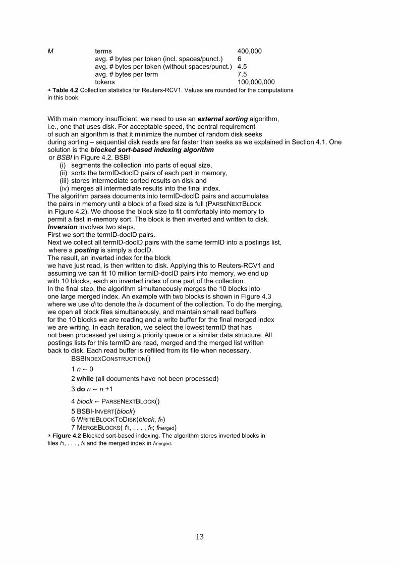
M terms 400,000 avg. # bytes per token (incl. spaces/punct.) 6 avg. # bytes per token (without spaces/punct.) 4.5 avg. # bytes per term 7.5 tokens 100,000,000

◮ Table 4.2 Collection statistics for Reuters-RCV1. Values are rounded for the computations in this book. With main memory insufficient, we need to use an external sorting algorithm, i.e., one that uses disk. For acceptable speed, the central requirement of such an algorithm is that it minimize the number of random disk seeks during sorting – sequential disk reads are far faster than seeks as we explained in Section 4.1. One solution is the blocked sort-based indexing algorithm or BSBI in Figure 4.2. BSBI

(i) segments the collection into parts of equal size, (ii) sorts the termID-docID pairs of each part in memory, (iii) stores intermediate sorted results on disk and (iv) merges all intermediate results into the final index.

The algorithm parses documents into termID-docID pairs and accumulates the pairs in memory until a block of a fixed size is full (PARSENEXTBLOCK in Figure 4.2). We choose the block size to fit comfortably into memory to permit a fast in-memory sort. The block is then inverted and written to disk. Inversion involves two steps. First we sort the termID-docID pairs. Next we collect all termID-docID pairs with the same termID into a postings list, where a posting is simply a docID. The result, an inverted index for the block we have just read, is then written to disk. Applying this to Reuters-RCV1 and assuming we can fit 10 million termID-docID pairs into memory, we end up with 10 blocks, each an inverted index of one part of the collection. In the final step, the algorithm simultaneously merges the 10 blocks into one large merged index. An example with two blocks is shown in Figure 4.3 where we use di to denote the ith document of the collection. To do the merging, we open all block files simultaneously, and maintain small read buffers for the 10 blocks we are reading and a write buffer for the final merged index we are writing. In each iteration, we select the lowest termID that has not been processed yet using a priority queue or a similar data structure. All postings lists for this termID are read, merged and the merged list written back to disk. Each read buffer is refilled from its file when necessary.

BSBINDEXCONSTRUCTION() 1 n ← 0 2 while (all documents have not been processed) 3 do n ← n +1

4 block ← PARSENEXTBLOCK() 5 BSBI-INVERT(block) 6 WRITEBLOCKTODISK(block, fn) 7 MERGEBLOCKS( f1, . . . , fn; fmerged)

◮ Figure 4.2 Blocked sort-based indexing. The algorithm stores inverted blocks in files f1, . . . , fn and the merged index in fmerged.

13

postings lists merged to be merged posting lists

brutus d1,d3 brutus d6,d7 brutus d1,d3,d6,d7 caesar d1,d2,d4 caesar d8,d9 caesar d1,d2,d4,d8,d9 noble d5 julius d10 julius d10 with d1,d2,d3,d5 killed d8 killed d8 noble d5 with d1,d2,d3,d5

DISK

◮Figure 4.3 Merging in blocked sort-based indexing. Two blocks (“postings lists to be merged”) are loaded from disk into memory, merged in memory (“merged postings lists”) and written back to disk. We show terms instead of termIDs for better readability.

5 Index compression

Chapter 1 introduced the dictionary and the inverted index as the central data structures in information retrieval. In this chapter, we employ a number of compression techniques for dictionary and inverted index that are essential for efficient IR systems. One benefit of compression is immediately clear. We will need less disk space. As we will see, compression ratios of 1:4 are easy to achieve, potentially cutting the cost of storing the index by 75%. There are two more subtle benefits of compression. The first is increased use of caching. Search systems use some parts of the dictionary and the index much more than others. For example, if we cache the postings list of a frequently used query term t, then the computations necessary for responding to the one-term query t can be entirely done in memory. With compression, we can fit a lot more information into main memory. Instead of having to expend a disk seek when processing a query with t, we instead access its postings list in memory and decompress it. As we will see below, there are simple and efficient decompression methods, so that the penalty (Nachteil) of having to decompress the postings list is small. As a result, we are able to decrease the response time of the IR system substantially. Since memory is a more expensive resource than disk space, increased speed due to caching – rather than decreased space requirements – is often the prime motivator for compression. The second more subtle advantage of compression is faster transfer of data from disk to memory. Efficient decompression algorithms run so fast on modern hardware that the total time of transferring a compressed chunk of data from disk and then decompressing it is usually less than transferring the same chunk of data in uncompressed form. For instance, we can reduce I/O time by loading a much smaller compressed postings list, even when you add on the cost of decompression. So in most cases, the retrieval system will run faster on compressed postings lists than on uncompressed postings lists. The compression algorithms we discuss in this chapter are highly efficient and can therefore serve all three purposes of index compression. In this chapter, we define a posting as a docID in a postings list. For example, the postings list (6; 20, 45, 100), where 6 is the termID of the list’s term, contains 3 postings. As discussed in Section 2.4.2 (page 41), postings in most search systems also contain frequency and position information; but we will only consider simple docID postings here.

14

5.1 Statistical properties of terms in information retrieval

(distinct) terms non-positional tokens ( = number of position Postings entries in postings)

number D% T% number D% T% number D% T% unfiltered 484,494 109,971,179 197,879,290 no numbers 473,723 −2 −2 100,680,242 −8 −8 179,158,204 −9 −9

case folding 391,523 −17 −19 96,969,056 −3 −12 179,158,204 −0 −9

30 stop words 391,493 −0 −19 83,390,443 −14 −24 121,857,825 −31 −38

150 stop words 391,373 −0 −19 67,001,847 −30 −39 94,516,599 −47 −52

stemming 322,383 −17 −33 63,812,300 −4 −42 94,516,599 −0 −52 ◮ Table 5.1 The effect of preprocessing on the number of terms, non-positional postings, and tokens for RCV1. “D%” indicates the reduction in size from the previous line, except that “30 stop words” and “150 stop words” both use “case folding” as their reference line. “T%” is the cumulative (“total”) reduction from unfiltered. We performed stemming with the Porter stemmer. The compression techniques we describe in the remainder of this chapter are lossless, that is, all information is preserved. 5.2 Dictionary compression The main goal of compressing the dictionary is to fit it in main memory, or at least a large portion of it, in order to support high query throughput (less disk accesses).

term document pointer to frequency postings list

a 656,265 → aachen 65 → . . . . . . . . . zulu 221 →

space needed: 20 bytes 4 bytes 4 bytes ◮ Figure 5.3 Storing the dictionary as an array of fixed-width entries.

For Reuters-RCV1, we need M× (20+ 4 + 4) = 400,000× 28 = 11.2MB for storing the dictionary in this scheme. Using fixed-width entries for terms is clearly wasteful. The average length of a term in English is about 8 characters , so on average we are wasting 12 characters in the fixed-width scheme. Also, we have no way of storing terms with more than 20 characters like hydrochlorofluorocarbons and supercalifragilisticexpialidocious. We can overcome these shortcomings by storing the dictionary terms as one long string of characters, as shown in Figure 5.4.

15

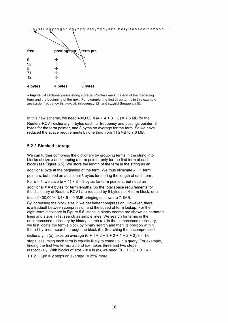
. . . s y s t i l e s y z y g e t i c s y z y g i a l s y z y g y s z a i b e l y i t e s z e c i n s z o n o . . . freq. postings ptr. term ptr. 9 92 5 71 12 . . . … … 4 bytes 4 bytes 3 bytes ◮ Figure 5.4 Dictionary-as-a-string storage. Pointers mark the end of the preceding term and the beginning of the next. For example, the first three terms in this example are systile (frequency 9), syzygetic (frequency 92) and syzygial (frequency 5). In this new scheme, we need 400,000 × (4 + 4 + 3 + 8) = 7.6 MB for the Reuters-RCV1 dictionary: 4 bytes each for frequency and postings pointer, 3 bytes for the term pointer, and 8 bytes on average for the term. So we have reduced the space requirements by one third from 11.2MB to 7.6 MB. 5.2.2 Blocked storage We can further compress the dictionary by grouping terms in the string into blocks of size k and keeping a term pointer only for the first term of each block (see Figure 5.5). We store the length of the term in the string as an additional byte at the beginning of the term. We thus eliminate k − 1 term pointers, but need an additional k bytes for storing the length of each term. For k = 4, we save (k − 1) × 3 = 9 bytes for term pointers, but need an additional k = 4 bytes for term lengths. So the total space requirements for the dictionary of Reuters-RCV1 are reduced by 5 bytes per 4-term block, or a total of 400,000× 1/4× 5 = 0.5MB bringing us down to 7.1MB. By increasing the block size k, we get better compression. However, there is a tradeoff between compression and the speed of term lookup. For the eight-term dictionary in Figure 5.6, steps in binary search are shown as cornered lines and steps in list search as simple lines. We search for terms in the uncompressed dictionary by binary search (a). In the compressed dictionary, we first locate the term’s block by binary search and then its position within the list by linear search through the block (b). Searching the uncompressed dictionary in (a) takes on average (0 + 1 + 2 + 3 + 2 + 1 + 2 + 2)/8 ≈ 1.6 steps, assuming each term is equally likely to come up in a query. For example, finding the first two terms, aid and box, takes three and two steps, respectively. With blocks of size k = 4 in (b), we need (0 + 1 + 2 + 3 + 4 + 1 + 2 + 3)/8 = 2 steps on average, ≈ 25% more.

16

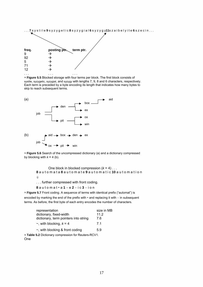
. . . 7 s y s t i l e 9 s y z y g e t i c 8 s y z y g i a l 6 s y z y g y11s z a i b e l y i t e 6 s z e c i n . . . freq. posting ptr. term ptr. 9 92 5 71 12 . . . . . . . . . ◮ Figure 5.5 Blocked storage with four terms per block. The first block consists of systile, syzygetic, syzygial, and syzygy with lengths 7, 9, 8 and 6 characters, respectively. Each term is preceded by a byte encoding its length that indicates how many bytes to skip to reach subsequent terms. (a) aid

box den

ex job

ox pit

win

(b) aid box den ex

job ox pit win

◮ Figure 5.6 Search of the uncompressed dictionary (a) and a dictionary compressed by blocking with k = 4 (b).

One block in blocked compression (k = 4) . . . 8 a u t o m a t a 8 a u t o m a t e 9 a u t o m a t i c 10 a u t o m a t i o n ⇓ . . . further compressed with front coding. 8 a u t o m a t ∗ a 1 ⋄ e 2 ⋄ i c 3 ⋄ i o n

◮ Figure 5.7 Front coding. A sequence of terms with identical prefix (“automat”) is encoded by marking the end of the prefix with ∗ and replacing it with ⋄ in subsequent terms. As before, the first byte of each entry encodes the number of characters.

representation size in MB dictionary, fixed-width 11.2 dictionary, term pointers into string 7.6 ∼, with blocking, k = 4 7.1

∼, with blocking & front coding 5.9 ◮ Table 5.2 Dictionary compression for Reuters-RCV1. One

17

5.3 Postings file compression 5.3.1 Variable byte codes

VBENCODENUMBER(n) 1 bytes ← [] 2 while true 3 do PREPEND(bytes, n mod 128) 4 if n < 128 5 then BREAK

6 n ← n div 128 7 bytes[LENGTH(bytes)] += 128 8 return bytes VBENCODE(numbers) 1 bytestream ← [] 2 for each n ∈ numbers

3 do bytes ← VBENCODENUMBER(n)

4 bytestream ← EXTEND(bytestream, bytes) 5 return bytestream

VBDECODE(bytestream) 1 numbers ← [] 2 n ← 0

3 for i ← 1 to LENGTH(bytestream) 4 do if bytestream[i] < 128 5 then n ← 128× n + bytestream[i]

6 else n ← 128× n + (bytestream[i] − 128) 7 APPEND(numbers, n) 8 n ← 0 9 return numbers

◮ Figure 5.8 Variable byte encoding and decoding. The functions div and mod compute integer division and remainder after integer division, respectively. Prepend adds an element to the beginning of a list, e.g., PREPREND(h1,2i, 3) = h3, 1, 2i. Extend

extends a list, e.g., EXTEND(<1,2>, <3, 4>) = <1, 2, 3, 4>.

docIDs 824 829 215406 gaps 5 214577 VB code 00000110 10111000 10000101 00001101 00001100 10110001

◮ Table 5.4 Variable byte (VB) encoding. Gaps are encoded using an integral number of bytes. The first bit, the continuation bit, of each byte indicates whether the code ends with this byte (1) or not (0). 5.3.2 ɣ codes Variable byte codes use an adaptive number of bytes depending on the size of the gap. Bit-level codes adapt the length of the code on the finer grained bit level. The simplest bit-level code is unary code. The unary code of n is a string

18

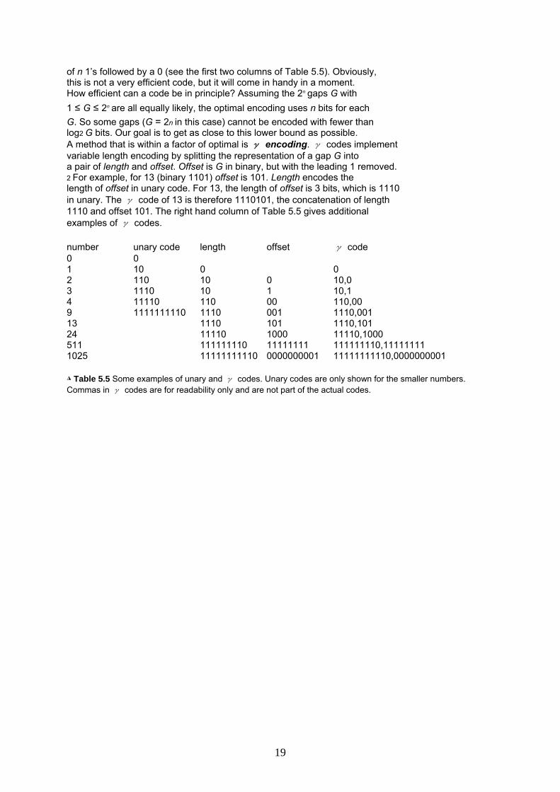
of n 1’s followed by a 0 (see the first two columns of Table 5.5). Obviously, this is not a very efficient code, but it will come in handy in a moment. How efficient can a code be in principle? Assuming the 2n gaps G with 1 ≤ G ≤ 2n are all equally likely, the optimal encoding uses n bits for each G. So some gaps (G = 2n in this case) cannot be encoded with fewer than log2 G bits. Our goal is to get as close to this lower bound as possible. A method that is within a factor of optimal is γ encoding. γ codes implement variable length encoding by splitting the representation of a gap G into a pair of length and offset. Offset is G in binary, but with the leading 1 removed. 2 For example, for 13 (binary 1101) offset is 101. Length encodes the length of offset in unary code. For 13, the length of offset is 3 bits, which is 1110 in unary. The γ code of 13 is therefore 1110101, the concatenation of length 1110 and offset 101. The right hand column of Table 5.5 gives additional examples of γ codes. number unary code length offset γ code 0 0 1 10 0 0 2 110 10 0 10,0 3 1110 10 1 10,1 4 11110 110 00 110,00 9 1111111110 1110 001 1110,001 13 1110 101 1110,101 24 11110 1000 11110,1000 511 111111110 11111111 111111110,11111111 1025 11111111110 0000000001 11111111110,0000000001

◮ Table 5.5 Some examples of unary and γ codes. Unary codes are only shown for the smaller numbers. Commas in γ codes are for readability only and are not part of the actual codes.

19

6 Scoring, term weighting and the vector space model So far we have dealt with indexes that support Boolean queries: a document either matches or does not match a query. In the case of large document collections, the resulting number of matching documents can far exceed the number a human user could possibly sift through. Accordingly, it is essential for a search engine to rank-order the documents matching a query. To do this, the search engine computes, for each matching document, a score with respect to the query at hand. In this chapter we initiate the study of assigning a score to a (query, document) pair. 6.1 Parametric and zone indexes So far we viewed a document as a sequence of terms. Most documents have additional structure. Digital documents generally encode, in machine-recognizable form, certain metadata associated with each document. By metadata, we mean specific forms of data about a document, such as its author(s), title and date of publication. This metadata would generally include fields such as the date of creation and the format of the document, as well the author and possibly the title of the document. Consider queries of the form “find documents authored by William Shakespeare in 1601, containing the phrase alas poor Yorick”. Query processing then consists as usual of postings intersections, except that we may merge postings from standard inverted as well as parametric indexes (e.g. B-trees). Zones are similar to fields, except the contents of a zone can be arbitrary free text. Whereas a field may take on a relatively small set of values, a zone can be thought of as an arbitrary, unbounded amount of text. Examples:document titles and abstracts

Figure 6.1 Parametric search. In this example we have a collection with fields allowing us to select publications by zones such as Author and fields such as Language.

20

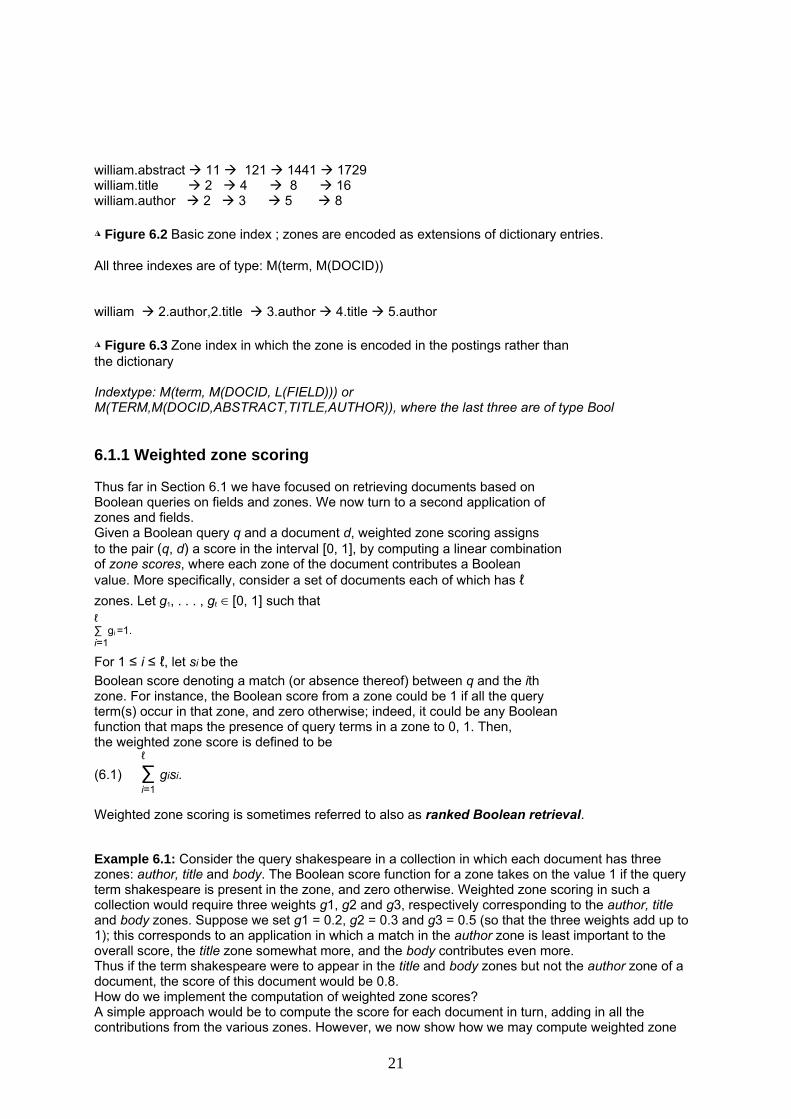
william.abstract 11 121 1441 1729 william.title 2 4 8 16 william.author 2 3 5 8

◮ Figure 6.2 Basic zone index ; zones are encoded as extensions of dictionary entries. All three indexes are of type: M(term, M(DOCID)) william 2.author,2.title 3.author 4.title 5.author

◮ Figure 6.3 Zone index in which the zone is encoded in the postings rather than the dictionary Indextype: M(term, M(DOCID, L(FIELD))) or M(TERM,M(DOCID,ABSTRACT,TITLE,AUTHOR)), where the last three are of type Bool 6.1.1 Weighted zone scoring Thus far in Section 6.1 we have focused on retrieving documents based on Boolean queries on fields and zones. We now turn to a second application of zones and fields. Given a Boolean query q and a document d, weighted zone scoring assigns to the pair (q, d) a score in the interval [0, 1], by computing a linear combination of zone scores, where each zone of the document contributes a Boolean value. More specifically, consider a set of documents each of which has ℓ zones. Let g1, . . . , gℓ ∈ [0, 1] such that ℓ ∑ g =1. i i=1 For 1 ≤ i ≤ ℓ, let si be the Boolean score denoting a match (or absence thereof) between q and the ith zone. For instance, the Boolean score from a zone could be 1 if all the query term(s) occur in that zone, and zero otherwise; indeed, it could be any Boolean function that maps the presence of query terms in a zone to 0, 1. Then, the weighted zone score is defined to be

ℓ

(6.1) ∑ gisi. i=1

Weighted zone scoring is sometimes referred to also as ranked Boolean retrieval. Example 6.1: Consider the query shakespeare in a collection in which each document has three zones: author, title and body. The Boolean score function for a zone takes on the value 1 if the query term shakespeare is present in the zone, and zero otherwise. Weighted zone scoring in such a collection would require three weights g1, g2 and g3, respectively corresponding to the author, title and body zones. Suppose we set g1 = 0.2, g2 = 0.3 and g3 = 0.5 (so that the three weights add up to 1); this corresponds to an application in which a match in the author zone is least important to the overall score, the title zone somewhat more, and the body contributes even more. Thus if the term shakespeare were to appear in the title and body zones but not the author zone of a document, the score of this document would be 0.8. How do we implement the computation of weighted zone scores? A simple approach would be to compute the score for each document in turn, adding in all the contributions from the various zones. However, we now show how we may compute weighted zone

21

scores directly from inverted indexes. The algorithm of Figure 6.4 treats the case when the query q is a two term query consisting of query terms q1 and q2, and the Boolean function is AND: 1 if both query terms are present in a zone and 0 otherwise.

ZONESCORE(q1, q2) 1 float scores[N] = [0] 2 constant g[ℓ] 3 p1 ← postings(q1)

4 p2 ← postings(q2) 5 // scores[] is an array with a score entry for each document, initialized to zero. 6 // p1 and p2 are initialized to point to the beginning of their respective postings. 7 // Assume g[] is initialized to the respective zone weights. 8 while p1 != NIL and p2 != NIL

9 do if docID(p1) = docID(p2) 10 then scores[docID(p1)] ← WEIGHTEDZONE(p1, p2, g)

11 p1 ← next(p1)

12 p2 ← next(p2) 13 else if docID(p1) < docID(p2) 14 then p1 ← next(p1)

15 else p2 ← next(p2) 16 return scores

◮ Figure 6.4 Algorithm for computing the weighted zone score from two postings lists. Function WEIGHTEDZONE (not shown here) is assumed to compute the inner loop of Equation 6.1. 6.2 Term frequency and weighting We assign to each term in a document a weight for that term that depends on the number of occurrences of the term in the document. We would like to compute a score between a query term t and a document d, based on the weight of t in d. The simplest approach is to assign the weight to be equal to the number of occurrences of term t in document d. This weighting scheme is referred to as term frequency and is denoted tft,d with the subscripts denoting the term and the document in order. For a document d, the set of weights determined by the tf weights above (or indeed any weighting function that maps the number of occurrences of t in d to a positive real value) may be viewed as a quantitative digest (Kurzfassung) of that BAG OF WORDS document. In this view of a document, known in the literature as the bag of words model, the exact ordering of the terms in a document is ignored but the number of occurrences of each term is material (in contrast to Boolean retrieval). We only retain (aufbewahren) information on the number of occurrences of each term. Thus, the document “Mary is quicker than John” is, in this view, identical to the document “John is quicker than Mary”. Nevertheless, it seems intuitive that two documents with similar bag of words representations are similar in content. 6.2.1 Inverse document frequency Raw term frequency as above suffers from a critical problem: all terms are considered equally important when it comes to assessing relevancy on a query. In fact certain terms have little or no discriminating power in determining relevance. For instance, a collection of documents on the auto industry is likely to have the term auto in almost every document. To this end, we introduce a mechanism for attenuating (abmildern) the effect of terms that occur too often in the collection to be meaningful for relevance determination. An immediate idea is to scale down the term weights of terms with high collection frequency, defined to be the total number of occurrences of a term in the collection. The idea would be to reduce the tf weight of a term by a factor that grows with its collection frequency.

22

Instead, it is more commonplace to use for this purpose the document frequency dft, defined to be the number of documents in the collection that contain a term t. This is because in trying to discriminate between documents for the purpose of scoring it is better to use a document-level statistic (such as the number of documents containing a term) than to use a collection-wide statistic for the term. The reason to prefer df to cf is illustrated in Figure 6.7,

Word cf df try 10422 8760 insurance 10440 3997

◮ Figure 6.7 Collection frequency (cf) and document frequency (df) behave differently, as in this example from the Reuters collection. where a simple example shows that collection frequency (cf) and document frequency (df) can behave rather differently. In particular, the cf values for both try and insurance are roughly equal, but their df values differ significantly. Intuitively, we want the few documents that contain insurance to get a higher boost for a query on insurance than the many documents containing try get from a query on try. How is the document frequency df of a term used to scale its weight? Denoting as usual the total number of documents in a collection by N,we define the inverse document frequency (idf) of a term t as follows: (6.7) idft = log N

dft Thus the idf of a rare term is high, whereas the idf of a frequent term is likely to be low. Figure 6.8 gives an example of idf’s in the Reuters collection of 806,791 documents; in this example logarithms are to the base 10. In fact, as we will see in Exercise 6.12, the precise base of the logarithm is not material to ranking. We will give on page 227 a justification of the particular form in Equation (6.7).

term dft Idft car 18,165 1.65 auto 6723 2.08 insurance 19,241 1.62 best 25,235 1.5

◮ Figure 6.8 Example of idf values. Here we give the idf’s of terms with various frequencies in the Reuters collection of 806,791 documents. 6.3 The vector space model for scoring We denote by ~V (d) the vector derived from document d, with one component in the vector for each dictionary term. Unless otherwise specified, the reader may assume that the components are computed using the tf-idf weighting scheme, although the particular weighting scheme is immaterial to the discussion that follows. The set of documents in a collection then may be viewed as a set of vectors in a vector space, in which there is one axis for each term. This representation loses the relative ordering of the terms in each document; recall our example from Section 6.2 (page 117), where we pointed out that the documents Mary is quicker than John and John is quicker than Mary are identical in such a bag of words representation. How do we quantify the similarity between two documents in this vector space? A first attempt might consider the magnitude of the vector difference between two document vectors. This measure suffers from a drawback: two documents with very similar content can have a significant vector difference simply because one is much longer than the other. Thus the relative distributions of terms may be identical in the two documents, but the absolute term frequencies of one may be far larger. To compensate for the effect of document length, the standard way of quantifying the similarity between two documents d1 and d2 is to compute the cosine similarity of their vector representations ~V (d1) and ~V (d2)

23

24

(6.10) sim(d1, d2) = ~V(d1) · ~V (d2)

|~V (d1)||~V (d2)|

where the numerator represents the dot product (also known as the inner product) of the vectors ~V(d1) and ~V (d2), while the denominator is the product of their Euclidean lengths. The dot product ~x · ~y of two vectors is defined as

M ∑ xi y i

i=1 The effect of the denominator of Equation (6.10) is thus to length-normalize the vectors ~V(d1) and ~V(d2) to unit vectors ~v(d1) = ~V (d1)/|~V(d1)| and

Doc1 Doc2 Doc3 car 0.88 0.09 0.58 auto 0.10 0.71 0 insurance 0 0.71 0.70 best 0.46 0 0.41

◮ Figure 6.11 Euclidean normalized tf values for documents in Figure 6.9.

term SaS PaP WH affection 115 58 20 jealous 10 7 11 gossip 2 0 6

◮ Figure 6.12 Term frequencies in three novels. The novels are Austen’s Sense and Sensibility, Pride and Prejudice and Bronte’sWuthering Heights.

~v(d2) = ~V (d2)/|~V (d2)|. We can then rewrite (6.10) as

sim(d1, (6.11) d2) = ~v(d1) ·~v(d2). To summarize, by viewing a query as a “bag of words”, we are able to treat it as a very short document. As a consequence, we can use the cosine similarity between the query vector and a document vector as a measure of the score of the document for that query. The resulting scores can then be used to select the top-scoring documents for a query. Thus we have ~V(q) · ~V (d)

(6.12) score(q, d) = |~V (q)||~V(d)|