1

Automatic Speech Recognition: An Overview

Julia Hirschberg

CS 4706

(special thanks to Roberto Pieraccini)

2

Recreating the Speech Chain DIALOG

SEMANTICS

SYNTAX

LEXICON

MORPHOLOGY

PHONETICS

VOCAL-TRACTARTICULATORS

INNER EARACOUSTIC

NERVE

SPEECHRECOGNITION

DIALOGMANAGEMENT

SPOKENLANGUAGE

UNDERSTANDING

SPEECHSYNTHESIS

3

Speech Recognition: the Early Years

• 1952 – Automatic Digit Recognition (AUDREY)– Davis, Biddulph,

Balashek (Bell Laboratories)

4

1960’s – Speech Processing and Digital Computers

AD/DA converters and digital computers start appearing in the labs

James FlanaganBell Laboratories

5

The Illusion of Segmentation... or...

Why Speech Recognition is so Difficult

m I n & m b

& r i s e v & n th

r E n I n z E r

o t ü s e v & n f O r

MY

NUMBER

IS

SEVEN

THREE

NINE

ZERO

TWO

SEVEN

FOUR

NPNP

VP

(user:Roberto (attribute:telephone-num value:7360474))(user:Roberto (attribute:telephone-num value:7360474))

6

The Illusion of Segmentation... or...

Why Speech Recognition is so Difficult

m I n & m b

& r i s e v & n th

r E n I n z E r

o t ü s e v & n f O r

MY

NUMBER

IS

SEVEN

THREE

NINE

ZERO

TWO

SEVEN

FOUR

NPNP

VP

(user:Roberto (attribute:telephone-num value:7360474))(user:Roberto (attribute:telephone-num value:7360474))

Intra-speaker variability

Noise/reverberation

Coarticulation

Context-dependency

Word confusability

Word variations

Speaker Dependency

Multiple Interpretations

Limited vocabulary

Ellipses and Anaphors

7

1969 – Whither Speech Recognition? General purpose speech recognition seems far away. Social-

purpose speech recognition is severely limited. It would seem appropriate for people to ask themselves why they are working in the field and what they can expect to accomplish…

It would be too simple to say that work in speech recognition is carried out simply because one can get money for it. That is a necessary but not sufficient condition. We are safe in asserting that speech recognition is attractive to money. The attraction is perhaps similar to the attraction of schemes for turning water into gasoline, extracting gold from the sea, curing cancer, or going to the moon. One doesn’t attract thoughtlessly given dollars by means of schemes for cutting the cost of soap by 10%. To sell suckers, one uses deceit and offers glamour…

Most recognizers behave, not like scientists, but like mad inventors or untrustworthy engineers. The typical recognizer gets it into his head that he can solve “the problem.” The basis for this is either individual inspiration (the “mad inventor” source of knowledge) or acceptance of untested rules, schemes, or information (the untrustworthy engineer approach).

The Journal of the Acoustical Society of America, June 1969

J. R. PierceExecutive Director,Bell Laboratories

8

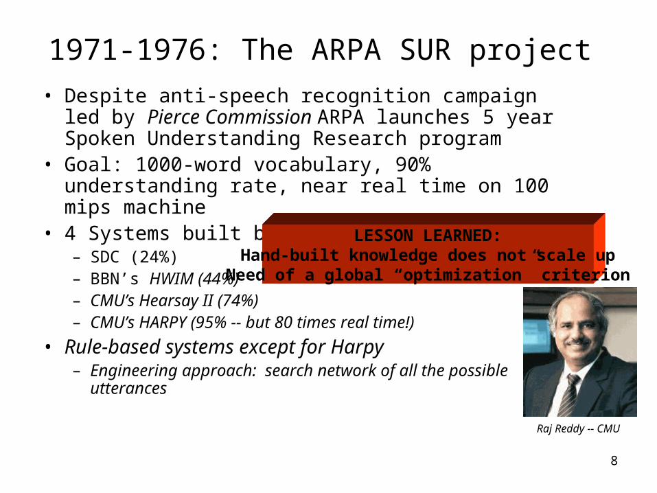
1971-1976: The ARPA SUR project

• Despite anti-speech recognition campaign led by Pierce Commission ARPA launches 5 year Spoken Understanding Research program

• Goal: 1000-word vocabulary, 90% understanding rate, near real time on 100 mips machine

• 4 Systems built by the end of the program– SDC (24%)– BBN’s HWIM (44%)– CMU’s Hearsay II (74%)– CMU’s HARPY (95% -- but 80 times real time!)

• Rule-based systems except for Harpy– Engineering approach: search network of all the

possible utterances

Raj Reddy -- CMU

LESSON LEARNED:Hand-built knowledge does not scale upNeed of a global “optimization” criterion

9

• Lack of clear evaluation criteria– ARPA felt systems had failed– Project not extended

• Speech Understanding: too early for its time• Need a standard evaluation method

10

1970’s – Dynamic Time WarpingThe Brute Force of the Engineering Approach

TE

MP

LAT

E (

WO

RD

7)

UNKNOWN WORD

T.K. Vyntsyuk (1968)H. Sakoe, S. Chiba (1970)

Isolated WordsSpeaker Dependent

Connected WordsSpeaker Independent

Sub-Word Units

11

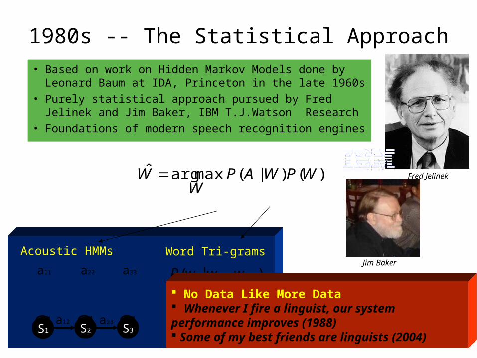
1980s -- The Statistical Approach

• Based on work on Hidden Markov Models done by Leonard Baum at IDA, Princeton in the late 1960s

• Purely statistical approach pursued by Fred Jelinek and Jim Baker, IBM T.J.Watson Research

• Foundations of modern speech recognition engines

)()|(maxargˆ WPWAPW

W Fred Jelinek

S1 S2 S3

a11

a12

a22

a23

a33 ),|( 21 ttt wwwP

Acoustic HMMs Word Tri-grams

No Data Like More Data Whenever I fire a linguist, our system performance improves (1988) Some of my best friends are linguists (2004)

Jim Baker

12

1980-1990 – Statistical approach becomes ubiquitous

• Lawrence Rabiner, A Tutorial on Hidden Markov Models and Selected Applications in Speech Recognition, Proceeding of the IEEE, Vol. 77, No. 2, February 1989.

13

1980s-1990s – The Power of Evaluation

Pros and Cons of DARPA programs

+ Continuous incremental improvement- Loss of “bio-diversity”

SPOKENDIALOGINDUSTRY

SPEECHWORKS

NUANCE

MIT

SRI

TECHNOLOGYVENDORS

PLATFORMINTEGRATORS

APPLICATIONDEVELOPERS

HOSTING

TOOLS

STANDARDS

STANDARDS

STANDARDS

1997

19951996

19981999

20002001

20022003

2004…

14

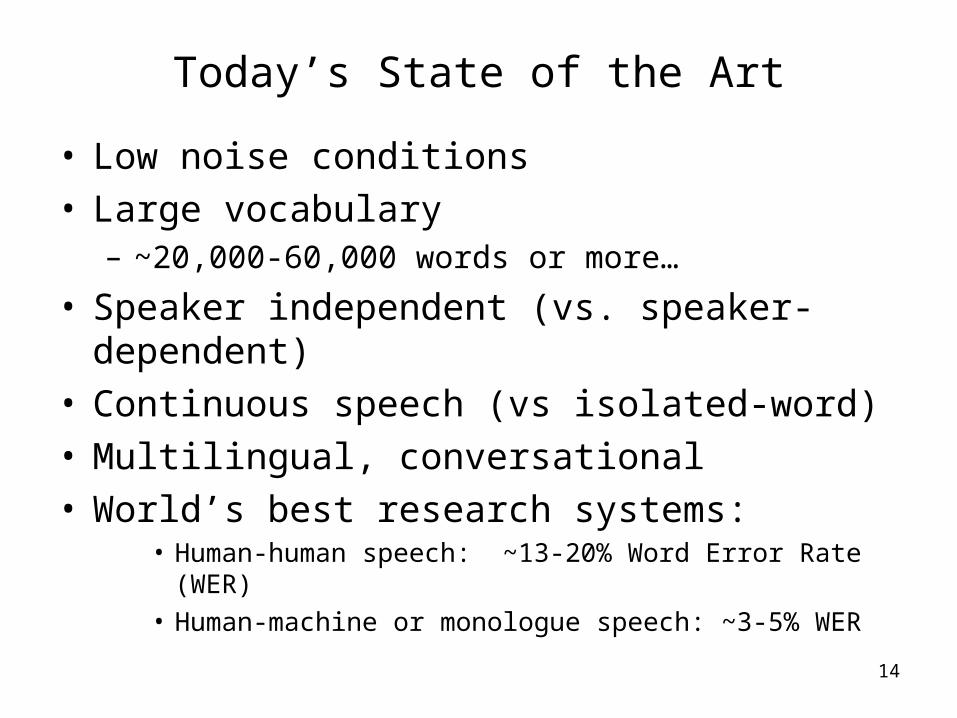
Today’s State of the Art

• Low noise conditions• Large vocabulary

– ~20,000-60,000 words or more…

• Speaker independent (vs. speaker-dependent)• Continuous speech (vs isolated-word)• Multilingual, conversational• World’s best research systems:

• Human-human speech: ~13-20% Word Error Rate (WER)• Human-machine or monologue speech: ~3-5% WER

15

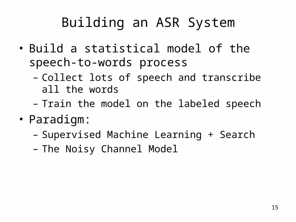
Building an ASR System

• Build a statistical model of the speech-to-words process– Collect lots of speech and transcribe all the words– Train the model on the labeled speech

• Paradigm: – Supervised Machine Learning + Search– The Noisy Channel Model

16

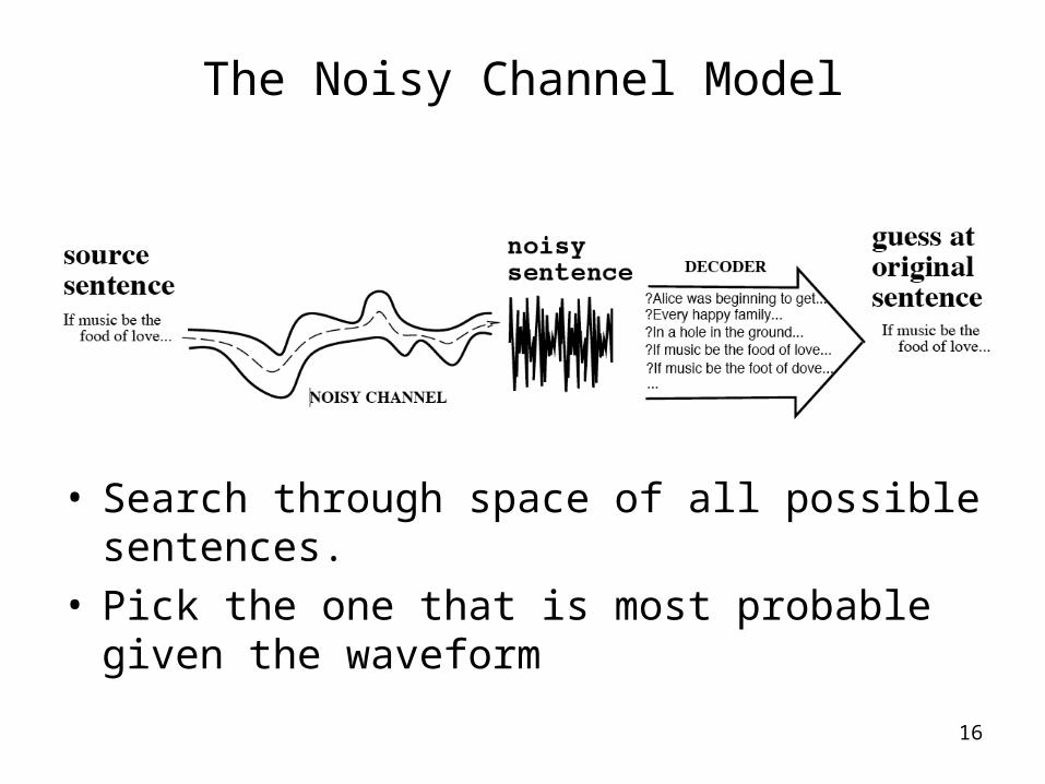
The Noisy Channel Model

• Search through space of all possible sentences.• Pick the one that is most probable given the

waveform

17

The Noisy Channel Model (II)

• What is the most likely sentence out of all sentences in the language L, given some acoustic input O?

• Treat acoustic input O as sequence of individual acoustic observations – O = o1,o2,o3,…,ot

• Define a sentence as a sequence of words:– W = w1,w2,w3,…,wn

18

Noisy Channel Model (III)

• Probabilistic implication: Pick the highest probable sequence:

• We can use Bayes rule to rewrite this:

• Since denominator is the same for each candidate sentence W, we can ignore it for the argmax:

ˆ W argmaxW L

P(W | O)

ˆ W argmaxW L

P(O |W )P(W )

ˆ W argmaxW L

P(O |W )P(W )

P(O)

19

Speech Recognition Meets Noisy Channel: Acoustic Likelihoods and LM Priors

20

Components of an ASR System

• Corpora for training and testing of components• Representation for input and method of

extracting• Pronunciation Model• Acoustic Model• Language Model• Feature extraction component• Algorithms to search hypothesis space efficiently

21

Training and Test Corpora

• Collect corpora appropriate for recognition task at hand– Small speech + phonetic transcription to associate

sounds with symbols (Acoustic Model)– Large (>= 60 hrs) speech + orthographic transcription

to associate words with sounds (Acoustic Model)– Very large text corpus to identify ngram probabilities

or build a grammar (Language Model)

22

Building the Acoustic Model

• Goal: Model likelihood of sounds given spectral features, pronunciation models, and prior context

• Usually represented as Hidden Markov Model– States represent phones or other subword units– Transition probabilities on states: how likely is it to

see one sound after seeing another?– Observation/output likelihoods: how likely is spectral

feature vector to be observed from phone state i, given phone state i-1?

23

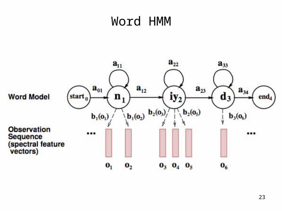
Word HMM

24

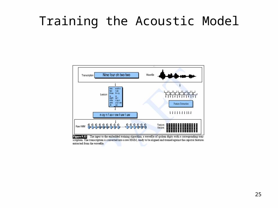
• Initial estimates from phonetically transcribed corpus or flat start– Transition probabilities between phone states– Observation probabilities associating phone states

with acoustic features of windows of waveform

• Embedded training: – Re-estimate probabilities using initial phone HMMs

+ orthographically transcribed corpus + pronunciation lexicon to create whole sentence HMMs for each sentence in training corpus

– Iteratively retrain transition and observation probabilities by running the training data through the model until convergence

25

Training the Acoustic Model

26

Building the Pronunciation Model

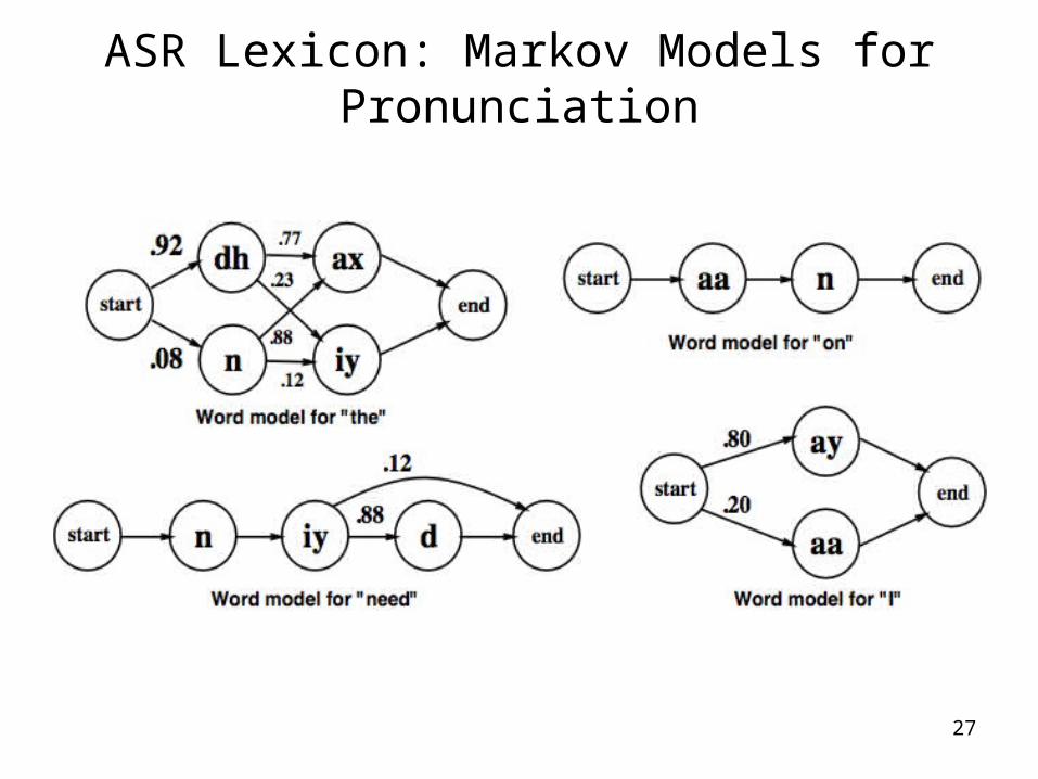
• Models likelihood of word given network of candidate phone hypotheses – Multiple pronunciations for each word– May be weighted automaton or simple dictionary

• Words come from all corpora (including text)• Pronunciations come from pronouncing

dictionary or TTS system

27

ASR Lexicon: Markov Models for Pronunciation

28

Building the Language Model

• Models likelihood of word given previous word(s)• Ngram models:

– Build the LM by calculating bigram or trigram probabilities from text training corpus: how likely is one word to follow another? To follow the two previous words?

– Smoothing issues

• Grammars– Finite state grammar or Context Free Grammar

(CFG) or semantic grammar

• Out of Vocabulary (OOV) problem

29

Search/Decoding

• Find the best hypothesis P(O|W) P(W) given– A sequence of acoustic feature vectors (O)– A trained HMM (AM)– Lexicon (PM)– Probabilities of word sequences (LM)

• For O– Calculate most likely state sequence in HMM given transition

and observation probs – Trace back thru state sequence to assign words to states– N best vs. 1 best vs. lattice output

• Limiting search– Lattice minimization and determinization– Pruning: beam search

30

Evaluating Success

• Transcription – Low WER (Subst+Ins+Del)/N * 100

Thesis test vs. This is a test. 75% WER

Or That was the dentist calling. 125% WER

• Understanding– High concept accuracy

• How many domain concepts were correctly recognized?

I want to go from Boston to Baltimore on September 29

31

Domain concepts Values– source city Boston– target city Baltimore– travel date September 29– Score recognized string “Go from Boston to

Washington on December 29” vs. “Go to Boston from Baltimore on September 29”

– (1/3 = 33% CA)

32

Summary

• ASR today– Combines many probabilistic phenomena: varying

acoustic features of phones, likely pronunciations of words, likely sequences of words

– Relies upon many approximate techniques to ‘translate’ a signal

– Finite State Transducers

• ASR future– Can we include more language phenomena in the

model?

33

Next Class

• Speech disfluencies: a challenge for ASR