1

Artifacts and Textured Region Detection

Vishal Bangard

ECE 738 - Spring 2003

I. INTRODUCTION

A lot of transformations, when applied to images, lead to the development of various artifacts in them. In

particular, we will be addressing artifacts caused by compression algorithms. Few of the artifacts [1] caused

by popular compression algorithms are:

• Blocking artifacts: Some compression algorithms divide an image into blocks of a definite size. E.g.

JPEG works on 8x8 blocks at a time. This leads to the resulting compressed image having a very “blocky”

appearance.

• Color Distortion: Human eyes are not as sensitive to color as to brightness. As a result, much of the

detailed color (chrominance) information is disposed, while luminance information is retained. This

process is called ”chroma subsampling”. The result of this is that compressed pictures have a “washed

out” appearance, in which the colors do not look as bright as in the original image.

• Ringing Artifacts: Quite a few times, compression algorithms that work in the spectral domain take

advantage of the fact that low frequency information is visually more important than the high frequency

information. Some of them try to exploit this fact and do not retain all the high frequency information.

This leads to distortions in edges and other boundaries.

• Blurring Artifacts: With the presence of these artifacts, the image looks smoother than the original coun-

terpart. The general shape of objects is correctly retained, but the texture information is lost in some

areas.

A lot of work has been previously done to tackle blocking artifacts, color distortion and ringing artifacts.

To repair the effects of Blurring artifacts, there are existing methods for texture synthesis, or replication of

texture in an area based on information from adjacent regions. However, most of the existing algorithms

require the source and destination areas for texture synthesis to be marked out manually. The aim of this

project is to identify regions near textured areas as these have a higher probability of being subject to texture

loss. A completely automated detection system is very hard due to the highly subjective nature of this problem.

2

II. HIGH FREQUENCY ANALYSIS

Textured areas generally have a lot more high frequencies as compared to smooth areas. Hence, one of the

approaches adopted was to analyze the high frequency component of the image.

A standard wavelet decomposition was used and the sum of the squares of the high frequency coefficients

was found. This gave an indication as to the amount of energy that was being contributed by the high frequency

components. It was conjectured that a textured region would have a large amount of energy contributed due

to these high frequencies. This analysis was done on an 8x8 block basis as this eased computation and also

kept a direct link between the spectral and the spatial domains.

To see the potential of this method, the image was thresholded to show the best results.

The results seen using this method seemed encouraging. However, one of the primary drawbacks of this

method was low resolution. Each 8x8 block was classified as rich in high frequencies or not. Going to lower

block sizes (i.e. 4x4 and 2x2) leaves very few high frequency coefficients to get reliable results. Also, this

technique in itself did not give good edge detection, which also forms an essential part in obtaining nearby

regions.

Another problem was that some small areas were missed as being detected as textured or not. The most

likely reason for this may be the minimum resolution being 8x8 due to the choice of block size.

III. GABOR WAVELET ANALYSIS

Another approach for texture detection was to find the Gabor wavelet decomposition of the image. The

Gabor elementary functions are able to closely model the anisotropic two dimensional receptive fields of

neurons in the mammalian visual cortex. (The first experiment towards this was successfully conducted by J.

P. Jones and L. A. Palmer, on the visual cortex of a cat [2]. Later experiments have been performed on other

mammals including monkeys and reinforce these results.)

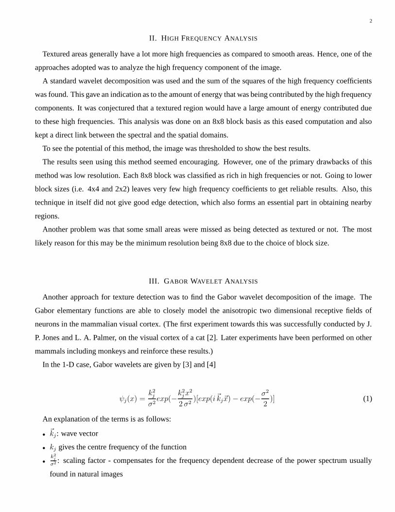
In the 1-D case, Gabor wavelets are given by [3] and [4]

ψj(x) =k2

j

σ2exp(−

k2

jx2

2 σ2)[exp(i~kj~x) − exp(−

σ2

2)] (1)

An explanation of the terms is as follows:

•~kj: wave vector

• kj gives the centre frequency of the function

•

k2

j

σ2 : scaling factor - compensates for the frequency dependent decrease of the power spectrum usually

found in natural images

3

(a) Image: Barbara (b) Image (a) compressed at 1:94. Observe the loss in

texture in the lady’s clothing and the tablecloth.

(c) Solid black areas give edges and regions of high tex-

ture

(d) An edge map of image (c) overlaid on the com-

pressed image

Fig. 1. The image Barbara subjected to high frequency analysis

4

−20 −10 0 10 20−20020

−0.01

−0.005

0

0.005

0.01

0.015

(a) Real component of the Gabor filter

−20 −10 0 10 20−20020

−0.015

−0.01

−0.005

0

0.005

0.01

0.015

(b) Imaginary component of the Gabor filter

Fig. 2. Gabor filters (These were generated using a filter width of 41 and variances 10 in the x and y directions)

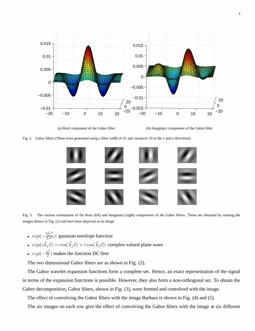
Fig. 3. The various orientations of the Real (left) and Imaginary (right) components of the Gabor filters. These are obtained by rotating the

images shown in Fig. (2) and have been depicted as an image

• exp(−k2

jx2

2 σ2 ): gaussian envelope function

• exp(i ~kj~x) = cos(~kj~x) + i cos(~kj~x): complex-valued plane wave

• exp(−σ2

2) makes the function DC-free

The two dimensional Gabor filters are as shown in Fig. (2).

The Gabor wavelet expansion functions form a complete set. Hence, an exact representation of the signal

in terms of the expansion functions is possible. However, they also form a non-orthogonal set. To obtain the

Gabor decomposition, Gabor filters, shown in Fig. (3), were formed and convolved with the image.

The effect of convolving the Gabor filters with the image Barbara is shown in Fig. (4) and (5).

The six images on each row give the effect of convolving the Gabor filters with the image at six different

5

Fig. 4. The magnitude of the result of convolving the image with the Gabor filters at six different orientations and four different scales

orientations. This is done for four different scales and shown here. It is seen in Fig. (4) that the lady’s clothing

is captured very well on the first two scales, but the tablecloth barely shows up on them. On scale three and

four, the tablecloth is detected well, but the clothing is barely detected. Hence, it is necessary to implement

the Gabor filters at more than one scale, and convolve them with the image. The frequency of the complex

sinusoid, and hence the number of scales used imposes a limit on the type of texture that can be detected by

these filters. This is seen when some of the textures are detected on one scale, but not the other.

Different parts of the texture show up on different orientations. To detect all the textured regions, it is

necessary to combine all of them. To do this, for each scale, we took the maximum of the values obtained in

each orientation, and rescaled the result.

Another thing that was found to be useful was the phase information generated using the Gabor filters. The

phase information is combined in a similar manner as the magnitude information was. At the lower two scales,

it was found that the phase information can be used to detect some edges and textured regions too.

In our implementation, the magnitude information from various scales was combined by taking the maxi-

mum across the various scales. The phase information from the first scale was the only one used. These were

6

Fig. 5. The phase of the result of convolving the image with the Gabor filters at six different orientations and four different scales

both rescaled.

The values that were obtained in both cases vary between 0 and 1, and do not belong to two definite regions.

Since we are just looking to classify areas as textured and non-textured, we would like to classify the various

pixels into just two groups. To do this, we had to come up with some criterion, on the basis of which this

could be done in an automated fashion and not involve human input. Since the amount of texture in different

images may be different, a definite value for thresholding various images is not a very attractive idea. Hence

to adaptively threshold these images into two classes, we chose to minimize the intra-class variance, whereas

maximizing the inter-class variance. A suitable algorithm was found in a paper by N. Otsu, published in 1979.

[5].

The results obtained at this stage were found to be fairly good. However, there were still spurious pixels

in the middle of the textured and non-textured regions. To solve this problem we employed morphological

operations. The operations of interest are

• Clean - removes any 1’s surrounded by all zeros

• Fill - sets to 1 any 0 surrounded by all 1’s

• Majority - sets to 1 any pixel which has 5 out of 8 neighbors as 1

7

• Close - performs the morphological operations of dilation and then erosion in that order

As seen in Fig. (6), the system does a fairly good job of detecting textured regions as against smooth regions.

It also picks up quite a few of the edges. However some parts of the edges picked up are lost due to

morphological operations. During compression, some edges are blurred to such a degree that it is difficult to

make out where one region ends and another begins, if looked at locally. However, with most natural pictures,

humans have the advantage of prior knowledge that enables them to tell them where to expect the edges, e.g.

between a person’s hand and the background. The system lacks any such high level knowledge. A possible

solution to this may be the incorporation of this system into a neural net or dynamic link based classifier.

As seen in Fig. (7), the system does a relatively good job of detecting the textured and non-textured regions.

Some of the smaller non-textured regions had been overlooked by the human eye, until brought out by the al-

gorithm. On closer observation, it was verified that these smaller regions are in fact areas which have suffered

a loss in texture.

IV. CONCLUSION

The system performs well in detecting textured regions as compared to smooth regions. It also manages

to detect relevant edges reasonably. However, it misses some edges which are too badly damaged due to

compression. A possible solution to this, as mentioned earlier, is to combine the system with a neural net or

dynamic link based classifier.

Another way to detect some of the missed edges or repair some of the broken edges in this detection is to

use a system that detects implied edges.

The system can also be used for texture classification and identification. This would involve analyzing the

magnitude response of the image convolved with the Gabor filters at the various orientations. This information

has already been calculated in the project. The same information may also be useful in texture synthesis.

REFERENCES

[1] Jakulin A. Baseline JPEG and JPEG2000 artifacts illustrated. http://ai.fri.uni-lj/ si/ aleks/jpeg/artifacts.htm.

[2] Jones J. and Palmer L. An evaluation of the two dimensional gabor filter model of simple receptive fields in cat striate cortex. Journal of

Neurophysiology, vol. 58:1233–1258, 1987.

[3] L. Wiscott, J. Fellous, N. Kruger, and C. Malsburg. Face recognition by elastic bunch graph matching. IEEE Transactions on Pattern Analysis

and Machine Intelligence, vol. 19, no. 7:775–779, 1997.

[4] L. Wiscott, J. Fellous, N. Kruger, and C. Malsburg. Face recognition by elastic bunch graph matching.

http://www.cnl.salk.edu/ wiskott/Projects/EGMFaceRecognition.html.

[5] N. Otsu. A threshold selection method from gray-level histograms. IEEE Transactions on Systems, Man and Cybernetics, vol. 9, no. 1:62–66,

1979.

8

(a) Image: Barbara (b) Image (a) compressed (1:94)

(c) The white regions give edges and textured areas (d) An edge map of image (c) overlaid on the com-

pressed image

Fig. 6. Gabor Wavelet analysis on the compressed image Barbara

9

(a) Image: Baboon (b) Image (a) compressed at 1:90

(c) White regions indicate textured regions (d) An edge map of image (c) overlaid on the com-

pressed image

Fig. 7. Gabor wavelet analysis on the image Baboon