1

An Introduction to the Quality of Computed Solutions

Sven Hammarling

NAG Ltd, Oxford

sven@nag.co.uk

2

Plan of Talk

• Introduction

• Floating point numbers and IEEE arithmetic

• Condition, stability and error analysis with examples

• Implications for software. – LAPACK and NAG

• Other approaches

• Summary

3

Introduction to NAG

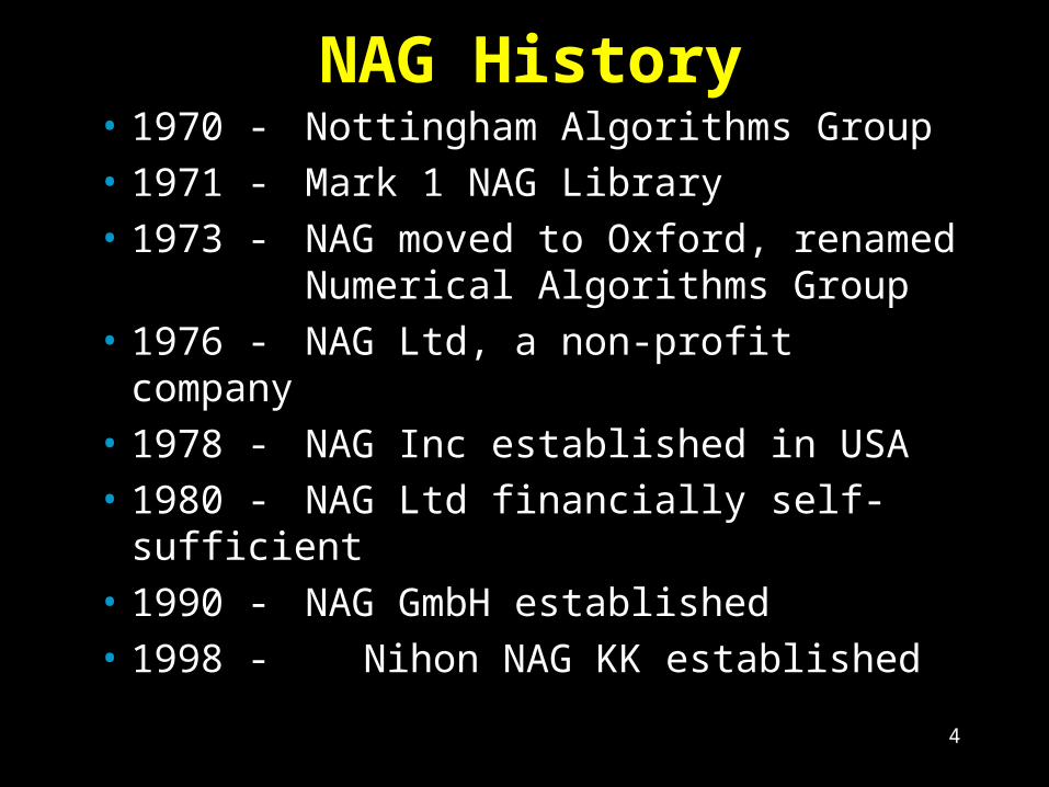
4

NAG History• 1970 - Nottingham Algorithms Group

• 1971 - Mark 1 NAG Library

• 1973 - NAG moved to Oxford, renamed Numerical Algorithms Group

• 1976 - NAG Ltd, a non-profit company

• 1978 - NAG Inc established in USA

• 1980 - NAG Ltd financially self-sufficient

• 1990 - NAG GmbH established

• 1998 - Nihon NAG KK established

5

What does non-profit mean?

No shareholders, no owner

surplus is re-invested in the Company

6

How many people work at NAG?

85 worldwide, 65 in Oxford

12 in Downers Grove

Distributors worldwide

7

NAG Products and Services

• Product Lines– Numerical Libraries– Statistical Systems– NAGWare: Compiler and tools– Visualization and Graphics– PDE Solutions

• Consultancy• Customer Support www.nag.co.uk or www.nag.com

8

NAG Numerical Libraries

F77

F90

C

Parallel

SMP MPI

FL90Plus

9

Quality of Computed Solutions

10

Quality of Computed Solutions

The quality of computed solutions is concerned with assessing how good a computed solution is in some appropriate measure

11

Software Quality

Quality software should implement reliable algorithms and should provide measures of solution quality

12

Floating Point Numbers

Floating point numbers are a subset of the real numbers that can be conveniently represented in the finite word length of a computer, without unduly restricting the range of numbers represented

For example, the IEEE standard uses 64 bits to represent double precision numbers in the approximate range

13

Floating Point Numbers - Representation

14

Floating Point Numbers - Example

15

Floating Point Numbers - Example (cont’d)

0 1 2 3

16

IEEE Arithmetic Standard

ANSI/IEEE Standard 754-1985 is a standard for

binary arithmetic (b = 2). The standard specifies:• Floating point number formats• Results of the basic floating point operations• Rounding modes• Signed zero, infinity ( ) and not-a-number

(NaN)• Floating point exceptions and their handling• Conversion between formats

Most modern machines use IEEE arithmetic.

17

IEEE Arithmetic Formats

Format ecision Exponent Approx Range Approx precision

Single bits 8 bits

Double 53 bits 11 bits

Extended

Pr

24 10 10

10 10

64 15 10 10

38 8

308 16

4932 20

18

Why Worry about Computed Solutions?

• Tacoma bridge collapse• North Sea oil rig collapse• Vancouver stock exchange index, Jan 1982

to Nov 1983• Ariane 5 rocket, flight 501, failure, 4 June

1996• Patriot missile, 25 Feb 1991• Auckland Bridge• London millennium bridge

19

Tacoma Bridge

20

Auckland Bridge, 1975

21

Millennium Bridge, 2000

22

Web Sites

• Disasters attributable to bad numerical computing: http://www.math.psu.edu/dna/disasters/

• Numerical problems: RISKS-LIST: http://catless.ncl.ac.uk/Risks/

• London millennium bridge: http://www.arup.com/MillenniumBridge/

23

Example - Means

Mean of a set of numbers can be outside

their range. Using 3 figure arithmetic:

5.01 5.03 2 10.0 2 5.00

Does this matter? If so, can we guarantee

an answer within range?

24

Example - Sample Variance

22

1

2

2 2

1 1

11

1

1 12

1

For 10000,10001,10002 using 8 figure arithmetic

1 gives: 1.0, 2 gives: 0.0

Are either of these reasonable? (Actually (1) is the

correct ans

n

n ii

n n

n i ii i

T

s x xn

s x xn n

x

wer)

25

Excel Example:Standard Deviation

Microsoft Excel Worksheet

26

Overflow/Underflow Example: Modulus of a Complex Number

2 2

2

1 , where max , , min ,

0 if 0

r i

r i r i

x x x

ba a x x b x x

a

x a

27

Excel Example:Standard Deviation - Overflow

Microsoft Excel Worksheet

28

Stability

The stability of a method for solving a problem is concerned with the sensitivity of the method to (rounding) errors in the solution process

A method that guarantees as accurate a solution as the data warrants is said to be stable, otherwise the method is unstable

29

Condition

The condition of a problem is concerned with the sensitivity of the problem to perturbations in the data

A problem is ill-conditioned if small changes in the data cause relatively large changes in the solution. Otherwise a problem is well-conditioned

30

Condition Examplesx x x

x x x

x x x

x x x

x x x

x x x i

3 2

1 2 3

3 2

1 2 3

3 2

1 2 3

21 120 100 0

1 10

0 99 21 120 99 99 0

1 1117 9 04

101 21 120 100 01 0

1 9 90 104

,

. .

, . , .

. .

, , . .

33

Condition Examples (cont’d)

When

When

I ae be dx

a b

I

a b

I

x x

z( )

,

, .

10

10

1

0

1 101

220

35

Condition Examples (cont’d)

1 2

1 2

1 2

1 2

1 2

1 2

99 98 197

100 99 199

1

98.99 98 197

100 99 199

100, 99

x x

x x

x x

x x

x x

x x

37

Condition Number for Linear Equations

1

1

1

, ( )

( ) , so that

giving

( ) ,

where ( ) is the condition number of

with respect to matrix inversion

Ax b A E x b

A x x Ex x x A Ex

x x EA E A

x A

A A A

A

38

Condition Number Example

1

1 1

1

2 41

99 98, 199

100 99

99 98, 199

100 99

199 4 10

A A

A A

A

39

Stability Examples2

2

1 2

2 1

1.6 100.1 1.251 0

Four significant figure arithmetic on the standard formula

( 4 ) (2 )

gives

62.53, 0.03125,

but using

( )

gives

x x

x b b ac a

x x

x c ax

x

2 0.01251

1 2

Exact solution is

62.55, 0.0125x x

40

Stability Examples (Contd)1

0

1 0

(1 )

Easy to show that

0 1 ( 1)

Integrating by parts gives

1 , 1 1 0.632121

n xn

n

n n

y e x e dx

y n

y ny y e

recursive.m

41

Stability Examples (Contd)

In general

~

~ ~

~ ~

~ ~

~ !

y y

y y y

y y y

y y y

y y nn n

n

0 0

1 0 1

2 1 2

3 2 3

1

1 2 2

1 3 6

1

bg

42

Stability Examples (cont’d)

1

1

1

2 2

1

1

1

In general

1 1 1

n n

n m n m

n m n m

n m

n m n m

m n

n n

y y n

y y

y y n m

y n m

y y n m n m

y y n m n m n

brecursive.m

43

Error Analysis

Error analysis is concerned with establishing whether or not an algorithm is stable for the problem in hand

A forward error analysis is concerned with how close the computed solution is to the exact solution

A backward error analysis is concerned with how well the computed solution satisfies the problem to be solved

Example,

99 98 1 1 , ,

100 99 1 1

2.97Consider

2.99

1.97 0.01 , but

1.99 0.01

1.01Now consider ,

0.99

0.01 , but

01

0.

Ax b r b Ax

A b x

x

x x r

x

x x r

1.97

1.97

45

The Purpose of Error Analysis“The clear identification of the factors determining the stability of an algorithm soon led to the development of better algorithms. The proper understanding of inverse iteration for eigenvectors and the development of the QR algorithm by Francis are the crowning achievements of this line of research.

“For me, then, the primary purpose of the rounding error analysis was insight.”

Wilkinson, 1986Bulletin of the IMA, Vol 22, p197

46

47

Backward Error and Perturbation Analysis

If we know how perturbations in affect the

solution then we can estimate the accuracy of the

computed solution That is, an estimate of the

backward error allows us to estimate the forward error.

Ax b A E x b

A

x

x

x x

xA

E

A

, ~

,~.

~

~

b g

bg

Condition and Error Analysis

forward error

condition number backward error

49

LAPACK

• Systems of linear equations

• Linear least squares problems

• Eigenvalue and singular value problems, including generalized problems

• Matrix factorizations

• Condition and error estimates

• The BLAS as a portability layer

Linear Algebra PACKage for high-performance computers

Dense and banded linear algebra for Shared Memory

LAPACK and Error Bounds

“In Addition to providing faster routines than previously available, LAPACK provides more comprehensive and better error bounds. Our goal is to provide error bounds for most quantities computed by LAPACK.”

LAPACK Users’ Guide, Chapter 4 – Accuracy and Stability

Error Bounds in LAPACK

The Users’ Guide gives details of error bounds and code fragments to compute those bounds. In many cases the routines return the bounds directly

Error Bounds in LAPACK: Example

DGESVX is an 'expert' driver for solving

Estimate of 1/

Estimated forward error for

Componentwise

j

AX B

A

X

DGESVX( ..., RCOND, FERR, BERR, WORK,...)

RCOND -

FERR(j) -

BERR(j) - relative backward error for

(smallest relative change in any element of and

that makes an exact solution)

Reciprocal of pivot growth factor (1/ )

j

j

X

A B

X

WORK(1) -

54

ODE Software Example

NAG routine D02PZF returns global error estimates for the Runge-Kutta solvers D02PCF and D02PDF:

D02PCZ( RMSERR, ERRMAX, TERRMX,…)

RMSERR: Approximate Root mean square error

ERRMAX: Max approximate true error

TERRMX: Point at which max approximate true error occurred

(These routines are based upon RKSUITE)

What to do if Software does not Provide Error Estimates?

• Run the problem with perturbed data

• Better still, use a software tool such as PRECISE which allows you to perform a stochastic analysis

• Put pressure on developers to provide estimates

PRECISE

• Provides a module for statistical backward error analysis

• Provides a module for sensitivity analysis

• http://www.cerfacs.fr/algor/Softs/PRECISE/index.html

Quality of Reliable Software

Chaitin-Chatelin & Frayssé define the quality index

of a reliable algorithm at the computed solution as

( ) ( ) ,

where ( ) is the backward error and is the machine

precision.

(Lecture

x

B xJ x

B x

s on Finite Precision Computations)

58

CADNA

• CADNA is another package with the same aims as PRECISE

http://www-anp.lip6.fr/cadna/Accueil.php

• It is now free to academics

59

Cancellation

4 4

4 4

1.000 1.000 10 1.000 10

1.000 10 1.000 10

0

s

Using four figure decimal arithmetic

60

Interval Analysis

• Interval arithmetic works on intervals that contain the exact solution

• Interval analysis can provide automatic error bounds for a number of problems

• See www.cs.utep.edu/interval-comp/main.html

4 4 4 4

4 4 4 4

1.000 1.000 1.000 10 1.000 10 1.000 10 1.000 10

1.000 10 1.0010 10 1.000 10 1.000 10

0 10

61

Summary• Error analysis gives insight

• In linear algebra we usually aim for a backward error analysis

• Be concerned about the quality of computed solutions

• Use quality software, complain about low quality software

• Write quality software and be proud of your results

62

Quote

“You have been solving these damn problems better than I can pose them.”

Sir Edward Bullard, Director NPL, in a remark to Wilkinson. (mid 1950s.)

See NAG Newsletter 2/83, page 11

References[1] E. Anderson, Z. Bai, C. H. Bischof, J. Demmel, J. J. Dongarra, J. Du Croz, A. Greenbaum, S. Hammarling, A. McKenney, S. Blackford & D. C. Sorensen. LAPACK Users’ Guide, 3rd Edition, SIAM, 1999.

[2] F. Chaitin-Chatelin & V. Frayssé. Lectures on Finite Precision Computations, SIAM, 1996.

[3] G. H. Golub & C. F. Van Loan. Matrix Computations, 3rd Edition, The Johns Hopkins University Press, 1996.

[4] N. J. Higham. Accuracy and Stability of Numerical Algorithms, 2nd edition, SIAM, 2002.

[5] www.cs.utep.edu/interval-comp/main.html

[6] www.nag.co.uk/numeric/numerical_libraries.asp

References (cont’d)[7] F. S. Acton. Numerical Methods that Usually Work. Harper and Row, 1970.

[8] G. E. Forsythe. What is a Satisfactory Quadratic Equation Solver. In Constructive Aspects of the Fundamental Theorem of Algebra, B. Dejon and P. Henrici, P., editors, pages 53-61, Wiley, 1969.

[9] G. E. Forsythe. Pitfalls in Computation, or Why a Math Book isn't enough. Amer. Math. Monthly, 9: 931-995, 1970.

[10] J. H. Wilkinson. The Perfidious Polynomial. In Studies in Numerical Analysis, G. H. Golub, editor, volume 24 of Studies in Mathematics, Mathematical Association of America, Washington D.C., pages 1-24, 1984.