1 : A MATLAB Software for Solving Multiple-Phase … variety of numerical methods and corresponding...
41
1 GPOPS − II: A MATLAB Software for Solving Multiple-Phase Optimal Control Problems Using hp–Adaptive Gaussian Quadrature Collocation Methods and Sparse Nonlinear Programming Michael A. Patterson and Anil V. Rao University of Florida, Gainesville, FL 32611-6250 A general-purpose MATLAB software program called GPOPS - II is described for solving multiple-phase optimal control problems using variable-order Gaussian quadrature collocation methods. The software em- ploys a Legendre-Gauss-Radau quadrature orthogonal collocation method where the continuous-time opti- mal control problem is transcribed to a large sparse nonlinear programming problem (NLP). An adaptive mesh refinement method is implemented that determines the number of mesh intervals and the degree of the approximating polynomial within each mesh interval to achieve a specified accuracy. The software can be interfaced with either quasi-Newton (first derivative) or Newton (second derivative) NLP solvers, and all derivatives required by the NLP solver are approximated using sparse finite-differencing of the optimal control problem functions. The key components of the software are described in detail and the utility of the software is demonstrated on five optimal control problems of varying complexity. The software described in this paper provides researchers a useful platform upon which to solve a wide variety of complex constrained optimal control problems. Categories and Subject Descriptors: G.1.4 [Numerical Analysis]: Optimal Control, Optimization General Terms: Optimal Control, Direct Collocation, Gaussian Quadrature, hp–Adaptive Methods, Numer- ical Methods, MATLAB. Additional Key Words and Phrases: Scientific Computation, Applied Mathematics. ACM Reference Format: Patterson, M. A. and Rao, A. V. 2012. GPOPS-II: A MATLAB Software for Solving Multiple-Phase Optimal Control Problems Using hp–Adaptive Gaussian Quadrature Collocation Methods and Sparse Nonlinear Pro- gramming ACM Trans. Math. Soft. 39, 3, Article 1 (July 2013), 41 pages. DOI = 10.1145/0000000.0000000 http://doi.acm.org/10.1145/0000000.0000000 1. INTRODUCTION Optimal control problems arise in a wide variety of subjects including virtually all branches of engineering, economics, and medicine. Because optimal control applica- tions have increased in complexity in recent years, over the past two decades the subject of optimal control has transitioned from theory to computation. In particu- lar, computational optimal control has become a science in and of itself, resulting in a variety of numerical methods and corresponding software implementations of these methods. The vast majority of software implementations of optimal control today are The authors gratefully acknowledge support for this research from the U.S. Office of Naval Research (ONR) under Grant N00014-11-1-0068 and from the U.S. Defense Advanced Research Projects Agency (DARPA) Under Contract HR0011-12-C-0011. Disclaimer: The views expressed are those of the authors and do not reflect the official policy or position of the Department of Defense or the U.S. Government. Author’s addresses: M. A. Patterson and A. V. Rao, Department of Mechanical and Aerospace Engineering, P.O. Box 116250, University of Florida, Gainesville, FL 32611-6250; e-mail: {mpatterson,anilvrao}@ufl.edu. Permission to make digital or hard copies of part or all of this work for personal or classroom use is granted without fee provided that copies are not made or distributed for profit or commercial advantage and that copies show this notice on the first page or initial screen of a display along with the full citation. Copyrights for components of this work owned by others than ACM must be honored. Abstracting with credit is per- mitted. To copy otherwise, to republish, to post on servers, to redistribute to lists, or to use any component of this work in other works requires prior specific permission and/or a fee. Permissions may be requested from Publications Dept., ACM, Inc., 2 Penn Plaza, Suite 701, New York, NY 10121-0701 USA, fax +1 (212) 869-0481, or [email protected]. © 2013 ACM 1539-9087/2013/07-ART1 $15.00 DOI 10.1145/0000000.0000000 http://doi.acm.org/10.1145/0000000.0000000 ACM Transactions on Mathematical Software, Vol. 39, No. 3, Article 1, Publication date: July 2013.
Transcript of 1 : A MATLAB Software for Solving Multiple-Phase … variety of numerical methods and corresponding...

1
GPOPS− II: A MATLAB Software for Solving Multiple-Phase OptimalControl Problems Using hp–Adaptive Gaussian QuadratureCollocation Methods and Sparse Nonlinear Programming
Michael A. Patterson and Anil V. RaoUniversity of Florida, Gainesville, FL 32611-6250
A general-purpose MATLAB software program called GPOPS− II is described for solving multiple-phaseoptimal control problems using variable-order Gaussian quadrature collocation methods. The software em-ploys a Legendre-Gauss-Radau quadrature orthogonal collocation method where the continuous-time opti-mal control problem is transcribed to a large sparse nonlinear programming problem (NLP). An adaptivemesh refinement method is implemented that determines the number of mesh intervals and the degree ofthe approximating polynomial within each mesh interval to achieve a specified accuracy. The software canbe interfaced with either quasi-Newton (first derivative) or Newton (second derivative) NLP solvers, andall derivatives required by the NLP solver are approximated using sparse finite-differencing of the optimalcontrol problem functions. The key components of the software are described in detail and the utility of thesoftware is demonstrated on five optimal control problems of varying complexity. The software described inthis paper provides researchers a useful platform upon which to solve a wide variety of complex constrainedoptimal control problems.
Categories and Subject Descriptors: G.1.4 [Numerical Analysis]: Optimal Control, Optimization
General Terms: Optimal Control, Direct Collocation, Gaussian Quadrature, hp–Adaptive Methods, Numer-ical Methods, MATLAB.
Additional Key Words and Phrases: Scientific Computation, Applied Mathematics.
ACM Reference Format:
Patterson, M. A. and Rao, A. V. 2012. GPOPS-II: A MATLAB Software for Solving Multiple-Phase OptimalControl Problems Using hp–Adaptive Gaussian Quadrature Collocation Methods and Sparse Nonlinear Pro-gramming ACM Trans. Math. Soft. 39, 3, Article 1 (July 2013), 41 pages.DOI = 10.1145/0000000.0000000 http://doi.acm.org/10.1145/0000000.0000000
1. INTRODUCTION
Optimal control problems arise in a wide variety of subjects including virtually allbranches of engineering, economics, and medicine. Because optimal control applica-tions have increased in complexity in recent years, over the past two decades thesubject of optimal control has transitioned from theory to computation. In particu-lar, computational optimal control has become a science in and of itself, resulting ina variety of numerical methods and corresponding software implementations of thesemethods. The vast majority of software implementations of optimal control today are
The authors gratefully acknowledge support for this research from the U.S. Office of Naval Research (ONR)under Grant N00014-11-1-0068 and from the U.S. Defense Advanced Research Projects Agency (DARPA)Under Contract HR0011-12-C-0011. Disclaimer: The views expressed are those of the authors and do notreflect the official policy or position of the Department of Defense or the U.S. Government.Author’s addresses: M. A. Patterson and A. V. Rao, Department of Mechanical and Aerospace Engineering,P.O. Box 116250, University of Florida, Gainesville, FL 32611-6250; e-mail: mpatterson,[email protected] to make digital or hard copies of part or all of this work for personal or classroom use is grantedwithout fee provided that copies are not made or distributed for profit or commercial advantage and thatcopies show this notice on the first page or initial screen of a display along with the full citation. Copyrightsfor components of this work owned by others than ACM must be honored. Abstracting with credit is per-mitted. To copy otherwise, to republish, to post on servers, to redistribute to lists, or to use any componentof this work in other works requires prior specific permission and/or a fee. Permissions may be requestedfrom Publications Dept., ACM, Inc., 2 Penn Plaza, Suite 701, New York, NY 10121-0701 USA, fax +1 (212)869-0481, or [email protected].© 2013 ACM 1539-9087/2013/07-ART1 $15.00DOI 10.1145/0000000.0000000 http://doi.acm.org/10.1145/0000000.0000000
ACM Transactions on Mathematical Software, Vol. 39, No. 3, Article 1, Publication date: July 2013.

1:2 M. A. Patterson and A. V. Rao
those that involve the direct transcription of a continuous-time optimal control prob-lem to a nonlinear programming problem (NLP), and the NLP is solved using wellestablished techniques. Examples of well known software for solving optimal controlproblems include SOCS [Betts 1998], DIRCOL [von Stryk 2000], GESOP [Jansch et al.1994], OTIS [Vlases et al. 1990], MISER [Goh and Teo 1988], PSOPT [Becerra 2009],GPOPS [Rao et al. 2010], ICLOCS [Falugi et al. 2010], JModelica [Åkesson et al. 2010],ACADO [Houska et al. 2011], and Sparse Optimization Suite (SOS) [Betts 2013].
Over the past two decades, direct collocation methods have become popular inthe numerical solution of nonlinear optimal control problems. In a direct collocationmethod, the state and control are discretized at a set of appropriately chosen pointsin the time interval of interest. The continuous-time optimal control problem is thentranscribed to a finite-dimensional NLP. The resulting NLP is then solved using wellknown software such as SNOPT [Gill et al. 2002], IPOPT [Wächter and Biegler 2006;Biegler and Zavala 2008] and KNITRO [Byrd et al. 2006]. Originally, direct collocationmethods were developed as h methods (for example, Euler or Runge-Kutta methods)where the time interval is divided into a mesh and the state is approximated usingthe same fixed-degree polynomial in each mesh interval. Convergence in an h methodis then achieved by increasing the number and placement of the mesh points [Betts2010; Jain and Tsiotras 2008; Zhao and Tsiotras 2011]. More recently, a great deal ofresearch as been done in the class of direct Gaussian quadrature orthogonal colloca-tion methods [Elnagar et al. 1995; Elnagar and Razzaghi 1998; Benson et al. 2006;Huntington et al. 2007; Huntington and Rao 2008; Gong et al. 2008b; Rao et al. 2010;Garg et al. 2010; Garg et al. 2011a; Garg et al. 2011b; Kameswaran and Biegler 2008;Darby et al. 2011a; Patterson and Rao 2012]. In a Gaussian quadrature collocationmethod, the state is typically approximated using a Lagrange polynomial where thesupport points of the Lagrange polynomial are chosen to be points associated with aGaussian quadrature. Originally, Gaussian quadrature collocation methods were im-plemented as p methods using a single interval. Convergence of the p method wasthen achieved by increasing the degree of the polynomial approximation. For problemswhose solutions are smooth and well-behaved, a p Gaussian quadrature collocationmethod has a simple structure and converges at an exponential rate [Canuto et al.1988; Fornberg 1998; Trefethen 2000]. The most well developed p Gaussian quadra-ture methods are those that employ either Legendre-Gauss (LG) points [Benson et al.2006; Rao et al. 2010], Legendre-Gauss-Radau (LGR) points [Kameswaran and Biegler2008; Garg et al. 2010; Garg et al. 2011a], or Legendre-Gauss-Lobatto (LGL) points[Elnagar et al. 1995].
In this paper we describe a new optimal control software called GPOPS− II that em-ploys hp-adaptive Gaussian quadrature collocation methods. An hp-adaptive methodis a hybrid between a p method and an h method in that both the number of meshintervals and the degree of the approximating polynomial within each mesh intervalcan be varied in order to achieve a specified accuracy in the numerical approxima-tion of the solution to the continuous-time optimal control problem. As a result, in anhp-adaptive method it is possible to take advantage of the exponential convergenceof a global Gaussian quadrature method in regions where the solution is smooth andintroduce mesh points only near potential discontinuities or in regions where the solu-tion changes rapidly. Originally, hp methods were developed as finite-element methodsfor solving partial differential equations [Babuska et al. 1986; Babuska and Rhein-boldt 1982; 1979; 1981]. In the past few years the problem of developing hp methodsfor solving optimal control problems has been of interest [Darby et al. 2011b; 2011c].The work of [Darby et al. 2011b; 2011c] provides examples of the benefits of using anhp–adaptive method over either a p method or an h method. This recent research has
ACM Transactions on Mathematical Software, Vol. 39, No. 3, Article 1, Publication date: July 2013.

GPOPS− II: An hp Gaussian Quadrature MATLAB Optimal Control Software 1:3
shown that convergence using hp methods can be achieved with a significantly smallerfinite-dimensional approximation than would be required when using either an h or ap method.
It is noted that previously the software GPOPS was published in Rao et al. [2010].While GPOPS is similar to GPOPS− II in that both software programs implementGaussian quadrature collocation, GPOPS− II is a fundamentally different softwareprogram from GPOPS. First, GPOPS employs p (global) collocation in each phase ofthe optimal control problem. It is known that p collocation schemes are limited in thatthey have difficulty solving problems whose solutions change rapidly in certain re-gions or are discontinuous. Moreover, p methods become computationally intractableas the degree of the approximating polynomial becomes very large. GPOPS− II, how-ever, employs hp-adaptive mesh refinement where the polynomial degree, number ofmesh intervals, and width of each mesh interval can be varied. The hp-adaptive meth-ods allow for placement of collocation points in regions of the solution where additionalinformation is needed to capture key features of the optimal solution. Next, GPOPS islimited in that it can be used with only quasi-Newton (first derivative) NLP solvers andderivative approximations were performed on high dimensional NLP functions. On theother hand, GPOPS− II implements sparse derivative approximations by approximat-ing derivatives of the optimal control functions and inserting these derivatives into theappropriate locations in the NLP derivative functions. Moreover, GPOPS− II imple-ments approximations to both first and second derivatives. Consequently, GPOPS− II
utilizes in an efficient manner the full capabilities of a much wider range of NLPsolvers (for example, full Newton NLP solvers such as IPOPT [Biegler and Zavala2008] and KNITRO [Byrd et al. 2006]) and, as a result, is capable of solving a muchwider range of optimal control problems as compared with GPOPS.
The objective of this paper is to provide researchers with a novel efficient general-purpose optimal control software that is capable of solving a wide variety of complexconstrained continuous-time optimal control problems. In particular, the software de-scribed in this paper employs a differential and implicit integral form of the multiple-interval version of the Legendre-Gauss-Radau (LGR) collocation method [Garg et al.2010; Garg et al. 2011a; Garg et al. 2011b; Patterson and Rao 2012]. The LGR colloca-tion method is chosen for use in the software because it provides highly accurate state,control, and costate approximations while maintaining a relatively low-dimensionalapproximation of the continuous-time problem. The key components of the softwareare then described, and the software is demonstrated on five examples from the openliterature that have been studied extensively and whose solutions are known. Each ofthese examples demonstrates different capabilities of the software. The first exampleis the hyper-sensitive optimal control problem from Rao and Mease [2000] and demon-strates the ability of the software to accurately solve a problem whose optimal solu-tion changes rapidly in particular regions of the solution. The second example is thereusable launch vehicle entry problem taken from Betts [2010] and demonstrates theability of GPOPS− II to compute an accurate solution using a relatively coarse mesh.The third example is a space station attitude control problem taken from Pietz [2003]and Betts [2010] and demonstrates the ability of the software to generate accuratesolutions to a problem whose solution is not intuitive. The fourth example is a chemi-cal kinetic batch reactor problem taken from Leineweber [1998] and Betts [2010] andshows the ability of the software to handle a multiple-phase optimal control problemthat is badly scaled. The fifth example is a launch vehicle ascent problem taken fromBenson [2004], Rao et al. [2010], and Betts [2010] that again demonstrates the abilityof the software to solve a multiple-phase optimal control problem. In order to validatethe results, the solutions obtained using GPOPS− II are compared against the solu-
ACM Transactions on Mathematical Software, Vol. 39, No. 3, Article 1, Publication date: July 2013.

1:4 M. A. Patterson and A. V. Rao
tions obtained using the software Sparse Optimization Suite (SOS) [Betts 2013] whereSOS is based on the collection of algorithms developed in Betts [2010].
This paper is organized as follows. In Section 2 we describe a general multiple-phaseoptimal control problem. In Section 3 we describe the Radau collocation method thatis used as the basis of GPOPS− II. In Section 4 we describe the key components ofGPOPS− II. In Section 5 we show the results obtained using the software on the fiveaforementioned examples. In Section 6 we provide a discussion of the results obtainedusing the software. In Section 7 we discuss possible limitations of the software. Finally,in Section 8 we provide conclusions on our work.
2. GENERAL MULTIPLE-PHASE OPTIMAL CONTROL PROBLEMS
The general multiple-phase optimal control problem that can be solved by GPOPS− II
is given as follows. First, let p ∈ [1, . . . , P ] be the phase number where P as the to-tal number of phases. The optimal control problem is to determine the state, y(p)(t) ∈
Rn(p)y , control, u(p)(t) ∈ R
n(p)u , integrals, q(p) ∈ R
n(p)q , start times, t(p)0 ∈ R, phase ter-
minus times, t(p)f ∈ R, in all phases p ∈ [1, . . . , P ], along with the static parameterss ∈ R
ns , that minimize the objective functional
J = φ(
e(1), . . . , e(P ), s)
, (1)
subject to the dynamic constraints
y(p) = a(p)(y(p),u(p), t(p), s), (p = 1, . . . , P ), (2)
the event constraints
bmin ≤ b(
e(1), . . . , e(P ), s)
≤ bmax, (3)
where e(p) =[
y(p)(t(p)0 ), t
(p)0 ,y(p)(t
(p)f ), t
(p)f ,q(p)
]
, (p = 1, . . . , P ), the inequality path
constraints
c(p)min ≤ c(p)(y(p),u(p), t(p), s) ≤ c(p)max, (p = 1, . . . , P ), (4)
the static parameter constraints
smin ≤ s ≤ smax, (5)
and the integral constraints
q(p)min ≤ q(p) ≤ q(p)
max, (p = 1, . . . , P ), (6)
where
e(p) =[
y(p)(
t(p)0
)
, t(p)0 ,y(p)
(
t(p)f
)
, t(p)f ,q(p)
]
, (p = 1, . . . , P ), (7)
and the integrals in each phase are defined as
q(p)i =
∫ t(p)f
t(p)0
g(p)i (y(p),u(p), t(p), s)dt, (i = 1, . . . n(p)q ), (p = 1, . . . , P ). (8)
It is important to note that the event constraints of Eq. (3) can contain any functionsthat relate information at the start and/or terminus of any phase (including relation-ships that include both static parameters and integrals) and that the phases them-selves need not be sequential. It is noted that the approach to linking phases is basedon well-known formulations in the literature such as those given in Ref. Betts [1990]and Betts [2010]. A schematic of how phases can potentially be linked is given in Fig. 1.
ACM Transactions on Mathematical Software, Vol. 39, No. 3, Article 1, Publication date: July 2013.

GPOPS− II: An hp Gaussian Quadrature MATLAB Optimal Control Software 1:5
Phase 1 Phase 2 Phase 3
Phase 5
Phase 4
Tra
ject
ory
time
Phases 1 and 2 Connected
Phases 2 and 3 ConnectedPhases 2 and 5 Connected
Phases 3 and 4 Connected
Fig. 1: Schematic of linkages for multiple-phase optimal control problem. The exampleshown in the picture consists of five phases where the ends of phases 1, 2, and 3 arelinked to the starts of phases 2, 3, and 4, respectively, while the end of phase 2 is linkedto the start of phase 5.
3. MULTIPLE-INTERVAL RADAU COLLOCATION METHOD
In this section we describe the multiple-interval Radau collocation method [Garg et al.2010; Garg et al. 2011a; Garg et al. 2011b; Patterson and Rao 2012] that forms the ba-sis for GPOPS− II. In order to make the description of the Radau collocation methodas clear as possible, in this section we consider only a one-phase optimal control prob-lem. After formulating the one-phase optimal control problem we develop the Radaucollocation method itself.
3.1. Single-Phase Optimal Control Problem
In order to describe the hp Radau method that is implemented in the software, it willbe useful to simplify the general optimal control problem given in Eqs. (1)–(8) to a one-phase problem as follows. Determine the state, y(t) ∈ R
ny , the control, u(t) ∈ Rnu , the
integrals, q ∈ Rnq , the initial time, t0, and the terminal time tf on the time interval
t ∈ [t0, tf ] that minimize the cost functional
J = φ(y(t0), t0,y(tf ), tf ,q) (9)
subject to the dynamic constraints
dy
dt= a(y(t),u(t), t), (10)
the inequality path constraints
cmin ≤ c(y(t),u(t), t) ≤ cmax, (11)
the integral constraints
qi =
∫ tf
t0
gi(y(t),u(t), t) dt, (i = 1, . . . , nq), (12)
ACM Transactions on Mathematical Software, Vol. 39, No. 3, Article 1, Publication date: July 2013.

1:6 M. A. Patterson and A. V. Rao
and the event constraints
bmin ≤ b(y(t0), t0,y(tf ), tf ,q) ≤ bmin. (13)
The functions φ, q, a, c and b are defined by the following mappings:
φ : Rny × R× R
ny × R× Rnq → R,
q : Rny × R
nu × R → Rnq ,
a : Rny × R
nu × R → Rny ,
c : Rny × R
nu × R → Rnc ,
b : Rny × R× R
ny × R× Rnq → R
nb ,
where we remind the reader that all vector functions of time are treated as row vectors.In order to employ the hp Radau collocation method used in GPOPS− II, the continu-
ous optimal control problem of Eqs. (9)–(13) is modified as follows. First, let τ ∈ [−1,+1]be a new independent variable. The variable t is then defined in terms of τ as
t =tf − t0
2τ +
tf + t02
. (14)
The optimal control problem of Eqs. (9)–(13) is then defined in terms of the variableτ as follows. Determine the state, y(τ) ∈ R
ny , the control u(τ) ∈ Rnu , the integral
q ∈ Rnq , the initial time, t0, and the terminal time tf on the time interval τ ∈ [−1,+1]
that minimize the cost functional
J = φ(y(−1), t0,y(+1), tf ,q) (15)
subject to the dynamic constraints
dy
dτ=tf − t0
2a(y(τ),u(τ), τ ; t0, tf ), (16)
the inequality path constraints
cmin ≤ c(y(τ),u(τ), τ ; t0, tf ) ≤ cmax, (17)
the integral constraints
qi =tf − t0
2
∫ +1
−1
gi(y(τ),u(τ), τ ; t0, tf ) dτ, (i = 1, . . . , nq), (18)
and the event constraints
bmin ≤ b(y(−1), t0,y(+1), tf ,q) ≤ bmin. (19)
Suppose now that the interval τ ∈ [−1,+1] is divided into a mesh consisting of Kmesh intervals [Tk−1, Tk], k = 1, . . . ,K, where (T0, . . . , TK) are the mesh points. Themesh points have the property that −1 = T0 < T1 < T2 < · · · < TK = Tf = +1.Next, let y(k)(τ) and u(k)(τ) be the state and control in mesh interval k. The optimalcontrol problem of Eqs. (15)–(19) can then written as follows. First, the cost functionalof Eq. (15) can be written as
J = φ(y(1)(−1), t0,y(K)(+1), tf ,q), (20)
Next, the dynamic constraints of Eq. (16) in mesh interval k can be written as
dy(k)(τ (k))
dτ (k)=tf − t0
2a(y(k)(τ (k)),u(k)(τ (k)), τ (k); t0, tf ), (k = 1, . . . ,K). (21)
Furthermore, the path constraints of (17) in mesh interval k are given as
cmin ≤ c(y(k)(τ (k)),u(k)(τ (k)), τ (k); t0, tf ) ≤ cmax, (k = 1, . . . ,K). (22)
ACM Transactions on Mathematical Software, Vol. 39, No. 3, Article 1, Publication date: July 2013.

GPOPS− II: An hp Gaussian Quadrature MATLAB Optimal Control Software 1:7
the integral constraints of (18) are given as
qj =tf − t0
2
K∑
k=1
∫ Tk
Tk−1
gj(y(k)(τ (k)),u(k)(τ (k)), τ (k); t0, tf ) dτ, (j = 1, . . . , nq, k = 1 . . . ,K).
(23)Finally, the event constraints of Eq. (19) are given as
bmin ≤ b(y(1)(−1), t0,y(K)(+1), tf ,q) ≤ bmax. (24)
Because the state must be continuous at each interior mesh point, it is requiredthat the condition y(k)(Tk) = y(k+1)(Tk) be satisfied at the interior mesh points(T1, . . . , TK−1).
3.2. Approximation of the Optimal Control Problem via Radau Collocation Method
The method utilized in the software is an implementation of the previously developedmultiple-interval Legendre-Gauss-Radau quadrature orthogonal collocation method(known hereafter as the Radau collocation method) [Garg et al. 2010; Garg et al. 2011a;Garg et al. 2011b; Patterson and Rao 2012]. In the Radau collocation method, the stateof the continuous-time optimal control problem is approximated in each mesh intervalk ∈ [1, . . . ,K] as
y(k)(τ) ≈ Y(k)(τ) =
Nk+1∑
j=1
Y(k)j ℓ
(k)j (τ), ℓ
(k)j (τ) =
Nk+1∏
l=1
l 6=j
τ − τ(k)l
τ(k)j − τ
(k)l
, (25)
where τ ∈ [−1,+1], ℓ(k)j (τ), j = 1, . . . , Nk + 1, is a basis of Lagrange polynomials,
(τ(k)1 , . . . , τ
(k)Nk
) are the Legendre-Gauss-Radau [Abramowitz and Stegun 1965] (LGR)collocation points in mesh interval k defined on the subinterval τ (k) ∈ [Tk−1, Tk), andτ(k)Nk+1 = Tk is a noncollocated point. Differentiating Y(k)(τ) in Eq. (25) with respect toτ , we obtain
dY(k)(τ)
dτ=
Nk+1∑
j=1
Y(k)j
dℓ(k)j (τ)
dτ. (26)
The cost functional of Eq. (20) is then shown as
J = φ(Y(1)1 , t0,Y
(K)NK+1, tf ,q), (27)
where Y(1)1 is the approximation of y(T0 = −1), and Y
(K)NK+1 is the approximation of
y(TK = +1). Collocating the dynamics of Eq. (21) at the Nk LGR points using Eq. (26),we have
Nk+1∑
j=1
D(k)ij Y
(k)j −
tf − t02
a(Y(k)i ,U
(k)i , τ
(k)i ; t0, tf ) = 0, (i = 1, . . . , Nk). (28)
where U(k)i , i = 1, . . . , Nk, are the approximations of the control at the Nk LGR points
in mesh interval k ∈ [1, . . . ,K], and t(k)i are obtained from τ(k)k using Eq. (14) and
D(k)ij =
[
dℓ(k)j (τ)
dτ
]
τ(k)i
, (i = 1, . . . , Nk, j = 1, . . . , Nk + 1, k = 1, . . . ,K), (29)
ACM Transactions on Mathematical Software, Vol. 39, No. 3, Article 1, Publication date: July 2013.

1:8 M. A. Patterson and A. V. Rao
is the Nk × (Nk + 1) Legendre-Gauss-Radau differentiation matrix [Garg et al. 2010]in mesh interval k ∈ [1, . . . ,K]. While the dynamics can be collocated in differentialform, an alternative approach is to collocate the dynamics using the equivalent implicitintegral form of the Radau collocation method as described in Garg et al. [2010; Garget al. [2011a; Garg et al. [2011b]. Collocating the dynamics using the implicit integralform of the Radau collocation method we have
Y(k)i+1 −Y
(k)1 −
tf − t02
Nk∑
j=1
I(k)ij a(Y
(k)i ,U
(k)i , τ
(k)i ; t0, tf ) = 0, (i = 1, . . . , Nk), (30)
where I(k)ij , (i = 1, . . . , Nk, j = 1, . . . , Nk, k = 1, . . . ,K) is the Nk × Nk Legendre-Gauss-
Radau integration matrix in mesh interval k ∈ [1, . . . ,K], and is obtained from thedifferentiation matrix as [Garg et al. 2010; Garg et al. 2011a; Garg et al. 2011b]
I(k) ≡[
D(k)2:Nk+1
]−1
,
Finally, it is noted for completeness that I(k)D(k)1 = −1, where 1 is a column vector of
length Nk of all ones. It is noted that Eqs. (28) and (30) can be be evaluated over allintervals simultaneously using the composite Legendre-Gauss-Radau differentiationmatrix D, and the composite Legendre-Gauss-Radau integration matrix I respectively.Furthermore, the sparse structure of the composite Legendre-Gauss-Radau differen-tiation matrix D can be seen in Fig. 2, and the structure of the composite Legendre-Gauss-Radau integration matrix I can be seen in Fig. 3. Next, the path constraints ofEq. (22) in mesh interval k ∈ [1, . . . ,K] are enforced at the Nk LGR points as
cmin ≤ c(Y(k)i ,U
(k)i , τ
(k)i ; t0, tf ) ≤ cmax, (i = 1, . . . , Nk), (31)
the integral constraints of Eq. (23) is then approximated as
qj ≈K∑
k=1
Nk∑
i=1
tf − t02
w(k)i gj(Y
(k)i ,U
(k)i , τ
(k)i ; t0, tf ), (i = 1, . . . , Nk, j = 1, . . . , nq), (32)
where w(k)j , j = 1, . . . , Nk are the LGR quadrature weights [Abramowitz and Stegun
1965] in mesh interval k ∈ [1, . . . ,K] defined on the interval τ ∈ [τk−1, τk). Further-more, the event constraints of Eq. (24) are approximated as
bmin ≤ b(Y(1)1 , t0,Y
(K)NK+1, tf ,q) ≤ bmax. (33)
It is noted that continuity in the state at the interior mesh points k ∈ [1, . . . ,K − 1] isenforced via the condition
Y(k)Nk+1 = Y
(k+1)1 , (k = 1, . . . ,K − 1), (34)
where we note that the same variable is used for both Y(k)Nk+1 and Y
(k+1)1 in the soft-
ware implementation. Hence, the constraint of Eq. (34) is eliminated from the problembecause it is taken into account explicitly. The NLP that arises from the Radau collo-cation method is then to minimize the cost function of Eq. (27) subject to the algebraicconstraints of Eqs. (28)–(33).
4. MAJOR COMPONENTS OF GPOPS− II
In this section we describe the major components of the MATLAB software GPOPS− II
that implements the aforementioned Radau collocation method. In Section 4.1 we de-scribe the large sparse nonlinear programming problem (NLP) associated with the
ACM Transactions on Mathematical Software, Vol. 39, No. 3, Article 1, Publication date: July 2013.

GPOPS− II: An hp Gaussian Quadrature MATLAB Optimal Control Software 1:9
Block 1
Block 2
Block 3
Block K
(2) Zeros Except in Blocks
(1) Block k is of Size Nk by Nk+1
(3) Total Size N by N+1
Fig. 2: Structure of Composite Legendre-Gauss-Radau Differentiation Matrix Wherethe Mesh Consists of K Mesh Intervals.
Block 1
Block 2
Block 3
Block K
(2) Zeros Except in Blocks
(1) Block k is of Size Nk by Nk
(3) Total Size N by N
Fig. 3: Structure of Composite Legendre-Gauss-Radau Integration Matrix Where theMesh Consists of K Mesh Intervals.
Radau collocation method. In Section 4.2 we show the structure of the NLP describedin Section 4.1. In Section 4.3 we describe the method for scaling the NLP via scalingof the optimal control problem. In Section 4.4 we describe the approach for estimatingthe derivatives required by the NLP solver. In Section 4.5 we describe the method fordetermining the dependencies of each optimal control function in order to provide themost sparse NLP to the NLP solver. In Section 4.6 we describe the hp-adaptive meshrefinement methods that are included in the software in order to iterative determine amesh that meets a user-specified accuracy tolerance. Finally, in Section 4.7 we providea high level description of the algorithmic flow of GPOPS− II.
4.1. Sparse NLP Arising from Multiple-Interval Radau Collocation Method
The nonlinear programming problem (NLP) associated with the hp Radau discretizedscaled continuous-time optimal control problem is given as follows. Determine the de-cision vector Z that minimizes the objective function
Φ(Z) (35)
ACM Transactions on Mathematical Software, Vol. 39, No. 3, Article 1, Publication date: July 2013.

1:10 M. A. Patterson and A. V. Rao
subject to the constraints
Fmin ≤ F(Z) ≤ Fmax. (36)
and the variable bounds
Zmin ≤ Z ≤ Zmax. (37)
It is noted that the size of the NLP arising from the hp Radau collocation methodchanges depending upon the number of mesh intervals and LGR points used in eachphase to discretize the continuous-time optimal control problem, but the structure ofthe NLP is the same regardless of the number of mesh intervals or number of LGRpoints used in the discretization.
4.1.1. NLP Variables. The NLP decision vector Z is given as
Z =
z(1)
...z(P )
s1...sns
, (38)
where z(p) contains all the variables of phase p = 1 . . . P , and si (i = 1, . . . , ns) are thestatic parameters in the problem. The phase-dependent variables of Eq. (38) z(p) (p =1, . . . , P ), are given as
z(p) =
V(p)1...
V(p)
n(p)y
W(p)1...
W(p)
n(p)u
q(p)
t(p)0
t(p)f
, (p = 1, . . . , P ), (39)
where V(p)i ∈ R
(N(p)+1) (i = 1, . . . , n(p)y ) is the ith column of the matrix
V(p) =
Y(p)1...
Y(p)
N(p)+1
∈ R(N(p)+1)×n(p)
y , (40)
W(p)i ∈ R
N(p)
(i = 1, . . . , n(p)u ) is the ith column of the matrix,
W(p) =
U(p)1...
U(p)
N(p)
∈ R
N(p)×n(p)u , (41)
ACM Transactions on Mathematical Software, Vol. 39, No. 3, Article 1, Publication date: July 2013.

GPOPS− II: An hp Gaussian Quadrature MATLAB Optimal Control Software 1:11
q(p) is a column vector containing the n(p)q integral constraint variables, and t(p)0 ∈ R
and t(p)f ∈ R are scalars corresponding to the initial and terminal times in phase p ∈
[1, . . . , P ]. We remind the reader again that because the state and control are beingtreated as row vectors, the ith row in the matrices of Eqs. (40) and (40) corresponds tothe value of the discretized state and control at the time τ (p)i . Finally, the bounds Zmin
and Zmax are defined from the optimal control variable bounds as supplied by the user.
4.1.2. NLP Objective and Constraint Functions. The NLP objective function Φ(Z) is definedas follows
Φ(Z) = φ (42)
where φ is the optimal control objective function evaluated at the discrete variables de-fined in function of Eq. (1). The NLP constraint function vector F(Z) is then assembledas
F =
f (1)
...f (P )
b
, (43)
where f (p) are the constraints in phase p ∈ [1, . . . , P ] and b is the vector of n(p)b eventconstraints evaluated at the discrete variables defined in function of Eq. (3). Thephase-dependent constraints of Eq. (43) f (p) (p ∈ [1, . . . , P ] have the structure
f (p) =
∆(p)1...
∆(p)
n(p)y
C(p)1...
C(p)
n(p)c
ρ(p)
, (p = 1, . . . , P ), (44)
where ∆(p)i ∈ R
N(p)
(i = 1, . . . , n(p)y ) is the ith column in the defect constraint matrix
that results from either the differential or implicit integral form of the Radau colloca-tion method. The defect matrix that results from the differential form is defined as
∆(p) = D(p)Y(p) −t(p)f − t
(p)0
2A(p) ∈ R
N(p)×n(p)y . (45)
The defect matrix that results from the implicit integral form is defined as
∆(p) = E(p)Y(p) −t(p)f − t
(p)0
2I(p)A(p) ∈ R
N(p)×n(p)y , (46)
where the matrix A is the right hand side of the dynamics evaluated at each collocationpoint
A(p) =
a(Y(p)1 ,U
(p)1 , t
(p)1 , s)
...a(Y
(p)
N(p) ,U(p)
N(p) , t(p)
N(p) , s)
∈ R
N(p)×n(p)y , (47)
ACM Transactions on Mathematical Software, Vol. 39, No. 3, Article 1, Publication date: July 2013.

1:12 M. A. Patterson and A. V. Rao
Block 1
Block 2
Block 3
Block K
(3) Zeros Except in Blocks
(1) Block k is of Size Nk by Nk+1
(4) Total Size N by N+1
-1
-1
-1
-1
-1
1
1
1
1
1
-1
-1
-1
-1
-1
1
1
1
1
1
-1
-1
-1
1
1
1
-1
-1
-1
-1
1
1
1
1
Fig. 4: Matrix E Corresponding to the Defect Constraints of Eq. (46) for One Phase ofa P -Phase Optimal Control Problem Discretized Using the Radau Collocation Method.
E(p) is an N (p)× (N (p)+1) matrix that is used to compute the difference Y(p,k)i+1 −Y
(p,k)1
for each interval k = 1, . . . ,K(p), and each phase p = 1, . . . , P and has the structureshown in Fig. 4, C(p)
i ∈ RN(p)
, (i = 1, . . . , n(p)c ), is the ith column of the path constraint
matrix
C(p) =
c(Y(p)1 ,U
(p)1 , t
(p)1 , s)
...c(Y
(p)
N(p) ,U(p)
N(p) , t(p)
N(p) , s)
∈ R
N(p)×n(p)c , (48)
ρ(p) is a vector of length n
(p)
q(p)where the ith element of ρ(p) is given as
ρ(p)i = q
(p)i −
t(p)f − t
(p)0
2
[
w(p)]T
G(p)i , (i = 1, . . . , n(p)q ), (49)
where G(p)i ∈ R
N(p)
(i = 1, . . . , n(p)q ) is the ith column of the integrand matrix
G(p) =
g(Y(p)1 ,U
(p)1 , t
(p)1 , s)
...g(Y
(p)
N(p) ,U(p)
N(p) , t(p)
N(p) , s)
∈ R
N(p)×n(p)q . (50)
It is noted that the defect and integral constraints are all equality constraints of theform
∆(p) = 0,ρ(p) = 0,
(51)
while the discretized path constraints and boundary conditions are inequality con-straints of the form
C(p)min ≤ C(p) ≤ C
(p)max,
bmin ≤ b ≤ bmax.(52)
4.2. Sparse Structure of NLP Derivative Functions
The structure of the NLP created by the Radau collocation method has been describedin detail in Patterson and Rao [2012]. Figures 5 and 6 show the structure of the NLP
ACM Transactions on Mathematical Software, Vol. 39, No. 3, Article 1, Publication date: July 2013.

GPOPS− II: An hp Gaussian Quadrature MATLAB Optimal Control Software 1:13
constraint Jacobian and Lagrangian Hessian for a single-phase optimal control prob-lem using the differential and integral forms of the Radau method. For a multiple-phase optimal control problem, the constraint Jacobian structure in either the differ-ential or integral form is a block-diagonal version of the single-phase NLP constraintJacobian where, excluding the event constraints and the static parameters, each blockhas the structure as seen in either Fig. 5a or 6a. The derivatives of the event con-straints are located in the final rows of the constraint Jacobian, while the derivativesof all functions with respect to the static parameters are located in the final columns ofthe constraint Jacobian. Similarly, the multiple-phase NLP Lagrangian Hessian usingeither the differential or integral form of the Radau method consists of a block-diagonalversion of the single-phase NLP Lagrangian Hessian where, excluding the static pa-rameters, each block has the structure seen in either Fig. 5b or 6b, with additionalnonzero elements arising from the second derivatives of the event constraints, b, andthe objective function, φ. The second derivatives of the Lagrangian with respect to thestatic parameters appear in the final rows and columns of the Lagrangian Hessian.For more details details on the sparse structure of the NLP arising from the multiple-phase Radau collocation method, please see Patterson and Rao [2012].
4.3. Optimal Control Problem Scaling for NLP
The NLP described in Section 4.1 must be well scaled (that is, the variables and con-straints should each be as close as possible O(1) as described in Gill et al. [1981]) inorder for the NLP solver to obtain a solution. GPOPS− II includes the option for theNLP to be scaled automatically by scaling the continuous-time optimal control prob-lem. The approach to automatic scaling is to scale the variables and the first deriva-tives of the optimal control functions to be ≈ O(1). First, the optimal control variablesare scaled to lie on the unit interval [−1/2, 1/2] and is accomplished as follows. Supposeit is desired to scale an arbitrary variable x ∈ [a, b] to x such that x ∈ [−1/2, 1/2]. Thisvariable scaling is accomplished via the affine transformation
x = vxx+ rx, (53)
where vx and rx are the variable scale and shift, respectively, defined as
vx =1
b− a,
rx =1
2−
b
b− a.
(54)
Every variable in the continuous-time optimal control problem is scaled using Eqs. (53)and (54). Next, the Jacobian of the NLP constraints can be made approximately O(1)by scaling the derivatives of the optimal control functions to be approximately unity.First, using the approach derived in [Betts 2010], in GPOPS− II the defect constraintsare scaled using the same scale factors as was used to scale the state. Next, the objec-tive function, event constraint, and path constraint scale factors are obtained as theaverage norm of each gradient across a variety of sample points within the bounds ofthe unscaled optimal control problem, where the scale factor is the reciprocal of theappropriate average norm.
4.4. Computation of Derivatives Required by the NLP Solver
The optimal control problem derivative functions are obtained by exploiting the sparsestructure of the NLP arising from the hp Radau collocation method. Specifically, in Pat-terson and Rao [2012] it has been shown that using either the derivative or integralform of the Radau collocation method the NLP derivatives can be obtained by com-puting the derivatives of the optimal control problem functions at the LGR points and
ACM Transactions on Mathematical Software, Vol. 39, No. 3, Article 1, Publication date: July 2013.

1:14 M. A. Patterson and A. V. Rao
Def
ect
1
State 1 State 2 State ny
Either Zeros or
Diagonal Block
Either Zeros or
Diagonal Block
Either Zeros or
Diagonal Block
Zeros or Diagonal
Block+D-M
atrix Zeros or D
iagonal
Block+D-M
atrix
Def
ect
2D
efec
t n
y
Control 1 Control nu
Pat
h 1
Either Zeros or
Diagonal Block
Pat
h n
c
Either Zeros or
Diagonal Block
Either Zeros or
Diagonal Block
Ev
ent
Co
nst
rain
ts
Either Zeros orEndpoints only
Either Zeros orEndpoints only All Zeros
Either Zeros or
Diagonal Block
Either Zeros or
Diagonal Block
Either Zeros or
Diagonal Block
Zeros or Diagonal
Block+D-M
atrixEither Zeros or
Diagonal Block
Either Zeros or
Diagonal Block
Either Zeros or
Diagonal Block
Either Zeros or
Diagonal Block
Either Zeros or
Diagonal Block
Either Zeros or
Diagonal Block
Either Zeros or
Diagonal Block
Either Zeros or
Diagonal Block
Either Zeros or
Diagonal Block
t0 tf
q1 qnq
ρn
qρ
1
Identity
All Zeros
All Zeros
s1 sns
(a) One-Phase NLP Jacobian.
Control nu
Either Zeros or
Diagonal Block
Either Zeros or
Diagonal Block
Either Zeros or
Diagonal Block
Either Zeros or
Diagonal Block
Either Zeros or
Diagonal Block
Either Zeros or
Diagonal Block
Either Zeros or
Diagonal Block
Either Zeros or
Diagonal Block
Either Zeros or
Diagonal Block
t0 tf
Either Zeros or
Diagonal Block
Either Zeros or
Diagonal Block
Either Zeros or
Diagonal Block
Diagonal Block
With Corners
Diagonal Block
With Corners
Diagonal Block
With Corners
Diagonal Block
With Corners
Control 1 State ny State 1
q1 qnq
All Zeros
All Zeros
s1 sns
(b) One-Phase NLP Lagrangian Hessian.
Fig. 5: One-Phase Differential Radau Collocation NLP Constraint Jacobian and La-grangian Hessian.
ACM Transactions on Mathematical Software, Vol. 39, No. 3, Article 1, Publication date: July 2013.

GPOPS− II: An hp Gaussian Quadrature MATLAB Optimal Control Software 1:15
Def
ect
1
State 1 State 2 State ny
Def
ect
2D
efec
t n
y
Control 1 Control nu
Pat
h 1
Either Zeros or
Diagonal Block
Pat
h n
c
Either Zeros or
Diagonal Block
Either Zeros or
Diagonal Block
Ev
ent
Co
nst
rain
ts
Either Zeros orEndpoints only
Either Zeros orEndpoints only All Zeros
Either Zeros or
Diagonal Block
Either Zeros or
Diagonal Block
Either Zeros or
Diagonal Block
Either Zeros or
Diagonal Block
Either Zeros or
Diagonal Block
t0 tf
q1 qnq
ρn
qρ
1
Identity
All Zeros
All Zeros
Zeros or Integration
Block+F-Matrix
Zeros or Integration
Block+F-Matrix
Zeros or Integration
Block+F-Matrix
Either Zeros or
Integration Block
Either Zeros or
Integration Block
Either Zeros or
Integration Block
Either Zeros or
Integration Block
Either Zeros or
Integration Block
Either Zeros or
Integration Block
Either Zeros or
Integration Block
Either Zeros or
Integration Block
Either Zeros or
Integration Block
Either Zeros or
Integration Block
s1 sns
(a) One-Phase NLP Jacobian.
Control nu
Either Zeros or
Diagonal Block
Either Zeros or
Diagonal Block
Either Zeros or
Diagonal Block
Either Zeros or
Diagonal Block
Either Zeros or
Diagonal Block
Either Zeros or
Diagonal Block
Either Zeros or
Diagonal Block
Either Zeros or
Diagonal Block
Either Zeros or
Diagonal Block
t0 tf
Either Zeros or
Diagonal Block
Either Zeros or
Diagonal Block
Either Zeros or
Diagonal Block
Diagonal Block
With Corners
Diagonal Block
With Corners
Diagonal Block
With Corners
Diagonal Block
With Corners
Control 1 State ny State 1
q1 qnq
All Zeros
All Zeros
s1 sns
(b) One-Phase NLP Lagrangian Hessian.
Fig. 6: One-Phase Integral Radau Collocation Method NLP Constraint Jacobian andLagrangian Hessian.
ACM Transactions on Mathematical Software, Vol. 39, No. 3, Article 1, Publication date: July 2013.

1:16 M. A. Patterson and A. V. Rao
inserting these derivatives into the appropriate locations in the NLP derivative func-tions. In GPOPS− II the optimal control derivative functions are approximated usingsparse forward, central, or backward finite-differencing of the optimal control problemfunctions. To see how this sparse finite differencing works in practice, consider thefunction f(x), where f : Rn −→ R
m is one of the optimal control functions (that is, nand m are, respectively, the size of an optimal control variable and an optimal controlfunction). Then ∂f/∂x is approximated using a forward finite difference as
∂f
∂xi≈
f(x+ hi)− f(x)
hi, (55)
where hi arises from perturbing the ith component of x. The vector hi is computed as
hi = hiei (56)
where ei is the ith row of the n × n identity matrix and hi is the perturbation sizeassociated with xi. The perturbation hi is computed using the equation
hi = h(1 + |xi|), (57)
where the base perturbation size h is chosen to be the optimal step size for a functionwhose input and output are ≈ O(1) as described in Gill et al. [1981]. Second deriva-tive approximations are computed in a manner similar to that used for first derivativeapproximations with the key difference being that perturbations in two variables areperformed. For example, ∂2f/∂xi∂xj can be approximated using a second forward dif-ference approximation as
∂2f
∂xi∂xj≈
f(x+ hi + hj) + f(x)− f(x+ hi)− f(x+ hj)
hihj, (58)
where hi, hj , hi, and hj are as defined in Eqs. (56) and (57). The base perturbation sizeis chosen to minimize round-off error in the finite difference approximation. Further-more, it is noted that hi −→ h as |xi| −→ 0.
4.5. Method for Determining the Optimal Control Function Dependencies
It can be seen from Section 4.2 that the NLP associated with the Radau collocationmethod has a sparse structure where the blocks of the constraint Jacobian and La-grangian Hessian are dependent upon whether a particular NLP function dependsupon a particular NLP variable as was shown in Patterson and Rao [2012]. The methodfor determining the optimal control function dependencies in GPOPS− II utilizes theIEEE arithmetic representation of “not-a-number” (NaN) in MATLAB. Specifically,MATLAB has the feature that any function evaluated at NaN will produce an out-put of NaN if the function depends upon the variable. For example, suppose that f(x)is a function where f : Rn −→ R
m and x = [ x1 . . . xn ]. Suppose further that we setxi = NaN. If any of the components of f(x) is a function of xi, then those componentsof f(x) that depend on xi will each be NaN. In this way, the dependence of the opti-mal control problem functions on a particular input component can be determined byevaluating the functions with that component of the input set to NaN using a singlefunction evaluation. Furthermore, the complete first-derivative dependencies of theoptimal control problem functions are found by repeating this process for each compo-nent of the input. These dependencies then provide a map as to which finite differencesneed to be taken when computing the first derivatives of the optimal control functionsfor determining the NLP derivative functions as described in Section 4.4.
Suppose now that we denote f(z) generically as one of functions defined in thecontinuous-time optimal control problem of Eqs. (1)–(8) and that Jf = ∂f/∂z is the
ACM Transactions on Mathematical Software, Vol. 39, No. 3, Article 1, Publication date: July 2013.

GPOPS− II: An hp Gaussian Quadrature MATLAB Optimal Control Software 1:17
Jacobian of f with respect to z. Furthermore, suppose that S1 = struct(Jf) is a matrixof ones and zeros that contains the structure the first derivatives of the optimal controlfunction f(z). The second derivative dependencies are then obtained as the matrix ofones and zeros given by S2 = struct(ST
1S1). Now, while it may be the case for someproblems that S2 contains an over-estimate of the second derivative dependencies ofthe function f(z), for most problems to which GPOPS− II may be applied (namely, non-linear optimal control problems), the estimate obtained in S2 will be quite close to theexact second derivative dependencies of the function f(z). In addition, our approach isrobust in that it will never under-estimate the second derivative dependencies (wherean under-estimate may prove to be catastrophic because second derivatives that arenonzero in the optimal control problem would be incorrectly estimated to be zero in theapproximation of the Lagrangian Hessian). Finally, our approach for determining sec-ond derivative dependencies incurs minimal additional computational expense abovethat required to determine the first derivative dependencies.
4.6. Adaptive Mesh Refinement
In the past few years, the subject of variable-order mesh refinement has been a topicof considerable study in developing efficient implementations of Gaussian quadraturecollocation methods. The work on variable-order Gaussian quadrature mesh refine-ment has led to several articles in the literature including those found in Gong et al.[2008a; Darby et al. [2011b; Darby et al. [2011c; Patterson et al. [2013]. GPOPS− II
employs the two latest variable-order mesh refinement methods as described in Darbyet al. [2011c; Patterson et al. [2013]. The mesh refinement methods of Darby et al.[2011c] and Patterson et al. [2013] are referred to as the hp and the ph methods,respectively. In either the hp and the ph mesh refinement methods the number ofmesh intervals, width of each mesh interval, and the degree of the approximatingpolynomial can be varied until a user-specified accuracy tolerance has been achieved.When using either of the methods in GPOPS− II, the terminology hp− (Nmin, Nmax) orph − (Nmin, Nmax) refers to a method whose minimum and maximum allowable poly-nomial degrees within a mesh interval are Nmin and Nmax, respectively. Each methodestimates the solution error using a relative difference between the state estimate andthe integral of the dynamics at a modified set of LGR points. The key difference be-tween the hp and the ph methods lies in the manner in which the decision is madeto either increase the number of collocation points in a mesh interval or to refine themesh. In Darby et al. [2011c] the degree of the approximating polynomial is increasedif the ratio of the maximum curvature over the mean curvature of the state in a par-ticular mesh interval exceeds a user-specified threshold. On the other hand, Patter-son et al. [2013] uses the exponential convergence property of the Radau collocationmethod and increases the polynomial degree within a mesh interval if the estimateof the required polynomial degree is less than a user-specified upper limit. If the es-timate of the polynomial degree exceeds the allowed upper limit, the mesh interval isdivided into more mesh intervals. In GPOPS− II the user can choose between thesetwo mesh refinement methods. Finally, it is noted that GPOPS− II has been designedin a modular way making it possible to add a new mesh refinement method in a rela-tively straightforward way if it is so desired.
4.7. Algorithmic Flow of GPOPS− II
In this section we describe the operational flow of GPOPS− II with the aid of Fig. 7.First, the user provides a description of the optimal control problem that is to be solved.The properties of the optimal control problem are then determined from the user de-scription from which the state, control, time, and parameter dependencies of the opti-mal control problem functions are determined. Subsequently, assuming that the user
ACM Transactions on Mathematical Software, Vol. 39, No. 3, Article 1, Publication date: July 2013.

1:18 M. A. Patterson and A. V. Rao
INPUT:Initial Setup for Optimal
Control Problem
Find Properties ofOptimal Control Problem
from the User-Provided Setup
Find Derivative Dependenciesof the Optimal Control
Problem Functions
Find Optimal ControlProblem Variable and
Function Scaling
Optimal Control ProblemTranscribed to NonlinearProgramming Problem
on Current Mesh
Is Estimated Error <Desired Error Tolerance?
Determine New Mesh for theOptimal Contol Problem
Set Initial Guess of theOptimal Control Problem
to the Current Solution
Estimate the Errorof the Optimal Control
Problem Solution
False
True OUTPUT:Solution to Optimal
Control Problem
Fig. 7: Flowchart of the GPOPS− II Algorithm.
has specified that the optimal control problem be scaled automatically, the optimalcontrol problem scaling algorithm is called and these scale factors are used to scalethe NLP. The optimal control problem is then transcribed to a large sparse NLP andthe NLP is solved on the initial mesh, where the initial mesh is either user-suppliedor is determined by the defaults set in GPOPS− II. Once the NLP is solved, it is un-transcribed to a discrete approximation of the optimal control problem and the error inthe discrete approximation for the current mesh is estimated. If the user-specified ac-curacy tolerance is met, the software terminates and outputs the solution. Otherwise,a new mesh is determined using one of the supplied mesh refinement algorithms andthe resulting NLP is solved on the new mesh.
5. EXAMPLES
GPOPS− II is now demonstrated on five examples taken from the open literature. Thefirst example is the hyper-sensitive optimal control problem from Ref. Rao and Mease[2000] and demonstrates the ability of GPOPS− II to efficiently solve problems thathave rapid changes in dynamics in particular regions of the solution. The second ex-ample is the reusable launch vehicle entry problem taken from Ref. Betts [2010] anddemonstrates the efficiency of GPOPS− II on a problem whose dynamic model is rep-resentative of a real physical system. The third example is the space station attitudeoptimal control problem taken from Pietz [2003] and Betts [2010] and demonstratesthe efficiency of GPOPS− II on a problem whose solution is highly non-intuitive. Thefourth example is a kinetic batch reactor problem taken from Betts [2010] and demon-
ACM Transactions on Mathematical Software, Vol. 39, No. 3, Article 1, Publication date: July 2013.

GPOPS− II: An hp Gaussian Quadrature MATLAB Optimal Control Software 1:19
strates the ability of GPOPS− II to solve an extremely badly scaled multiple-phaseoptimal control problem. The fifth example is a multiple-stage launch vehicle ascentproblem taken from Benson [2004; Rao et al. [2010; Betts [2010] and demonstrates theability of GPOPS− II to solve a problem with multiple-phases. The first four exampleswere solved using the open-source NLP solver IPOPT [Biegler et al. 2003] in secondderivative (full Newton) mode with the publicly available multifrontal massively par-allel sparse direct linear solver MUMPS [MUMPS 2011], while the fifth example wassolved using the NLP solver SNOPT [Gill et al. 2002]. The initial guess of the solutionis provided for all examples, where the function linear(t0, tf , a, b) is a linear interpo-lation over the range [a, b] on the domain [t0, tf ]. All results were obtained using theimplicit integration form of the Radau collocation method and various forms of theaforementioned ph mesh refinement method using default NLP solver settings andthe automatic scaling routine in GPOPS− II.
5.1. Hyper-Sensitive Problem
Consider the following hyper-sensitive optimal control problem taken from Rao andMease [2000]:
minimize 12
∫ tf
0
(x2 + u2)dt subject to
x = −x3 + u,x(0) = 1,x(tf ) = 1.5,
(59)
where tf = 10000. It is known for a sufficiently large value of tf the interesting behaviorin the solution occurs near t = 0 and t = tf (see Ref. [Rao and Mease 2000] for details),while the vast majority of the solution is a constant. Given the structure of the solution,a majority of collocation points need to be placed near t = 0 and t = tf .
The hyper-sensitive optimal control problem was solved using GPOPS− II with theph− (3, 10) method, an initial mesh consisting of ten evenly spaced mesh interval withthree LGR points per mesh interval, and the following initial guess:
xguess = linear(0, tf , x(0), x(tf )),uguess = 0,tguessf = tf .
The solution obtained using GPOPS− II is shown in Fig. 8 alongside the solution ob-tained with the software Sparse Optimization Suite (SOS) [Betts 2013]. It is seen thatthe GPOPS− II and SOS solutions are in excellent agreement. Moreover, the optimalcost obtained using GPOPS− II and SOS are extremely close, with values 3.3620563and 3.3620608, respectively. In order to demonstrate how GPOPS− II is capable of cap-turing the interesting features of the optimal solution, Fig. 9 shows the solution on theintervals t ∈ [0, 15] (near the initial time) and t ∈ [9985, 10000] (near the final time),while Fig. 10 shows the mesh refinement history. It is seen that GPOPS− II accuratelycaptures the rapid decay from x(0) = 1 and the rapid growth to meet the terminal con-dition x(tf ) = 1.5, and the density of the mesh points near t = 0 and t = tf increasesas the mesh refinement progresses. Finally, Table I shows the estimated error on eachmesh, where it is seen that the solution error decreases steadily with each mesh re-finement iteration, finally terminating on the eighth mesh (that is, the seventh meshrefinement).
ACM Transactions on Mathematical Software, Vol. 39, No. 3, Article 1, Publication date: July 2013.

1:20 M. A. Patterson and A. V. Rao
GPOPS − II
SOS
t
x(t)
0
0
1
10000-0.2
0.2
0.4
0.6
1.2
1.4
1.6
1.8
2000 4000 6000 8000
(a) x(t) vs. t.
GPOPS − II
SOS
t
u(t)
0
0
1
2
3
4
5
6
7
8
10000-1
2000 4000 6000 8000
(b) u(t) vs. t.
Fig. 8: GPOPS− II and Sparse Optimization Suite Solutions to Hyper-Sensitive Opti-mal Control Problem.
GPOPS − II
SOS
t
x(t)
0
0
1
5 10 20 2515-0.2
0.2
0.4
0.6
1.2
1.4
1.6
1.8
(a) x(t) vs. t Near t = 0.
GPOPS − II
SOS
t
x(t)
0
1
9985 9990 9995 100009975 9980-0.2
0.2
0.4
0.6
1.2
1.4
1.6
1.8
(b) x(t) vs. t Near t = tf .
GPOPS − II
SOS
t
u(t)
0
0
1
5 10 20 25
-0.8
-0.6
-0.4
15
-0.2
-1
0.2
0.4
0.6
1.8
(c) u(t) vs. t Near t = 0.
GPOPS − II
SOS
t
u(t)
0
1
2
3
4
5
6
7
8
9985 9990 9995 100009975 9980-1
(d) u(t) vs. t Near t = tf .
Fig. 9: GPOPS− II and Sparse Optimization Suite Solutions to Hyper-Sensitive Opti-mal Control Problem Near t = 0 and t = tf .
ACM Transactions on Mathematical Software, Vol. 39, No. 3, Article 1, Publication date: July 2013.

GPOPS− II: An hp Gaussian Quadrature MATLAB Optimal Control Software 1:21
Mesh
Refi
nem
en
tIt
era
tio
n
Mesh Point Locations
01
2
3
4
5
6
7
8
100002000 4000 6000 8000
Fig. 10: Mesh Refinement History for Hyper-Sensitive Problem Using GPOPS− II.
Table I: Mesh Refinement History for Hyper-Sensitive Problem.
Mesh Relative Error Estimate
1 2.827× 101
2 2.823× 100
3 7.169× 10⁻¹
4 1.799× 10⁻¹
5 7.092× 10⁻²
6 8.481× 10⁻³
7 1.296× 10⁻³
8 5.676× 10⁻⁷
ACM Transactions on Mathematical Software, Vol. 39, No. 3, Article 1, Publication date: July 2013.

1:22 M. A. Patterson and A. V. Rao
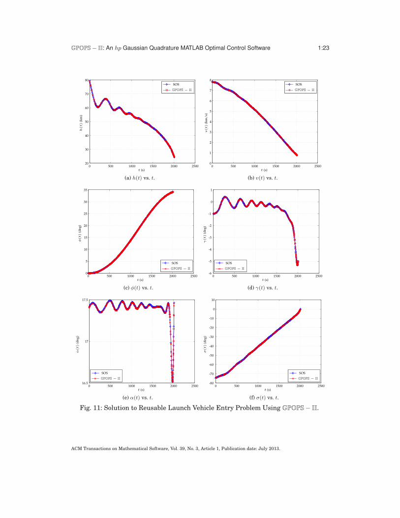
5.2. Reusable Launch Vehicle Entry
Consider the following optimal control problem of maximizing the crossrange duringthe atmospheric entry of a reusable launch vehicle and taken from Betts [2010] wherethe numerical values in Betts [2010] are converted from English units to SI units.Maximize the cost functional
J = φ(tf ) (60)
subject to the dynamic constraints
r = v sin γ , θ =v cos γ sinψ
r cosφ, φ =
v cos γ cosψ
r,
v = −D
m− g sin γ , γ =
L cosσ
mv−
(g
v−v
r
)
cos γ , ψ =L sinσ
mv cos γ+v cos γ sinψ tanφ
r,
(61)and the boundary conditions
h(0) = 79248 km , h(tf ) = 24384 km , θ(0) = 0 deg , θ(tf ) = Free,φ(0) = 0 deg , φ(tf ) = Free , v(0) = 7.803 km/s , v(tf ) = 0.762 km/sγ(0) = −1 deg , γ(tf ) = −5 deg , ψ(0) = 90 deg , ψ(tf ) = Free,
(62)where r = h + Re is the geocentric radius, h is the altitude, Re is the polar radius ofthe Earth, θ is the longitude, φ is the latitude, v is the speed, γ is the flight path angle,and ψ is the azimuth angle. Furthermore, the aerodynamic and gravitational forcesare computed as
D = ρv2SCD/2 , L = ρv2SCL/2 , g = µ/r2, (63)
where ρ = ρ0 exp(−h/H) is the atmospheric density, ρ0 is the density at sea level, H isthe density scale height, S is the vehicle reference area, CD is the coefficient of drag,CL is the coefficient of lift, and µ is the gravitational parameter.
The reusable launch vehicle entry optimal control problem was solved withGPOPS− II using the ph − (4, 10) mesh refinement method, an initial mesh consist-ing of ten evenly spaced mesh intervals with four LGR points per mesh interval, anda mesh refinement accuracy tolerance of 10−7, and the following initial guess:
h = linear(0, tf , h(0), h(tf )),θ = θ(0),φ = φ(0),v = linear(0, tf , v(0), v(tf )),γ = linear(0, tf , γ(0), γ(tf )),ψ = ψ(0),α = 0,σ = 0,tf = 1000 s.
The solution obtained using GPOPS− II is shown in Figs. 11a–11f alongside the so-lution obtained using the software Sparse Optimization Suite (SOS) [Betts 2010],where it is seen that the two solutions obtained are virtually indistinguishable. It isnoted that the optimal cost obtained by GPOPS− II and SOS are also nearly identi-cal at 0.59627639 and 0.59587608, respectively. Table II shows the performance of bothGPOPS− II and SOS on this example. It is interesting to see that GPOPS− II meetsthe accuracy tolerance of 10−7 in only four mesh iterations (three mesh refinements)while SOS requires a total of eight meshes (seven mesh refinements). Finally, the num-ber of collocation points used by GPOPS− II is approximately one half the number ofcollocation points required by SOS to achieve the same level of accuracy.
ACM Transactions on Mathematical Software, Vol. 39, No. 3, Article 1, Publication date: July 2013.
GPOPS− II: An hp Gaussian Quadrature MATLAB Optimal Control Software 1:23
SOS
GPOPS − II
t (s)
h(t)
(km
)
020
30
40
50
60
70
80
500 1500 25001000 2000
(a) h(t) vs. t.
SOS
GPOPS − II
t (s)
v(t)
(km
/s)
00
1
2
3
4
5
500 1500 2500
6
7
8
1000 2000
(b) v(t) vs. t.
SOS
GPOPS − II
t (s)
φ(t)
(deg
)
00
5
15
20
25
30
35
500 1500 2500
10
1000 2000
(c) φ(t) vs. t.
SOS
GPOPS − II
t (s)
γ(t)
(deg
)0
0
1
500 1500 2500-6
-5
-4
-3
-2
-1
1000 2000
(d) γ(t) vs. t.
SOS
GPOPS − II
t (s)
α(t)
(deg
)
16.5
17
17.5
0 500 1500 25001000 2000
(e) α(t) vs. t.
SOS
GPOPS − II
t (s)
σ(t)
(deg
)
-10
-20
-30
-40
-50
-60
-70
-80
0
0 500 1500 2500
10
1000 2000
(f) σ(t) vs. t.
Fig. 11: Solution to Reusable Launch Vehicle Entry Problem Using GPOPS− II.
ACM Transactions on Mathematical Software, Vol. 39, No. 3, Article 1, Publication date: July 2013.

1:24 M. A. Patterson and A. V. Rao
Table II: Performance of GPOPS− II on the Reusable Launch Vehicle Entry OptimalControl Problem.
Mesh Estimated Number of Estimated Number ofIteration Error (GPOPS− II) Collocation Points Error (SOS) Collocation Points
1 2.463× 10⁻³ 41 1.137× 10⁻² 512 2.946× 10⁻⁴ 103 1.326× 10⁻³ 1013 1.202× 10⁻⁵ 132 3.382× 10⁻⁵ 1014 8.704× 10⁻⁸ 175 1.314× 10⁻⁶ 1015 – – 2.364× 10⁻⁷ 2016 – – 2.364× 10⁻⁷ 2327 – – 1.006× 10⁻⁷ 3488 – – 9.933× 10⁻⁸ 353
5.3. Space Station Attitude Control
Consider the following space station attitude control optimal control problem takenfrom Pietz [2003] and Betts [2010]. Minimize the cost functional
J = 12
∫ tf
t0
uTudt (64)
subject to the dynamic constraints
ω = J−1 τ gg(r)− ω⊗ [Jω + h]− u ,
r = 12
[
rrT + I+ r]
[ω − ω(r)] ,
h = u,
(65)
the inequality path constraint‖h‖ ≤ hmax, (66)
and the boundary conditions
t0 = 0,tf = 1800,ω(0) = ω0,
r(0) = r0,
h(0) = h0,
0 = J−1 τ gg(r(tf ))− ω⊗(tf ) [Jω(tf ) + h(tf )] ,
0 = 12
[
r(tf )rT(tf ) + I+ r(tf )
]
[ω(tf )− ω0(r(tf ))] ,
(67)
where (ω, r,h) is the state and u is the control. In this formulation ω is the angularvelocity, r is the Euler-Rodrigues parameter vector, h is the angular momentum, andu is the input moment (and is the control).
ω0(r) = −ωorbC2,
τ gg = 3ω2orbC
⊗3 JC3,
(68)
and C2 and C3 are the second and third column, respectively, of the matrix
C = I+2
1 + rTr
(
r⊗r⊗ − r⊗)
. (69)
In this example the matrix J is given as
J =
2.80701911616× 10⁷ 4.822509936× 10⁵ −1.71675094448× 10⁷
4.822509936× 10⁵ 9.5144639344× 10⁷ 6.02604448× 10⁴
−1.71675094448× 10⁷ 6.02604448× 10⁴ 7.6594401336× 10⁷
, (70)
ACM Transactions on Mathematical Software, Vol. 39, No. 3, Article 1, Publication date: July 2013.

GPOPS− II: An hp Gaussian Quadrature MATLAB Optimal Control Software 1:25
while the initial conditions ω0, r0, and h0 are
ω0 =
−9.5380685844896× 10⁻⁶
−1.1363312657036× 10⁻³
+5.3472801108427× 10⁻⁶
,
r0 =
2.9963689649816× 10⁻³
1.5334477761054× 10⁻¹
3.8359805613992× 10⁻³
,
h0 =
[
500050005000
]
.
(71)
A more detailed description of this problem, including all of the constants J, ω0, r0,and h0, can be found in Pietz [2003] or Betts [2010].
The space station attitude control example was solved with GPOPS− II using theph − (4, 10) mesh refinement method with an initial mesh consisting of ten uniformlyspaced mesh intervals and four LGR points per mesh interval, a finite-difference per-turbation step size of 10−5, and the following initial guess:
ω = ω0
r = r0h = h0
u = 0,tf = 1800 s.
The state and control solutions obtained using GPOPS− II are shown, respectively,in Fig. 12 and 13 alongside the solution obtained using the optimal control softwareSparse Optimization Suite (SOS) [Betts 2013]. It is seen that the GPOPS− II solutionis in close agreement with the SOS solution. It is noted for this example that the meshrefinement accuracy tolerance of 10−6 was satisfied on the second mesh (that is, onemesh refinement iteration was performed) using a total of 46 collocation (LGR) points(that is, 47 total points when including the final time point).
ACM Transactions on Mathematical Software, Vol. 39, No. 3, Article 1, Publication date: July 2013.

1:26 M. A. Patterson and A. V. Rao
SOS
GPOPS − II
t (s)
ω1(t)×
10−
4
-8
-6
-4
-2
0
0
2
500 1500
6
4
1000 2000
(a) ω1(t) vs. t.
SOS
GPOPS − II
t (s)
ω2(t)×
10−
4
-11.6
-11.5
-11.4
-11.3
-11.2
-11.1
-11
-10.9
0 500 15001000 2000
(b) ω2(t) vs. t.
SOS
GPOPS − II
t (s)
ω3(t)×
10−
4
-3
-2
-1
0
0
1
2
3
5
500 1500
4
1000 2000
(c) ω3(t) vs. t.
SOS
GPOPS − II
t (s)
r1(t)
0
0 500 15001000 2000-0.05
0.05
0.1
0.15
(d) r1(t) vs. t.
SOS
GPOPS − II
t (s)
r2(t)
0 500 15000.144
0.146
0.148
0.152
0.154
0.156
0.158
1000 2000
0.15
(e) r2(t) vs. t.
SOS
GPOPS − II
t (s)r3(t)
00 500 15001000 2000
0.005
0.01
0.015
0.02
0.025
0.03
0.035
0.04
(f) r3(t) vs. t.
SOS
GPOPS − II
t (s)
h1(t)
-5
-10
0
0
5
500 1500
10
1000 2000
(g) h1(t) vs. t.
SOS
GPOPS − II
t (s)
h2(t)
-4
-2
0
0
2
500 1500
6
8
4
1000 2000
(h) h2(t) vs. t.
SOS
GPOPS − II
t (s)
h3(t)
-6
-4
-2
0
0
2
500 1500
6
4
1000 2000
(i) h3(t) vs. t.
Fig. 12: State Solution to Space Station Attitude Control Problem Using GPOPS− II
with the NLP Solver IPOPT and a Mesh Refinement Tolerance of 10−6 Alongside So-lution Obtained Using Optimal Control Software Sparse Optimization Suite.
ACM Transactions on Mathematical Software, Vol. 39, No. 3, Article 1, Publication date: July 2013.

GPOPS− II: An hp Gaussian Quadrature MATLAB Optimal Control Software 1:27
SOS
GPOPS − II
t (s)
u1(t)
-150
-100
-50
0
0
50
100
500 15001000 2000
(a) u1(t) vs. t.
SOS
GPOPS − II
t (s)
u2(t)
-5
-15
-10
0
0
5
15
20
25
500 1500
10
1000 2000
(b) u2(t) vs. t.
SOS
GPOPS − II
t (s)
u3(t) -10
-20
-30
-40
-50
0
0
20
500 1500
10
1000 2000
(c) u3(t) vs. t.
Fig. 13: Control Solution to Space Station Attitude Control Problem Using GPOPS− II
with the NLP Solver IPOPT and a Mesh Refinement Tolerance of 10−6 Alongside So-lution Obtained Using Optimal Control Software Sparse Optimization Suite.
5.4. Kinetic Batch Reactor
Consider the following three-phase kinetic batch reactor optimal control problem thatoriginally appears in the work of Leineweber [1998] and later appears in Betts [2010].Minimize the cost functional
J = γ1t(3)f + γ2p (72)
subject to the dynamic constraints
(73)
y(k)1 = −k2y
(k)2 u
(k)2 ,
y(k)2 = −k1y
(k)2 y
(k)6 + k−1u
(k)4 − k2y
(k)2 u
(k)4 ,
y(k)3 = k2y
(k)2 u
(k)2 + k3y
(k)4 y
(k)6 − k−3u
(k)3 ,
y(k)4 = −k3y
(k)4 y
(k)6 + k−3u
(k)3 ,
y(k)5 = k1y
(k)2 y
(k)6 − k−1u
(k)4 ,
y(k)6 = −k1y
(k)2 y
(k)6 + k−1u
(k)4 − k3y
(k)4 y
(k)6 + k−3u
(k)3 ,
, (k = 1, 2, 3), (74)
the equality path constraints
p− y(k)6 + 10−u
(k)1 − u
(k)2 − u
(k)3 − u
(k)4 = 0,
u(k)2 −K2y
(k)1 /(K2 + 10−u
(k)1 ) = 0,
u(k)3 −K3y
(k)3 /(K3 + 10−u
(k)1 ) = 0,
u(k)4 −K4y5/(K1 + 10−u
(k)1 ) = 0,
, (k = 1, 2, 3), (75)
the control inequality path constraint
293.15 ≤ u(k)5 ≤ 393.15, (k = 1, 2, 3), (76)
ACM Transactions on Mathematical Software, Vol. 39, No. 3, Article 1, Publication date: July 2013.

1:28 M. A. Patterson and A. V. Rao
the inequality path constraint in phases 1 and 2
y(k)4 ≤ a
[
t(k)]2
, (k = 1, 2), (77)
the interior point constraints
t(1)f = 0.01,
t(2)f = t
(3)f /4,
y(k)i = y
(k+1)i , (i = 1, . . . , 6, k = 1, 2, 3),
(78)
and the boundary conditions
y(1)1 (0) = 1.5776, y
(1)2 (0) = 8.32, y
(1)3 (0) = 0,
y(1)4 (0) = 0, y
(1)5 (0) = 0, y
(1)6 (0)− p = 0,
y(3)4 (t
(3)f ) ≤ 1,
(79)
where
k1 = k1 exp(−β1/u(k)5 ),
k−1 = k−1 exp(−β−1/u(k)5 ),
k2 = k2 exp(−β2/u(k)5 ),
k3 = k1,
k−3 = 12k−1,
, (k = 1, 2, 3), (80)
and the values for the parameters kj , βj , and Kj are given as
k1 = 1.3708× 10¹² , β1 = 9.2984× 10³ , K1 = 2.575× 10⁻¹⁶,
k−1 = 1.6215× 10²⁰ , β−1 = 1.3108× 10⁴ , K2 = 4.876× 10⁻¹⁴,
k2 = 5.2282× 10¹² , β2 = 9.599× 10³ , K3 = 1.7884× 10⁻¹⁶.
(81)
The kinetic batch reactor optimal control problem was solved using GPOPS− II us-ing the ph− (3, 6) mesh refinement method with an initial mesh in each phase consist-ing of ten uniformly spaced mesh intervals with three LGR points per mesh interval,a base derivative perturbation step size of 10−5, and the following linear initial guess
ACM Transactions on Mathematical Software, Vol. 39, No. 3, Article 1, Publication date: July 2013.

GPOPS− II: An hp Gaussian Quadrature MATLAB Optimal Control Software 1:29
(where the superscript represents the phase number):
y(1)1 = linear(t
(1)0 , t
(1)f , y1(0), 0.5),
y(1)2 = linear(t
(1)0 , t
(1)f , y2(0), 6),
y(1)3 = linear(t
(1)0 , t
(1)f , y3(0), 0.6),
y(1)4 = linear(t
(1)0 , t
(1)f , y4(0), 0.5),
y(1)5 = linear(t
(1)0 , t
(1)f , y5(0), 0.5),
y(1)6 = 0.013,
u(1)1 = linear(t
(1)0 , t
(1)f , 7, 10),
u(1)2 = 0,
u(1)3 = linear(t
(1)0 , t
(1)f , 0, 10−5),
u(1)4 = linear(t
(1)0 , t
(1)f , 0, 10−5),
u(1)5 = linear(t
(1)0 , t
(1)f , 373, 393.15).
t(1)0 = 0,
t(1)f = 0.01 hr,
y(2)1 = 0.5,
y(2)2 = 6,
y(2)3 = 0.6,
y(2)4 = 0.5,
y(2)5 = 0.5,
y(2)6 = 0.013,
u(2)1 = 10,
u(2)2 = 0,
u(2)3 = 10−5,
u(2)4 = 10−5,
u(2)5 = 393.15,
t(2)0 = 0.01 hr,t(2)f = 2.5 hr,
y(3)1 = linear(t
(3)0 , t
(3)f , 0.5, 0.1),
y(3)2 = linear(t
(3)0 , t
(3)f , 6, 5),
y(3)3 = 6,
y(3)4 = linear(t
(3)0 , t
(3)f , 0.5, 0.9),
y(3)5 = linear(t
(3)0 , t
(3)f , 0.5, 0.9),
y(3)6 = 0.013,
u(3)1 = 10,
u(3)2 = 0,
u(3)3 = 10−5,
u(3)4 = 10−5,
u(3)5 = 393.15,
t(3)0 = 2.5 hr,t(3)f = 10 hr.
The state and control solutions obtained using GPOPS− II are shown in Figs. 14–17, respectively, alongside the solution obtained using the software Sparse Optimiza-tion Suite (SOS) Betts [2013]. It is seen that in the complete three-phase problem theGPOPS− II and SOS solutions have the same trend, the key difference being that theGPOPS− II solution is shorter in duration than the SOS solution. A closer examina-tion, however, of the solution in phase 1 reveals that the two solutions are actuallyquite different at the start of the problem. The GPOPS− II solution moves away fromthe initial condition much more quickly than the SOS solution. Thus, the SOS solutionexhibits stiff behavior at the start of the solution while the GPOPS− II solution doesnot exhibit this stiffness. While the solutions are significantly different in phase 1, theoptimal cost obtained using GPOPS− II is 3.1650187 while the optimal cost obtained us-ing SOS is 3.1646696, leading to absolute and relative differences of only 3.4910× 10⁻⁴
and 1.1031 × 10⁻⁴, respectively. Thus, while the solutions obtained by each softwareprogram differ in the first (transient) phase, the overall performance of GPOPS− II issimilar to that obtained using SOS (particularly given the computational challenge ofthis example).
ACM Transactions on Mathematical Software, Vol. 39, No. 3, Article 1, Publication date: July 2013.

1:30 M. A. Patterson and A. V. Rao
SOS (Phase 1)
SOS (Phase 2)
SOS (Phase 3)
GPOPS − II (Phase 1)
GPOPS − II (Phase 2)
GPOPS − II (Phase 3)
t (hr)
y1(t)
00
1
1 2
0.2
0.4
0.5
0.6
1.2
1.4
1.5
1.6
1.8
(a) y1(t) vs. t.
SOS (Phase 1)
SOS (Phase 2)
SOS (Phase 3)
GPOPS − II (Phase 1)
GPOPS − II (Phase 2)
GPOPS − II (Phase 3)
t (hr)
y2(t)
0 1 2
6
7
8
0.5 1.55.5
6.5
7.5
8.5
(b) y2(t) vs. t.
0.3
SOS (Phase 1)
SOS (Phase 2)
SOS (Phase 3)
GPOPS − II (Phase 1)
GPOPS − II (Phase 2)
GPOPS − II (Phase 3)
t (hr)
y3(t)
00 1 2
0.2
0.4
0.5
0.5
0.6
0.7
1.5
0.1
(c) y3(t) vs. t.
SOS (Phase 1)
SOS (Phase 2)
SOS (Phase 3)
GPOPS − II (Phase 1)
GPOPS − II (Phase 2)
GPOPS − II (Phase 3)
t (hr)
y4(t)
0
0
1
1 2-0.2
0.2
0.4
0.5
0.6
1.2
1.5
1.8
(d) y4(t) vs. t.
SOS (Phase 1)
SOS (Phase 2)
SOS (Phase 3)
GPOPS − II (Phase 1)
GPOPS − II (Phase 2)
GPOPS − II (Phase 3)
t (hr)
y5(t)
00
1
1 2
0.2
0.4
0.5
0.6
1.2
1.4
1.5
1.8
(e) y5(t) vs. t.
SOS (Phase 1)
SOS (Phase 2)
SOS (Phase 3)
GPOPS − II (Phase 1)
GPOPS − II (Phase 2)
GPOPS − II (Phase 3)
t (hr)
y6(t)
00 1 20.5 1.5
0.005
0.01
0.015
(f) y6(t) vs. t.
Fig. 14: State Solution to Kinetic Batch Reactor Optimal Control Problem UsingGPOPS− II Alongside Solution Obtained Using Optimal Control Software Sparse Op-timization Suite.
ACM Transactions on Mathematical Software, Vol. 39, No. 3, Article 1, Publication date: July 2013.
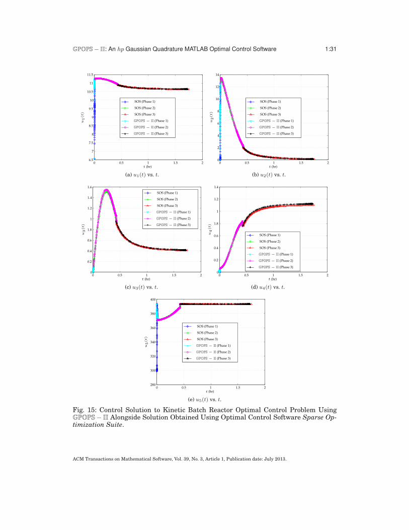
GPOPS− II: An hp Gaussian Quadrature MATLAB Optimal Control Software 1:31
SOS (Phase 1)
SOS (Phase 2)
SOS (Phase 3)
GPOPS − II (Phase 1)
GPOPS − II (Phase 2)
GPOPS − II (Phase 3)
t (hr)
u1(t)
0 1 2
7
8
9
10
11
0.5 1.56.5
7.5
8.5
9.5
10.5
11.5
(a) u1(t) vs. t.
SOS (Phase 1)
SOS (Phase 2)
SOS (Phase 3)
GPOPS − II (Phase 1)
GPOPS − II (Phase 2)
GPOPS − II (Phase 3)
t (hr)
u2(t)
00 1
2
2
4
6
8
10
12
0.5 1.5
14
(b) u2(t) vs. t.
SOS (Phase 1)
SOS (Phase 2)
SOS (Phase 3)
GPOPS − II (Phase 1)
GPOPS − II (Phase 2)
GPOPS − II (Phase 3)
t (hr)
u3(t)
00
1
1 2
0.2
0.4
0.5
0.6
1.2
1.4
1.5
1.6
1.8
(c) u3(t) vs. t.
SOS (Phase 1)
SOS (Phase 2)
SOS (Phase 3)
GPOPS − II (Phase 1)
GPOPS − II (Phase 2)
GPOPS − II (Phase 3)
t (hr)
u4(t)
00
1
1 2
0.2
0.4
0.5
0.6
1.2
1.4
1.5
1.8
(d) u4(t) vs. t.
SOS (Phase 1)
SOS (Phase 2)
SOS (Phase 3)
GPOPS − II (Phase 1)
GPOPS − II (Phase 2)
GPOPS − II (Phase 3)
t (hr)
u5(t)
0 1 20.5 1.5280
300
320
340
360
380
400
(e) u5(t) vs. t.
Fig. 15: Control Solution to Kinetic Batch Reactor Optimal Control Problem UsingGPOPS− II Alongside Solution Obtained Using Optimal Control Software Sparse Op-timization Suite.
ACM Transactions on Mathematical Software, Vol. 39, No. 3, Article 1, Publication date: July 2013.

1:32 M. A. Patterson and A. V. Rao
SOS (Phase 1)
GPOPS − II (Phase 1)
t (hr)
y1(t)
01.540
1.545
1.550
1.555
1.560
1.565
1.570
1.575
1.580
1.585
0.002 0.004 0.006 0.008 0.01
(a) y1(t) vs. t.
SOS (Phase 1)
GPOPS − II (Phase 1)
t (hr)
y2(t)
0 0.002 0.004 0.006 0.008 0.018.26
8.27
8.28
8.29
8.30
8.31
8.32
(b) y2(t) vs. t.
SOS (Phase 1)
GPOPS − II (Phase 1)
t (hr)
y3(t)
00 0.002 0.004
0.005
0.006 0.008
0.01
0.01
0.015
0.02
0.025
0.03
0.035
(c) y3(t) vs. t.
SOS (Phase 1)
GPOPS − II (Phase 1)
t (hr)
y4(t)×
10−
4
0
0
1
2
-0.5
0.5
1.5
2.5
0.002 0.004 0.006 0.008 0.01
(d) y4(t) vs. t.
0.012
0.014
SOS (Phase 1)
GPOPS − II (Phase 1)
t (hr)
y5(t)
00
0.002
0.002
0.004
0.004
0.006
0.006
0.008
0.008
0.01
0.01
(e) y5(t) vs. t.
SOS (Phase 1)
GPOPS − II (Phase 1)
t (hr)
y6(t)
00 0.002 0.004
0.005
0.006 0.008
0.01
0.01
0.015
(f) y6(t) vs. t.
Fig. 16: Phase 1 State Solution to Kinetic Batch Reactor Optimal Control Problem Us-ing GPOPS− II Alongside Solution Obtained Using Optimal Control Software SparseOptimization Suite.
ACM Transactions on Mathematical Software, Vol. 39, No. 3, Article 1, Publication date: July 2013.

GPOPS− II: An hp Gaussian Quadrature MATLAB Optimal Control Software 1:33
SOS (Phase 1)
GPOPS − II (Phase 1)
t (hr)
u1(t)
0
7
8
9
10
11
6.5
7.5
8.5
9.5
10.5
11.5
0.002 0.004 0.006 0.008 0.01
(a) u1(t) vs. t.
SOS (Phase 1)
GPOPS − II (Phase 1)
t (hr)
u2(t)
00
2
4
6
8
10
12
14
0.002 0.004 0.006 0.008 0.01
(b) u2(t) vs. t.
SOS (Phase 1)
GPOPS − II (Phase 1)
t (hr)
u3(t)
00 0.002 0.004 0.006 0.008
0.01
0.01
0.02
0.03
0.04
0.06
0.07
0.08
0.09
0.05
0.1
(c) u3(t) vs. t.
SOS (Phase 1)
GPOPS − II (Phase 1)
t (hr)
u4(t)
00 0.002 0.004 0.006 0.008
0.01
0.01
0.02
0.03
0.04
0.06
0.05
(d) u4(t) vs. t.
SOS (Phase 1)
GPOPS − II (Phase 1)
t (hr)
u5(t)
0280
300
320
340
360
380
400
0.002 0.004 0.006 0.008 0.01
(e) u5(t) vs. t.
Fig. 17: Phase 1 Control Solution to Kinetic Batch Reactor Optimal Control Prob-lem Using GPOPS− II Alongside Solution Obtained Using Optimal Control SoftwareSparse Optimization Suite.
ACM Transactions on Mathematical Software, Vol. 39, No. 3, Article 1, Publication date: July 2013.

1:34 M. A. Patterson and A. V. Rao
5.5. Multiple-Stage Launch Vehicle Ascent Problem
The problem considered in this section is the ascent of a multiple-stage launch vehicle.The objective is to maneuver the launch vehicle from the ground to the target orbitwhile maximizing the remaining fuel in the upper stage. It is noted that this exampleis is found verbatim in Benson [2004], Rao et al. [2010], and Betts [2010]. The problemis modeled using four phases where the objective is to maximize the mass at the endof the fourth phase, that is maximize
J = m(t(4)f ) (82)
subject to the dynamic constraints
r(p) = v(p),
v(p) = −
µ
‖r(p)‖3r(p) +
T (p)
m(p)u(p) +
D(p)
m(p),
m(p) = −T (p)
g0Isp,
(p = 1, . . . , 4), (83)
the initial conditionsr(t0) = r0 = (5605.2, 0, 3043.4)× 103 m,
v(t0) = v0 = (0, 0.4076, 0)× 103 m/s,m(t0) = m0 = 301454 kg.
(84)
the interior point constraints
r(p)(t(p)f )− r(p+1)(t
(p+10 ) = 0,
v(p)(t(p)f )− v(p+1)(t
(p+1)0 ) = 0, (p = 1, . . . , 3)
m(p)(t(p)f )−m
(p)dry −m(p+1)(t
(p+1)0 ) = 0,
(85)
the terminal constraints (corresponding to a geosynchronous transfer orbit),
a(t(4)f ) = af = 24361.14 km , e(t
(4)f ) = ef = 0.7308,
i(t(4)f ) = if = 28.5 deg , θ(t
(4)f ) = θf = 269.8 deg,
φ(t(4)f ) = φf = 130.5 deg,
(86)
and the path constraints
‖r(p)‖22 ≥ Re,‖u(p)‖22 = 1,
(p = 1, . . . , 4). (87)
In each phase r(t) = (x(t), y(t), z(t)) is the position relative to the center of the Earthexpressed in ECI coordinates, v = (vx(t), vy(t), vz(t)) is the inertial velocity expressedin ECI coordinates, µ is the gravitational parameter, T is the vacuum thrust, m is themass, g0 is the acceleration due to gravity at sea level, Isp is the specific impulse ofthe engine, u = (ux, uy, uz) is the thrust direction expressed in ECI coordinates, andD = (Dx, Dy, Dz) is the drag force expressed ECI coordinates. The drag force is definedas
D = − 12CDSρ‖vrel‖vrel (88)
where CD is the drag coefficient, S is the vehicle reference area, ρ = ρ0 exp(−h/H) isthe atmospheric density, ρ0 is the sea level density, h = r−Re is the altitude, r = ‖r‖2 =√
x2 + y2 + z2 is the geocentric radius,Re is the equatorial radius of the Earth,H is the
ACM Transactions on Mathematical Software, Vol. 39, No. 3, Article 1, Publication date: July 2013.

GPOPS− II: An hp Gaussian Quadrature MATLAB Optimal Control Software 1:35
density scale height, and vrel = v−ω× r is the velocity as viewed by an observer fixedto the Earth expressed in ECI coordinates, and ω = (0, 0,Ω) is the angular velocity ofthe Earth as viewed by an observer in the inertial reference frame expressed in ECIcoordinates. Furthermore, mdry is the dry mass of phases 1, 2, and 3 and is definedmdry = mtot − mprop, where mtot and mprop are, respectively, the total mass and drymass of phases 1, 2, and 3. Finally, the quantities a, e, i, θ, and φ are, respectively, thesemi-major axis, eccentricity, inclination, longitude of ascending node, and argument ofperiapsis, respectively. The vehicle data for this problem and the he numerical valuesfor the physical constants can be found in Tables III. and IV, respectively.
Table III: Vehicle Properties for Multiple-Stage Launch Vehicle Ascent Problem.
Quantity Solid Boosters Stage 1 Stage 2mtot (kg) 19290 104380 19300mprop (kg) 17010 95550 16820
T (N) 628500 1083100 110094Isp (s) 283.3 301.7 467.2
Number of Engines 9 1 1Burn Time (s) 75.2 261 700
Table IV: Constants Used in the Launch Vehicle Ascent Optimal Control Problem.
Constant ValuePayload Mass 4164 kg
S 4π m2
CD 0.5ρ0 1.225 kg/m3
H 7200 mt1 75.2 st2 150.4 st3 261 sRe 6378145 mΩ 7.29211585× 10⁻⁵ rad/sµ 3.986012× 10¹⁴ m3/s2
g0 9.80665 m/s2
The multiple-stage launch vehicle ascent optimal control problem was solved usingGPOPS− II with the NLP solver SNOPT and an initial mesh in each phase consistingof ten uniformly spaced mesh intervals with four LGR points per mesh interval, and
ACM Transactions on Mathematical Software, Vol. 39, No. 3, Article 1, Publication date: July 2013.

1:36 M. A. Patterson and A. V. Rao
the following initial guess:
r(1) = r(0),v(1) = v(0),
m(1) = linear(t(1)0 , t
(1)f , 3.01454, 1.71863)× 105 kg,
u(1) = (0, 1, 0),
t(1)0 = 0,
t(1)f = 75.2 s,
r(2) = r(0),v(2) = v(0),
m(2) = linear(t(2)0 , t
(2)f , 1.58184, 0.796238)× 105 kg,
u(2) = (0, 1, 0),
t(2)0 = 75.2 s,t(2)f = 150.4 s,
r(3) = r,v(3) = v,
m(3) = linear(t(3)0 , t
(3)f , 7.27838, 3.22940)× 104 kg,
u(3) = (0, 1, 0),
t(3)0 = 150.4 s,t(3)f = 261 s,
r(4) = r,v(4) = v,
m(4) = linear(t(4)0 , t
(4)f , 2.34640, 0.41640)× 104 kg,
u(4) = (0, 1, 0),
t(4)0 = 261 s,t(4)f = 961 s,
where (r, v) are obtained from a conversion of the orbital elements (a, e, i, θ, φ, ν) =(af , ef , if , θf , φf , 0) to ECI Cartesian coordinates [Bate et al. 1971] and ν is the trueanomaly. The GPOPS− II solution is shown in Fig. 18. In this example the mesh re-finement accuracy tolerance of 10−6 is satisfied on the initial mesh and, thus, no meshrefinement is performed. The solution obtained using GPOPS− II matches closely withthe solution obtained using the software SOCS [Betts 2010], where it is noted that theoptimal objective values obtained using GPOPS− II and SOCS are −7529.712680 and−7529.712412, respectively.
ACM Transactions on Mathematical Software, Vol. 39, No. 3, Article 1, Publication date: July 2013.

GPOPS− II: An hp Gaussian Quadrature MATLAB Optimal Control Software 1:37
Phase 1
Phase 2
Phase 3
Phase 4
t (s)
h(t)
(km
)
50
100
150
00
200
200
250
400 600 800 1000
(a) h(t) vs. t.
Phase 1
Phase 2
Phase 3
Phase 4
t (s)
v(t)
(m/
s)
00 200 400 600 800 1000
2000
4000
6000
8000
10000
12000
(b) v(t) vs. t.
Phase 1
Phase 2
Phase 3
Phase 4
t (s)
m(t)×
1000
(kg
)
50
100
150
00
200
200
250
300
350
400 600 800 1000
(c) m(t) vs. t.
Phase 1
Phase 2
Phase 3
Phase 4
t (s)
u1(t)
-0.8
-0.6
-0.4
-0.2
0.2
0.4
0.6
0.8
0
0
1
200 400 600 800 1000
(d) u1(t) vs. t.
Phase 1
Phase 2
Phase 3
Phase 4
t (s)
u2(t)
0.4
0.5
0.6
0.7
0.8
0.9
0
1
200 400 600 800 1000
(e) u2(t) vs. t.
Phase 1
Phase 2
Phase 3
Phase 4
t (s)
u3(t)
-0.4
-0.3
-0.2
-0.1
0.1
0.2
0.3
0.4
0.5
0
0 200 400 600 800 1000
(f) u3(t) vs. t.
Fig. 18: Solution of Multiple-Stage Launch Vehicle Ascent Problem Using GPOPS− II.
ACM Transactions on Mathematical Software, Vol. 39, No. 3, Article 1, Publication date: July 2013.

1:38 M. A. Patterson and A. V. Rao
6. CAPABILITIES OF GPOPS− II
The five examples provide in Section 5 highlight the capability of GPOPS− II to solvea wide variety of problems. First, the hyper-sensitive example shows the capability ofthe ph mesh refinement method in increasing the number of mesh intervals and col-location points in regions where the dynamics are changing more rapidly, while thereusable launch vehicle entry example demonstrates the ability of the ph mesh refine-ment method to keep the number of collocation points much smaller than might be pos-sible using a fixed low-order collocation method. Second, the space station attitude con-trol and kinetic batch reactor examples demonstrate the flexibility of the software toachieve better performance on an application by modifying the default settings. Third,the launch vehicle ascent problem shows that GPOPS− II has been designed with theability to employ different NLP solvers. The different examples also demonstrate thewide variety of problems that can be formulated in GPOPS− II. Such problems rangefrom one-phase problems with a Lagrange cost (for example, the hyper-sensitive andspace station attitude control examples), Mayer cost (for example, the reusable launchvehicle entry and launch vehicle ascent examples), and problems that include staticparameters (for example, the kinetic batch reactor example). Moreover, it was shownthat GPOPS− II has the ability to solve challenging multiple-phase problems (for ex-ample, the kinetic batch reactor example). The fact that GPOPS− II is capable of solv-ing the challenging benchmark optimal control problems shown in this paper showsthe general utility of the software on problems that may arise in different applicationareas.
7. LIMITATIONS OF GPOPS− II
Like all software, GPOPS− II has limitations. First, it is assumed in the implementa-tion that all functions have continuous first and second derivatives. In some applica-tions, however, the functions themselves may be continuous while the derivatives maybe discontinuous. In such problems GPOPS− II may struggle because the NLP solveris not being provided with accurate approximations to the derivative functions. Fur-thermore, the ability of any given NLP solver to obtain a solution is always problemdependent. As a result, for some examples it may be the case that IPOPT will per-form better than SNOPT, but in some cases SNOPT may may significantly outperformIPOPT (the launch vehicle ascent problem is an example where SNOPT outperformsIPOPT with GPOPS− II). Also, problems with high-index path constraints may resultin the constraint qualification conditions not being satisfied on fine meshes. In suchcases, unique NLP Lagrange multipliers may not exist. In some cases, these Lagrangemultipliers may become unbounded. Finally, as is true for many optimal control soft-ware programs, applications whose solutions lie on a singular arc can create problemsdue to the inability to determine the optimal control along the singular arc. In suchcases highly inaccurate solution may be obtained in the region near the singular arc,and mesh refinement may only exacerbate these inaccuracies. The approach for prob-lems whose solutions lie on a singular arc is to modify the problem by including theconditions that define the singular arc (thus removing the singularity).
8. CONCLUSIONS
A general-purpose MATLAB software program called GPOPS− II has been describedfor solving multiple-phase optimal control problems using variable-order Gaussianquadrature methods. In particular, the software employs a Legendre-Gauss-Radauquadrature orthogonal collocation where the continuous-time control problem is tran-scribed to a large sparse nonlinear programming problem. The software implementstwo previously developed adaptive mesh refinement methods that allow for flexibility
ACM Transactions on Mathematical Software, Vol. 39, No. 3, Article 1, Publication date: July 2013.

GPOPS− II: An hp Gaussian Quadrature MATLAB Optimal Control Software 1:39
in the number and placement of the collocation and mesh points in order to achievea specified accuracy. In addition, the software is designed to compute all derivativesrequired by the NLP solver using sparse finite-differencing of the optimal control func-tions. The key components of the software have been described in detail and the utilityof the software is demonstrated on five benchmark optimal control problems. The soft-ware described in this paper provides researchers a useful platform upon which tosolve a wide variety of complex constrained optimal control problems.
Acknowledgments
The authors gratefully acknowledge support for this research from the U.S. Office ofNaval Research under Grant N00014-11-1-0068 and from the U.S. Defense AdvancedResearch Projects Agency under Contract HR0011-12-C-0011.
Disclaimer
The views expressed are those of the authors and do not reflect the official policy orposition of the Department of Defense or the U.S. Government.
REFERENCES
ABRAMOWITZ, M. AND STEGUN, I. 1965. Handbook of Mathematical Functions with Formulas, Graphs, andMathematical Tables. Dover Publications, New York.
BABUSKA, I. AND RHEINBOLDT, W. C. 1979. Reliable error estimation and mesh adaptation for the finiteelement method. In Proc. Second Intl. Conf. Computational Methods in Nonlinear Mechanics (Univ.Texas Austin). North-Holland, Amsterdam-New York, 67–108.
BABUSKA, I. AND RHEINBOLDT, W. C. 1981. A posteriori error analysis of finite element solutions for one-dimensional problems. SIAM Journal on Numerical Analysis 18, 565–589.
BABUSKA, I. AND RHEINBOLDT, W. C. 1982. Computational error estimates and adaptive processes forsome nonlinear structural problems. Computer Methods in Applied Mechanics and Engineering 34, 1–3,895–937.
BABUSKA, I., ZIENKIEWICZ, O. C., GAGO, J., AND DE A. OLIVEIRA, E. R. 1986. Accuracy Estimates andAdaptive Refinements in Finite Element Computations. John Wiley & Sons, Chichester.
BATE, R. R., MUELLER, D. D., AND WHITE, J. E. 1971. Fundamentals of Astrodynamics. Dover Publica-tions, Mineola, New York.
BECERRA, V. M. 2009. PSOPT Optimal Control Solver User Manual. University of Reading.http://www.psopt.org.
BENSON, D. A. 2004. A Gauss pseudospectral transcription for optimal control. Ph.D. thesis, Department ofAeronautics and Astronautics, Massachusetts Institute of Technology, Cambridge, Massachusetts.
BENSON, D. A., HUNTINGTON, G. T., THORVALDSEN, T. P., AND RAO, A. V. 2006. Direct trajectory opti-mization and costate estimation via an orthogonal collocation method. Journal of Guidance, Control,and Dynamics 29, 6, 1435–1440.
BETTS, J. T. 1990. Sparse jacobian updates in the collocation method for optimal control problems. Journalof Guidance, Control, and Dynamics 13, 3, 409–415.
BETTS, J. T. 1998. Survey of numerical methods for trajectory optimization. Journal of Guidnance, Control,and Dynamics 21, 2, 193–207.
BETTS, J. T. 2010. Practical Methods for Optimal Control and Estimation Using Nonlinear Programming.SIAM Press, Philadelphia.
BETTS, J. T. 2013. Sparse Optimization Suite (SOS). Applied Mathematical Analysis, LLC, Based on theAlgorithms Published in Betts, J. T., Practical Methods for Optimal Control and Estimation Using Non-linear Programming, SIAM Press, Philadelphia, 2010.
BIEGLER, L. T., GHATTAS, O., HEINKENSCHLOSS, M., AND VAN BLOEMEN WAANDERS, B., Eds. 2003.Large-Scale PDE Constrained Optimization. Lecture Notes in Computational Science and Engineering,Vol. 30. Springer-Verlag, Berlin.
BIEGLER, L. T. AND ZAVALA, V. M. 2008. Large-scale nonlinear programming using IPOPT: An integratingframework for enterprise-wide optimization. Computers and Chemical Engineering 33, 3, 575–582.
BYRD, R. H., NOCEDAL, J., AND WALTZ, R. A. 2006. Knitro: An integrated package for nonlinear optimiza-tion. In Large Scale Nonlinear Optimization. Springer Verlag, 35–59.
ACM Transactions on Mathematical Software, Vol. 39, No. 3, Article 1, Publication date: July 2013.

1:40 M. A. Patterson and A. V. Rao
CANUTO, C., HUSSAINI, M. Y., QUARTERONI, A., AND ZANG, T. A. 1988. Spectral Methods in Fluid Dy-namics. Spinger-Verlag, Heidelberg, Germany.
DARBY, C. L., GARG, D., AND RAO, A. V. 2011a. Costate estimation using multiple-interval pseudospectralmethods. Journal of Spacecraft and Rockets 48, 5, 856–866.
DARBY, C. L., HAGER, W. W., AND RAO, A. V. 2011b. Direct trajectory optimization using a variable low-order adaptive pseudospectral method. Journal of Spacecraft and Rockets 48, 3, 433–445.
DARBY, C. L., HAGER, W. W., AND RAO, A. V. 2011c. An hp-adaptive pseudospectral method for solvingoptimal control problems. Optimal Control Applications and Methods 32, 4, 476–502.
ELNAGAR, G., KAZEMI, M., AND RAZZAGHI, M. 1995. The pseudospectral Legendre method for discretizingoptimal control problems. IEEE Transactions on Automatic Control 40, 10, 1793–1796.
ELNAGAR, G. AND RAZZAGHI, M. 1998. A collocation-type method for linear quadratic optimal control prob-lems. Optimal Control Applications and Methods 18, 3, 227–235.
FALUGI, P., KERRIGAN, E., AND VAN WYK, E. 2010. Imperial College London Optimal Control SoftwareUser Guide (ICLOCS). Department of Electrical Engineering, Imperial College London, London, UK.
FORNBERG, B. 1998. A Practical Guide to Pseudospectral Methods. Cambridge University Press, New York.GARG, D., HAGER, W. W., AND RAO, A. V. 2011a. Pseudospectral methods for solving infinite-horizon opti-
mal control problems. Automatica 47, 4, 829–837.GARG, D., PATTERSON, M., FRANCOLIN, C., DARBY, C., HUNTINGTON, G., HAGER, W. W., AND RAO, A. V.
2011b. Direct trajectory optimization and costate estimation of finite-horizon and infinite-horizon opti-mal control problems using a Radau pseudospectral method. Computational Optimization and Applica-tions 49, 2, 335–358.
GARG, D., PATTERSON, M., HAGER, W. W., RAO, A. V., BENSON, D. A., AND HUNTINGTON, G. T. 2010. Aunified framework for the numerical solution of optimal control problems using pseudospectral methods.Automatica 46, 11, 1843–1851.
GILL, P. E., MURRAY, W., AND SAUNDERS, M. A. 2002. SNOPT: An SQP algorithm for large-scale con-strained optimization. SIAM Review 47, 1, 99–131.
GILL, P. E., MURRAY, W., AND WRIGHT, M. H. 1981. Practical Optimization. Academic Press, London.GOH, C. J. AND TEO, K. L. 1988. Control parameterization: A unified approach to optimal control problems
with general constraints. Automatica 24, 1, 3–18.GONG, Q., FAHROO, F., AND ROSS, I. M. 2008a. Spectral algorithm for pseudospectral methods in optimal
control. Journal of Guidance, Control and Dynamics 31, 3, 460–471.GONG, Q., ROSS, I. M., KANG, W., AND FAHROO, F. 2008b. Connections between the covector mapping the-
orem and convergence of pseudospectral methods. Computational Optimization and Applications 41, 3,307–335.
HOUSKA, B., FERREAU, H. J., AND DIEHL, M. 2011. ACADO toolkit – an open-source framework for auto-matic control and dynamic optimization. Optimal Control Applications and Methods 32, 3, 298–312.
HUNTINGTON, G. T., BENSON, D. A., AND RAO, A. V. 2007. Optimal configuration of tetrahedral spacecraftformations. The Journal of the Astronautical Sciences 55, 2, 141–169.
HUNTINGTON, G. T. AND RAO, A. V. 2008. Optimal reconfiguration of spacecraft formations using the Gausspseudospectral method. Journal of Guidance, Control, and Dynamics 31, 3, 689–698.
JAIN, D. AND TSIOTRAS, P. 2008. Trajectory optimization using multiresolution techniques. Journal ofGuidance, Control, and Dynamics 31, 5, 1424–1436.
JANSCH, C., WELL, K. H., AND SCHNEPPER, K. 1994. GESOP - Eine Software Umgebung Zur SimulationUnd Optimierung. Proceedings des SFB.
KAMESWARAN, S. AND BIEGLER, L. T. 2008. Convergence rates for direct transcription of optimal controlproblems using collocation at Radau points. Computational Optimization and Applications 41, 1, 81–126.
LEINEWEBER, D. B. 1998. Efficient reduced SQP methods for the optimization of chemical processes de-scribed by large space dae models. Ph.D. thesis, Universität Heidelberg, Interdisziplinäres Zentrum fürWissenschaftliches Rechnen (IWR).
MUMPS. 2011. Multifrontal massively parallel solver (mumps 4.10.0) user’s guide.PATTERSON, M. A. AND RAO, A. V. 2012. Exploiting sparsity in direct collocation pseudospectral methods
for solving optimal control problems. Journal of Spacecraft and Rockets 49, 2, 364–377.PATTERSON, M. A., RAO, A. V., AND HAGER, W. W. 2013. A ph collocation scheme for optimal control.
Optimal Control Applications and Methods, In Revision.PIETZ, J. A. 2003. Pseudospectral collocation methods for the direct transcription of optimal control prob-
lems. M.S. thesis, Rice University, Houston, Texas.
ACM Transactions on Mathematical Software, Vol. 39, No. 3, Article 1, Publication date: July 2013.

GPOPS− II: An hp Gaussian Quadrature MATLAB Optimal Control Software 1:41
ÅKESSON, J., ARZEN, K. E., GÄFERT, M., BERGDAHL, T., AND TUMMESCHEIT, H. 2010. Modeling andOptimization with Optimica and JModelica.org – Languages and Tools for Solving Large-Scale DynamicOptimization Problems. Computers and Chemical Engineering 34, 11, 1737–1749.
RAO, A. V., BENSON, D. A., DARBY, C., PATTERSON, M. A., FRANCOLIN, C., SANDERS, I., AND HUNT-INGTON, G. T. 2010. Algorithm 902: GPOPS, A MATLAB software for solving multiple-phase optimalcontrol problems using the Gauss pseudospectral method. ACM Transactions on Mathematical Soft-ware 37, 2, 22:1–22:39.
RAO, A. V. AND MEASE, K. D. 2000. Eigenvector approximate dichotomic basis method for solving hyper-sensitive optimal control problems. Optimal Control Applications and Methods 21, 1, 1–19.
TREFETHEN, L. N. 2000. Spectral Methods Using MATLAB. SIAM Press, Philadelphia.VLASES, W. G., PARIS, S. W., LAJOIE, R. M., MARTENS, M. J., AND HARGRAVES, C. R. 1990. Optimal
trajectories by implicit simulation. Tech. Rep. WRDC-TR-90-3056, Boeing Aerospace and Electronics,Wright-Patterson Air Force Base, Ohio.
VON STRYK, O. 2000. User’s Guide for DIRCOL (Version 2.1): A Direct Collocation Method for the NumericalSolution of Optimal Control Problems. Technical University, Munich, Germany.
WÄCHTER, A. AND BIEGLER, L. T. 2006. On the implementation of an interior-point filter line-search algo-rithm for large-scale nonlinear programming. Mathematical Programming 106, 1, 25–57.
ZHAO, Y. AND TSIOTRAS, P. 2011. Density functions for mesh refinement in numerical optimal control.Journal of Guidance, Control, and Dynamics 34, 1, 271–277.
ACM Transactions on Mathematical Software, Vol. 39, No. 3, Article 1, Publication date: July 2013.