1, A brief review about Quantum Mechanics 1. Basic Quantum...

1, A brief review about Quantum Mechanics

1. Basic Quantum Theory

2. Time-Dependent Perturbation Theory

3. Simple Harmonic Oscillator

4. Quantization of the field

5. Canonical Quantization

Ref:

Ch. 2 in ”Introductory Quantum Optics,” by C. Gerry and P. Knight.Ch. 2 in ”Mesoscopic Quantum Optics,” by Y. Yamamoto and A. Imamoglu.Ch. 1 in ”Quantum Optics,” by D. Wall and G. Milburn.Ch. 4 in ”The Quantum Theory of Light,” by R. Loudon.Ch. 1, 2, 3, 6 in ”Mathematical Methods of Quantum Optics,” by R. PuriCh. 3 in ”Elements of Quantum Optics,” by P. Meystre and M. Sargent III.Ch. 9 in ”Modern Foundations of Quantum Optics,” by V. Vedral.

IPT5340, Spring ’08 – p. 1/51

Field Quantization

1. Simple Harmonic Oscillator

2. Quantization of a single-mode field

3. Basic Quantum Theory

4. Time-Dependent Perturbation Theory

5. Canonical Quantization

6. Quantum fluctuations of a single-mode field

7. Quadrature operators for a single-mode field

8. Multimode fields

9. Thermal fields

10. Vacuum fluctuations and the zero-point energy

11. Casimir force

IPT5340, Spring ’08 – p. 2/51

Role of Quantum Optics

photons occupy an electromagnetic mode,we will always refer to modes in quantum optics,typically a plane wave;

the energy in a mode is not continuous but discrete inquanta of ~ω;

the observables are just represented by probabilitiesas usual in quantum mechanics;

there is a zero point energy inherent to each mode whichis equivalent with fluctuations of the electromagneticfield in vacuum, due to uncertainty principle.

quantized fields and quantum fluctuations (zero-point energy)

IPT5340, Spring ’08 – p. 3/51

Vacuum

vacuum is not just nothing, it is full of energy.

IPT5340, Spring ’08 – p. 4/51

Vacuum

spontaneous emission is actually stimulated by the vacuum fluctuation of theelectromagnetic field,

one can modify vacuum fluctuations by resonators and photonic crystals,

atomic stability : the electron does not crash into the core due to vacuum fluctuationof the electromagnetic field,

gravity is not a fundamental force but a side effect matter modifies the vacuumfluctuations, by Sakharov,

Casimir effect : two charged metal plates repel each other until Casimir effectovercomes the repulsion,

Lamb shift : the energy level difference between 2S1/2 and 2P1/2 in hydrogen.

. . .

IPT5340, Spring ’08 – p. 5/51

Simple Harmonic Oscillator

The simple harmonic oscillator has no driving force, and no friction (damping), sothe net force is just:

F = −kx = ma = md2x

dt2,

if define ω20 = k/m, then

d2x

dt2+ ω0

2x = 0

the general solution x = ACos(ω0t+ φ) ,

The kinetic energy is T = 12m

“

dxdt

”2= 1

2kA2 sin2(ω0t+ φ),

the potential energy is U = 12kx2 = 1

2kA2 cos2(ω0t+ φ)

the total energy of the system has the constant value E = 12kA2.

IPT5340, Spring ’08 – p. 6/51

Quantum Harmonic Oscillator: 1D

In the one-dimensional harmonic oscillator problem, a particle of mass m is

subject to a potential V (x) =1

2mω2x2.

In classical mechanics, mω2 = k is called the spring stiffness coefficient or forceconstant, and ω the circular frequency.

The Hamiltonian of the particle is: H = p2

2m+ 1

2mω2x2 where x is the position

operator, and p is the momentum operator“

p = −i~ ddx

”

. The first term

represents the kinetic energy of the particle, and the second term represents thepotential energy in which it resides.

IPT5340, Spring ’08 – p. 7/51

Maxwell’s equations in Free space

Faraday’s law:

∇× E = −∂

∂ tB,

Ampére’s law:

∇× H =∂

∂ tD,

Gauss’s law for the electric field:

∇ · D = 0,

Gauss’s law for the magnetic field:

∇ · B = 0,

the constitutive relation: B = µ0H and D = ǫ0E.IPT5340, Spring ’08 – p. 8/51

Plane electromagnetic waves

Maxwell’s equations in free space, there is vacuum, no free charges, no currents,J = ρ = 0,

both E and B satisfy wave equation,∇2E = ǫ0µ0∂2E∂t2

,

we can use the solutions of wave optics,

E(r, t) = E0exp(iωt)exp(−ik · r),B(r, t) = B0exp(iωt)exp(−ik · r),

IPT5340, Spring ’08 – p. 9/51

Mode Expansion of the Field

A single-mode field, polarized along the x-direction, in the cavity:

E(r, t) = xEx(z, t) =X

j

(2mjω

2j

V ǫ0)1/2qj(t)Sin(kjz),

where k = ω/c, ωj = c(jπ/L), j = 1, 2, . . . , V is the effective volume of thecavity, and q(t) is the normal mode amplitude with the dimension of a length (actsas a canonical position, and pj = mj qj is the canonical momentum).

the magnetic field in the cavity:

H(r, t) = yHy(z, t) = (mj2ω2

j

V ǫ0)1/2(

qj(t)ǫ0kj

)Cos(kjz),

the classical Hamiltonian for the field:

H =1

2

Z

VdV [ǫ0E

2x + µ0H

2y ],

=1

2

X

j

[mjω2mq

2j +mj q

2j ] =

1

2

X

j

[mjω2mq

2j +

p2j

mj].

IPT5340, Spring ’08 – p. 10/51

Quantization of the Electromagnetic Field

Like simple harmonic oscillator, H = p2

2m+ 1

2kx2, where [x, p] = i~,

For EM field, H = 12

P

j [mjω2mq

2j +

p2

j

mj], where [qi, pj ] = i~δij ,

annihilation and creation operators:

aje−iωjt =

1p

2mj~ωj

(mjωj qj + ipj),

a†jeiωjt =

1p

2mj~ωj

(mjωj qj − ipj),

the Hamiltonian for EM fields becomes: H =P

j ~ωj(a†j aj + 1

2),

the electric and magnetic fields become,

Ex(z, t) =X

j

(~ωj

ǫ0V)1/2[aje

−iωjt + a†jeiωjt]Sin(kjz),

Hy(z, t) = −iǫ0cX

j

(~ωj

ǫ0V)1/2[aje

−iωjt − a†jeiωjt]Cos(kjz),

IPT5340, Spring ’08 – p. 11/51

Quantization of EM fields

the Hamiltonian for EM fields becomes: H =P

j ~ωj(a†j aj + 1

2),


Ex(z, t) =X

j

(~ωj

ǫ0V)1/2[aje

−iωjt + a†jeiωjt] sin(kjz),

=X

j

cj [a1j cosωjt+ a2j sinωjt]uj(r),

IPT5340, Spring ’08 – p. 12/51

Simple Harmonic Oscillator in Schrödinger picture

one-dimensional harmonic oscillator, H = p2

2m+ 1

2kx2,

Schrödinger equation,

d2

dx2ψ(x) +

2m

~2[E − 1

2kx2]ψ(x) = 0,

with dimensionless coordinates ξ =p

mω/~x and dimensionless quantityǫ = 2E/~ω, we have

d2

dξ2ψ(x) + [ǫ− ξ2]ψ(x) = 0,

which has Hermite-Gaussian solutions,

ψ(ξ) = Hn(ξ)e−ξ2/2, E =1

2~ωǫ = ~ω(n+

1

2),

where n = 0, 1, 2, . . .

Ch. 7 in ”Quantum Mechanics,” by A. Goswami.Ch. 2 in ”Modern Quantum Mechanics,” by J. Sakurai.

IPT5340, Spring ’08 – p. 13/51

Quantum Harmonic Oscillator

d2

dξ2ψ(x) + [ǫ− ξ2]ψ(x) = 0,

which has Hermite-Gaussian solutions,

ψ(ξ) = Hn(ξ)e−ξ2/2, E =1

2~ωǫ = ~ω(n+

1

2),

where n = 0, 1, 2, . . .

IPT5340, Spring ’08 – p. 14/51

Simple Harmonic Oscillator: operator method

one-dimensional harmonic oscillator, H = p2

2m+ 1

2kx2, where [x, p] = i~

define annihilation operator (destruction, lowering, or step-down operators):

a =p

mω/2~x+ ip/√

2m~ω.

define creation operator (raising, or step-up operators):

a† =p

mω/2~x− ip/√

2m~ω.

note that a and a† are not hermitian operators, but (a†)† = a.

the commutation relation for a and a† is [a, a†] = 1.

the oscillator Hamiltonian can be written as,

H = ~ω(a†a+1

2) = ~ω(N +

1

2),

where N is called the number operator, which is hermitian.

IPT5340, Spring ’08 – p. 15/51


normalization of the eigenstates, (a†)n|Ψ0〉 = cn|Ψn〉, where cn =√n.

a|Ψn〉 =√n|Ψn−1〉,

a†|Ψn〉 =√n+ 1|Ψn+1〉,

x-representation, Ψn(x) = 〈x|Ψn〉.

ground state, 〈x|a|Ψ0〉 = 0, i.e.

[

r

mω

2~x+ ~

1√2m~ω

d

dx]Ψ0(x) = 0,

define a dimensionless variable ξ =p

mω/~x, we obtain

(ξ +ddξ

)Ψ0 = 0,

with the solution Ψ0(ξ) = c0exp(−ξ2/2).

IPT5340, Spring ’08 – p. 17/51

brain-storms

Damped harmonic oscillator: d2xdt2

+ bm

dxdt

+ ω02x = 0,

where b is an experimentally determined damping constant satisfying therelationship F = −bv. An example of a system obeying this equation would be aweighted spring underwater if the damping force exerted by the water is assumedto be linearly proportional to v.

Mode expansion of the field in other bases, e.x. spherical wave:

E(r) =A

|r − r0|exp(−ik|r − r0|),

How to quantize fields?

IPT5340, Spring ’08 – p. 18/51

Postulates of Quantum Mechanics

Postulate 1 : An isolated quantum system is described by a vector in a Hilbert space. Twovectors differing only by a multiplying constant represent the same physical state.

quantum state: |Ψ〉 =P

i αi|ψi〉,

completeness:P

i |ψi〉〈ψi| = I ,

probability interpretation (projection): Ψ(x) = 〈x|Ψ〉,

operator: A|Ψ〉 = |Φ〉,

representation: 〈φ|A|ψ〉,

adjoint of A: 〈φ|A|ψ〉 = 〈ψ|A†|φ〉∗,

hermitian operator: H = H†,

unitary operator: U U† = U†U = I .

Ch. 1-5 in ”The Principles of Quantum Mechanics,” by P. Dirac.Ch. 1 in ”Mathematical Methods of Quantum Optics,” by R. Puri.

IPT5340, Spring ’08 – p. 19/51

Operators

For a unitary operator, 〈ψi|ψj〉 = 〈ψi|U†Uψj〉, the set of states U |ψ〉 preservesthe scalar product.

U can be represented as U = exp(iH) if H is hermitian.

normal operator: [A, A†] = 0, the eigenstates of only a normal operator areorthonormal.i.e. hermitian and unitary operators are normal operators.

The sum of the diagonal elements 〈φ|A|ψ〉 is call the trace of A,

Tr(A) =X

i

〈φi|A|φi〉,

The value of the trace of an operator is independent of the basis.

The eigenvalues of a hermitian operator are real, H|Ψ〉 = λ|Ψ〉, where λ is real.

If A and B do not commute then they do not admit a common set of eigenvectors.

IPT5340, Spring ’08 – p. 20/51

Postulates of Quantum Mechanics

Postulate 2 : To each dynamical variable there corresponds a unique hermitian operator.Postulate 3 : If A and B are hermitian operators corresponding to classical dynamicalvariables a and b, then the commutator of A and B is given by

[A, B] ≡ AB − BA = i~{a, b},

where {a, b} is the classical Poisson bracket.Postulate 4 : Each act of measurement of an observable A of a system in state |Ψ〉collapses the system to an eigenstate |ψi〉 of A with probability |〈φi|Ψ〉|2.The average or the expectation value of A is given by

〈A〉 =X

i

λi|〈φi|Ψ〉|2 = 〈Ψ|A|Ψ〉,

where λi is the eigenvalue of A corresponding to the eigenstate |ψi〉.

IPT5340, Spring ’08 – p. 21/51

Uncertainty relation

Non-commuting observable do not admit common eigenvectors.

Non-commuting observables can not have definite values simultaneously.

Simultaneous measurement of non-commuting observables to an arbitrary degreeof accuracy is thus incompatible.

variance: ∆A2 = 〈Ψ|(A− 〈A〉)2|Ψ〉 = 〈Ψ|A2|Ψ〉 − 〈Ψ|A|Ψ〉2.

∆A2∆B2 ≥ 1

4[〈F 〉2 + 〈C〉2],

where

[A, B] = iC, and F = AB + BA− 2〈A〉〈B〉.

Take the operators A = q (position) and B = p (momentum) for a free particle,

[q, p] = i~→ 〈∆q2〉〈∆p2〉 ≥ ~2

4.

IPT5340, Spring ’08 – p. 22/51


Schwarz inequality: 〈φ|φ〉〈ψ|ψ〉 ≥ 〈φ|ψ〉〈ψ|φ〉.

Equality holds if and only if the two states are linear dependent, |ψ〉 = λ|φ〉, where λis a complex number.

uncertainty relation,

∆A2∆B2 ≥ 1

4[〈F 〉2 + 〈C〉2],

where

[A, B] = iC, and F = AB + BA− 2〈A〉〈B〉.

the operator F is a measure of correlations between A andB.

define two states,

|ψ1〉 = [A− 〈A〉]|ψ〉, |ψ2〉 = [B − 〈B〉]|ψ〉,

the uncertainty product is minimum, i.e. |ψ1〉 = −iλ|ψ2〉,

[A+ iλB]|ψ〉 = [〈A〉+ iλ〈B〉]|ψ〉 = z|ψ〉.

the state |ψ〉 is a minimum uncertainty state.IPT5340, Spring ’08 – p. 23/51


if Re(λ) = 0, A+ iλB is a normal operator, which have orthonormal eigenstates.

the variances,

∆A2 = − iλ2

[〈F 〉+ i〈C〉], ∆B2 = − i

2λ[〈F 〉 − i〈C〉],

set λ = λr + iλi,

∆A2 =1

2[λi〈F 〉+ λr〈C〉], ∆B2 =

1

|λ|2 ∆A2, λi〈C〉 − λr〈F 〉 = 0.

if |λ| = 1, then ∆A2 = ∆B2, equal variance minimum uncertainty states.

if |λ| = 1 along with λi = 0, then ∆A2 = ∆B2 and 〈F 〉 = 0, uncorrelated equal

variance minimum uncertainty states.

if λr 6= 0, then 〈F 〉 = λiλr〈C〉, ∆A2 =

|λ|22λr〈C〉, ∆B2 = 1

2λr〈C〉.

If C is a positive operator then the minimum uncertainty states exist only if λr > 0.

IPT5340, Spring ’08 – p. 24/51

Momentum as a generator of Translation

For an infinitesimal translation by dx, and the operator that does the job by T (dx),

T (dx)|x〉 = |x+ dx〉,

the infinitesimal translation should be unitary, T †(dx)T (dx) = 1,

two successive infinitesimal translations, T (dx1)T (dx2) = T (dx1 + dx2),

a translation in the opposite direction, T (dx1) = T −1(dx),

identity operation, dx→ 0, then limdx→0 T (dx) = 1,

define a Hermitian operator,

T (dx) = exp(−iK · dx) ≈ 1− iK · dx,

Ch. 2 in ”Modern Quantum Mechanics,” by J. Sakurai.

IPT5340, Spring ’08 – p. 25/51

Momentum as a generator of Translation

define a Hermitian operator,

T (dx) = exp(−iK · dx) ≈ 1− iK · dx,

we have the communication relation,

[x, ⌈§] = dx, or [xi, Kj ] = iδij ,

L. De Brogie’s relation,2π

λ=p

~,

define K = p/~, then

[xi, pj ] = i~δij ,

Ch. 2 in ”Modern Quantum Mechanics,” by J. Sakurai.

IPT5340, Spring ’08 – p. 26/51

Uncertainty relation for q and p

take the operators A = q (position) and B = p (momentum) for a free particle,

[q, p] = i~→ 〈∆q2〉〈∆p2〉 ≥ ~2

4.

define two states, |ψ1〉 = [A− 〈A〉]|ψ〉 ≡ α|ψ〉, |ψ2〉 = [B − 〈B〉]|ψ〉 ≡ β|ψ〉.

for uncorrelated minimum uncertainty states,

α|ψ〉 = −iλβ|ψ〉, 〈ψ|αβ + βα|ψ〉 = 0,

where λ is a real number.

if A = q and B = p, we have (q − 〈q〉)|ψ〉 = −iλ(p− 〈p〉)|ψ〉.

the wavefunction in the q-basis is, i.e. p = −i~∂/∂q,

ψ(q) = 〈q|ψ〉 = 1

(2π〈∆q2〉)1/4exp[

i〈p〉q~− (q − 〈q〉)2

4〈∆q2〉 ],

in the p-basis, ψ(p) = 〈p|ψ〉 = 1(2π〈∆p2〉)1/4

exp[− i~(〈q〉(p− 〈p〉)− (p−〈p〉)2

4〈∆p2〉 ].

IPT5340, Spring ’08 – p. 28/51

Minimum Uncertainty State

(q − 〈q〉)|ψ〉 = −iλ(p− 〈p〉)|ψ〉

if we define λ = e−2r , then

(er q + ie−r p)|ψ〉 = (er〈q〉+ ie−r〈p〉)|ψ〉,

the minimum uncertainty state is defined as an eigenstate of a non-Hermitianoperator er q + ie−r p with a c-number eigenvalue er〈q〉+ ie−r〈p〉.

the variances of q and p are

〈∆q2〉 = ~

2e−2r , 〈∆p2〉 = ~

2e2r.

here r is referred as the squeezing parameter.

IPT5340, Spring ’08 – p. 29/51

Gaussian Wave Packets

in the x-space,

Ψ(x) = 〈x|Ψ〉 = [1

π1/4√d]exp[ikx− x2

2d2]

, which is a plane wave with wave number k and width d.

the expectation value of X is zero for symmetry,

〈X〉 =

Z ∞

−∞dx〈Ψ|x〉X〈x|Ψ〉 = 0.

variation of X , 〈∆X2〉 = d2

2.

the expectation value of P , 〈P 〉 = ~k, i.e. 〈x|P |Ψ〉 = −i~ ∂∂x〈x|Ψ〉.

variation of P , 〈∆P 2〉 = ~2

2d2 .

the Heisenberg uncertainty product is, 〈∆X2〉〈∆P 2〉 = ~2

4.

a Gaussian wave packet is called a minimum uncertainty wave packet.

IPT5340, Spring ’08 – p. 30/51

Phase diagram for EM waves

Electromagnetic waves can be represented by

E(t) = E0[X1 sin(ωt)− X2 cos(ωt)]

where

X1 = amplitude quadrature

X2 = phase quadrature

IPT5340, Spring ’08 – p. 31/51

Quadrature operators


Ex(z, t) =X

j

(~ωj

ǫ0V)1/2[aje

−iωjt + a†jeiωjt] sin(kjz),

=X

j

cj [a1j cosωjt+ a2j sinωjt]uj(r),

note that a and a† are not hermitian operators, but (a†)† = a.

a1 = 12(a+ a†) and a2 = 1

2i(a− a†) are two Hermitian (quadrature) operators.

the commutation relation for a and a† is [a, a†] = 1,

the commutation relation for a and a† is [a1, a2] = i2

,

and 〈∆a21〉〈∆a2

2〉 ≥ 116

.

IPT5340, Spring ’08 – p. 32/51

Phase diagram for coherent states

IPT5340, Spring ’08 – p. 33/51

Coherent and Squeezed States

Uncertainty Principle: ∆X1∆X2 ≥ 1.

1. Coherent states: ∆X1 = ∆X2 = 1,

2. Amplitude squeezed states: ∆X1 < 1,

3. Phase squeezed states: ∆X2 < 1,

4. Quadrature squeezed states.

IPT5340, Spring ’08 – p. 34/51

Vacuum, Coherent, and Squeezed states

vacuum coherent squeezed-vacuum

amp-squeezed phase-squeezed quad-squeezed

IPT5340, Spring ’08 – p. 35/51

Generations of Squeezed States

Nonlinear optics:

Courtesy of P. K. Lam

IPT5340, Spring ’08 – p. 36/51

Generation and Detection of Squeezed Vacuum

1. Balanced Sagnac Loop (to cancel the mean field),

2. Homodyne Detection.

M. Rosenbluh and R. M. Shelby, Phys. Rev. Lett. 66, 153(1991).

IPT5340, Spring ’08 – p. 37/51

Schrödinger equation

Postulate 5 : The time evolution of a state |Ψ〉 is governed by the Schrödinger equation,

i~ddt|Ψ(t)〉 = H(t)|Ψ(t)〉,

where H(t) is the Hamiltonian which is a hermitian operator associated with the totalenergy of the system.The solution of the Schrödinger equation is,

|Ψ(t)〉 =←−T exp[− i~

Z t

t0

dτH(τ)]|Ψ(0)〉 ≡ US(t, t0)|Ψ(t0),

where←−( T ) is the time-ordering operator.

Schr odinger picture :

|Ψ(r, t)〉 =X

i

αi(t)|ψi(r)〉.

IPT5340, Spring ’08 – p. 38/51

Time Evolution of a Minimum Uncertainty State

the Hamiltonian for a free particle, H = p2

2m, then

U = exp(− i~

p2

2mt).

the Schrödinger wavefunction,

Ψ(q, t) = 〈q|U |Ψ(0)〉 =

Z ∞

−∞dp〈|p〉Ψ(p, 0)exp(− i

~

p2

2mt),

=1

(2π)1/4(∆q + i~t/2m∆q)1/2exp[− q2

4(∆q)2 + 2i~t/m],

where ∆q = ~/2〈p2〉1/2, and 〈q|p〉 = 1√2π~

exp( ipq~

).

even though the momentum uncertainty 〈∆p2〉 is preserved,

the position uncertainty increases as time develops,

〈∆q2(t)〉 = (∆q)2 +~2t2

4m2(∆q)2

. IPT5340, Spring ’08 – p. 39/51

Gaussian Optics

Wave equation: In free space, the vector potential, A, is defined asA(r, t) = ~nψ(x, y, z)ejωt, which obeys the vector wave equation,

∇2ψ + k2ψ = 0.

The paraxial wave equation: ψ(x, y, z) = u(x, y, z)e−jkz , one obtains

∇2T u− 2jk

∂u

∂z= 0,

where ∇T ≡ x ∂∂x

+ y ∂∂y

.

This solution is proportional to the impulse response function (Fresnel kernel),

h(x, y, z) =j

λze−jk[(x2+y2)/2z],

i.e. ∇2T h(x, y, z)− 2jk ∂h

∂z= 0.

IPT5340, Spring ’08 – p. 40/51

Gaussian Optics

The solution of the scalar paraxial wave equation is,

u00(x, y, z) =

√2√πw

exp(jφ)exp(−x2 + y2

w2)exp[− jk

2R(x2 + y2],

beam width w2(z) = 2bk

(1 + z2

b2= w2

0 [1 + ( λzπw2

0

)2],

radius of phase front 1R(z)

= zz2+b2

= zz2+(πw2

0/λ)2

,

phasedelay tanφ = zb

= zπw2

0/λ

,

with the minimum beam radius w0 =√

2bk.

-4-2

02

4x -4

-2

0

2

4

z

00.25

0.5

0.75

1

u_00

-4-2

02

4x

-15 -10 -5 0 5 10 15z

-30

-20

-10

0

10

20

30

x

IPT5340, Spring ’08 – p. 41/51

Heisenberg equation

The solution of the Schrödinger equation is,|Ψ(t)〉 =←−T exp[− i

~

R tt0

dτH(τ)]|Ψ(0)〉 ≡ US(t, t0)|Ψ(t0).

The quantities of physical interest are the expectation values of operators,

〈Ψ(t)|A|Ψ(t)〉 = 〈Ψ(t0)|A(t)|Ψ(t0)〉,

where

A(t) = U†S(t, t0)AUS(t, t0).

The time-dependent operator A(t) evolves according to the Heisenberg equation,

i~ddtA(t) = [A, H(t)].

Schrödinger picture: time evolution of the states.

Heisenberg picture: time evolution of the operators.

IPT5340, Spring ’08 – p. 42/51

Interaction picture

Consider a system described by |Ψ(t)〉 evolving under the action of a hamiltonianH(t) decomposable as,

H(t) = H0 + H1(t),

where H0 is time-independent.

Define

|ΨI(t)〉 = exp(iH0t/~)|Ψ(t)〉,

then |ΨI(t)〉 evolves accords to

i~ddt|ΨI(t)〉 = HI(t)|ΨI(t)〉,

where

HI (t) = exp(iH0t/~)H1(t)exp(−iH0t/~).

The evolution is in the interaction picture generated by H0.

IPT5340, Spring ’08 – p. 43/51

Paradoxes of Quantum Theory

Geometric phase

Measurement theory

Schrödinger’s Cat paradox

Einstein-Podolosky-Rosen paradox

Local Hidden Variables theory

IPT5340, Spring ’08 – p. 44/51

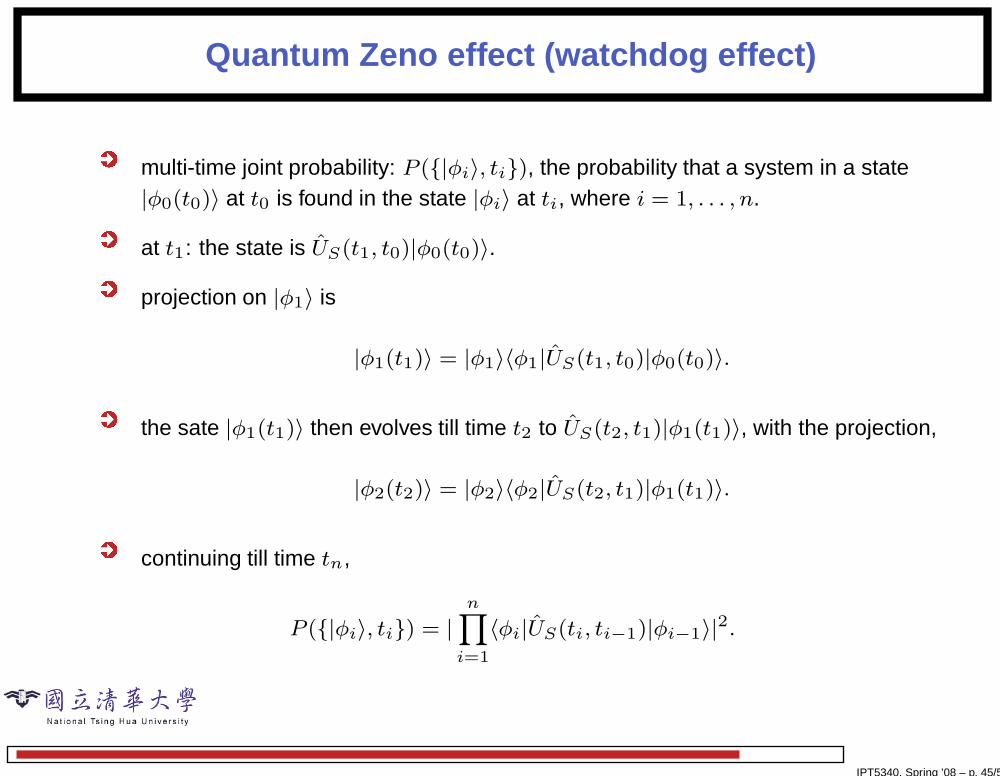
Quantum Zeno effect (watchdog effect)

multi-time joint probability: P ({|φi〉, ti}), the probability that a system in a state|φ0(t0)〉 at t0 is found in the state |φi〉 at ti, where i = 1, . . . , n.

at t1: the state is US(t1, t0)|φ0(t0)〉.

projection on |φ1〉 is

|φ1(t1)〉 = |φ1〉〈φ1|US(t1, t0)|φ0(t0)〉.

the sate |φ1(t1)〉 then evolves till time t2 to US(t2, t1)|φ1(t1)〉, with the projection,

|φ2(t2)〉 = |φ2〉〈φ2|US(t2, t1)|φ1(t1)〉.

continuing till time tn,

P ({|φi〉, ti}) = |n

Y

i=1

〈φi|US(ti, ti−1)|φi−1〉|2.

IPT5340, Spring ’08 – p. 45/51


consider a time-independent hamiltonian, US(ti, tj) = exp[−iH(ti − tj)/~].

let the observation be spaced at equal time intervals, ti − ti−1 = t/n.

the probability that at each time ti the system is observed in its initial state |φ0〉 is,

P ({|φ0〉, ti}) = |〈φ0|exp[−iHt/n~]|φ0〉|2n.

let t/n≪ 1,

|〈φ0|exp[−iHt/n~]|φ0〉|2 ≈ 1− (t

n~)2∆H2,

where ∆H2 = 〈φ0|H2|φ0〉 − 〈φ0|H|φ0〉2.

IPT5340, Spring ’08 – p. 46/51


the joint probability for n equally spaced observations becomes,

P ({|φ0〉, ti}) = [1− (t

n~)2∆H2]n.

for unobserved in between, the probability is,

P ({|φ0〉, t}) = 1− (t2

~2)∆H2.

the probability of finding the system in its initial state at a given time is increased if itis observed repeatedly at intermediate times.

for n≫ 1,

P ({|φ0〉, ti}) = [1− (t

n~)2∆H2]n ≈ exp[−t2∆H2/n~

2],

the system under observation does not evolve.

this effect was invoked to predict the inhibition of decay of an unstable system.

IPT5340, Spring ’08 – p. 47/51

Time-dependent perturbation theory

with the interaction picture, H = H0 + H1.

the state, Ψ(r, t) =P

n Cn(t)un(r)e−iωnt with the energy eigenvalueH0un(r) = ~ωnun(r).

the wavefunction has the initial value, Ψ(r, 0) = ui(r), i.e. Ci(0) = 1, Cn 6=i = 0.

the equation of motion for the probability amplitude Cn(t) is,

Cn(t) = − i~

X

m

〈n|H1|m〉eiωnmtCm(t),

≈ Cn(1)

(t) = −i~−1〈n|H1|i〉eiωnit.

if H1 = V0 time independent, we have

Cn(t) ≈ Cn(1)(t) = −i~−1〈n|H1|i〉

eiωnit − 1

iωni= −i~−1〈n|H1|i〉eiωnit/2 sin(ωnit/2)

ωni/2

Ch. 3 in ”Elements of Quantum Optics,” by P. Meystre and M. Sargent III.Ch. 5 in ”Modern Quantum Mechanics,” by J. Sakurai.

IPT5340, Spring ’08 – p. 48/51

Rotational-Wave Approximation

if H1 = V0 cos νt, we have

Cn(t) ≈ Cn(1)(t) = −i Vni

2~[ei(ωni+ν)t − 1

i(ωni + ν)+ei(ωni−ν)t − 1

i(ωni − ν)],

where Vni = 〈n|H1|i〉.

if near resonance ωni ≈ ν, we can neglect the terms with ωni + ν. This is calledthe rotational-wave approximation .

making the rotational-wave approximation,

|C(1)n |2 =

|Vni|24~2

sin2[(ωni − ν)t/2](ωni − ν)2/4

.

we have the same transition probability as the dc case, provided we substituteωni − ν for ωni.

IPT5340, Spring ’08 – p. 49/51

Fermi-Golden rule

the total transition probability from an initial state to the final state is,

PT ≈Z

D(ω)|C(1)n |2dω,

where D(ω) is the density of state factor.

Fermi-Golden rule,

PT =

Z

dωD(ω)|V (ω)|2

4~2t2

sin2[(ωni − ν)t/2][(ωni − ν)t/2]2

.

consider resonance condition ω = ν,

PT ≈ D(ν)|V (ν)|2

4~2t2

Z

dωsin2[(ωni − ν)t/2][(ωni − ν)t/2]2

,

=π

2~2D(ν)|V (ν)|2t.

the transition rate, Γ = dPTdt

= − ddt|C(1)

n |2 = π2~2

D(ν)|V (ν)|2, which is a constantin time.

IPT5340, Spring ’08 – p. 50/51

Casimir effect

IPT5340, Spring ’08 – p. 51/51

1, A brief review about Quantum Mechanics 1. Basic Quantum...

Documents

Transcript of 1, A brief review about Quantum Mechanics 1. Basic Quantum...