1

3. Random Variables

Let (, F, P) be a probability model for an experiment,

and X a function that maps every to a unique

point the set of real numbers. Since the outcome

is not certain, so is the value Thus if B is some

subset of R, we may want to determine the probability of

“ ”. To determine this probability, we can look at

the set that contains all that maps

into B under the function X.

,,Rx

.)( xX

BX )(

)(1 BXA

R)(X

x

A

B

Fig. 3.1

2

Obviously, if the set also belongs to the associated field F, then it is an event and the probability of A is well defined; in that case we can say

However, may not always belong to F for all B, thus creating difficulties. The notion of random variable (r.v) makes sure that the inverse mapping always results in an event so that we are able to determine the probability for any

Random Variable (r.v): A finite single valued function that maps the set of all experimental outcomes into the set of real numbers R is said to be a r.v, if the set is an event for every x in R.

)(1 BXA

)).((" )("event theofy Probabilit 1 BXPBX (3-1)

)(1 BX

.RB

) (X )(| xX

)( F

3

Alternatively X is said to be a r.v, if where B represents semi-definite intervals of the form and all other sets that can be constructed from these sets by performing the set operations of union, intersection and negation any number of times. The Borel collection B of such subsets of R is the smallest -field of subsets of R that includes all semi-infinite intervals of the above form. Thus if X is a r.v, then

is an event for every x. What about Are they also events ? In fact with since and are events, is an event and hence is also an event.

}{ ax

ab ? , aXbXa

bX

}{ bXabXaX aXaX c

)(| xXxX

FBX )(1

}{ aX

(3-2)

4

Thus, is an event for every n. Consequently

is also an event. All events have well defined probability. Thus the probability of the event must depend on x. Denote

The role of the subscript X in (3-4) is only to identify the actual r.v. is said to the Probability Distribution Function (PDF) associated with the r.v X.

1 aX

na

1

}{ 1

n

aXaXn

a

)(| xX

.0)( )(| xFxXP X (3-4)

)(xFX

(3-3)

5

Distribution Function: Note that a distribution function g(x) is nondecreasing, right-continuous and satisfies

i.e., if g(x) is a distribution function, then

(i)

(ii) if then

and

(iii) for all x.

We need to show that defined in (3-4) satisfies all properties in (3-6). In fact, for any r.v X,

,0)( ,1)( gg

,0)( ,1)( gg

,21 xx ),()( 21 xgxg

),()( xgxg

(3-6)

)(xFX

(3-5)

6

1)( )(| )( PXPFX

.0)( )(| )( PXPFX

(i)

and

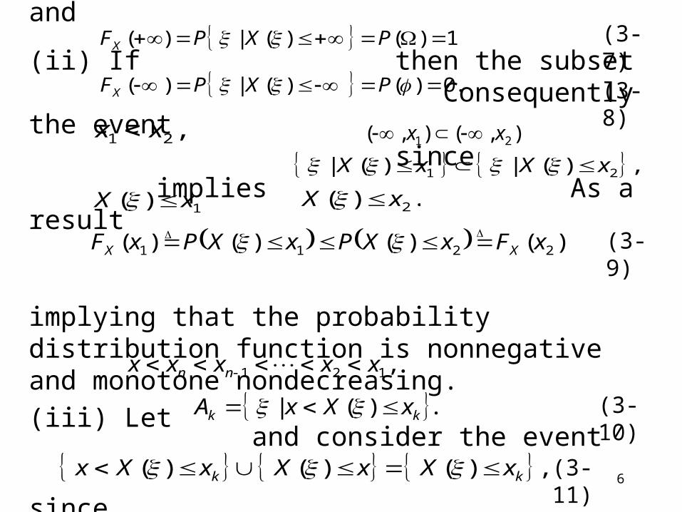
(ii) If then the subset Consequently the event since implies As a result

implying that the probability distribution function is nonnegative and monotone nondecreasing.

(iii) Let and consider the event

since

,21 xx ).,(),( 21 xx

, )(| )(| 21 xXxX

1)( xX .)( 2xX

),()()()( 2211 xFxXPxXPxF XX (3-9)

(3-7)

(3-8)

,121 xxxxx nn

.)(| kk xXxA (3-10)

, )( )( )( kk xXxXxXx (3-11)

7

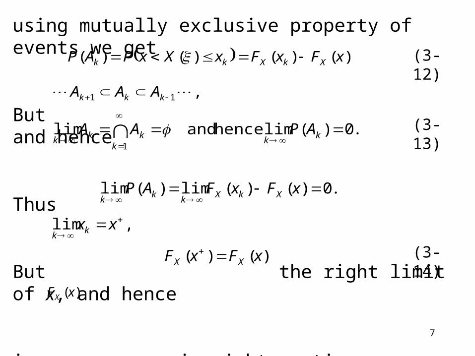
using mutually exclusive property of events we get

But and hence

Thus

But the right limit of x, and hence

i.e., is right-continuous, justifying all properties of a distribution function.

).()()()( xFxFxXxPAP XkXkk (3-12)

,11 kkk AAA

.0)(lim hence and lim1

k

kk

kkk

APAA (3-13)

.0)()(lim)(lim

xFxFAP XkXk

kk

),()( xFxF XX

)(xFX

(3-14)

,lim

xxk

k

8

Additional Properties of a PDF

(iv) If for some then

This follows, since implies is the null set, and for any will be a subset of the null set.

(v)

We have and since the two events are mutually exclusive, (16) follows.

(vi)

The events and are mutually exclusive and their union represents the event

0)( 0 xFX ,0x . ,0)( 0xxxFX (3-15)

0)()( 00 xXPxFX 0)( xX

)( ,0 xXxx

).(1 )( xFxXP X (3-16)

, )( )( xXxX

. ),()( )( 121221 xxxFxFxXxP XX (3-17)

})({ 21 xXx )( 1xX . )( 2xX

9

(vii)

Let and From (3-17)

or

According to (3-14), the limit of as from the right always exists and equals However the left limit value need not equal Thus need not be continuous from the left. At a discontinuity point of the distribution, the left and right limits are different, and from (3-20)

).()()( xFxFxXP XX (3-18)

,0 ,1 xx .2 xx

),(lim)( )( lim00

xFxFxXxP XX (3-19)

).()( )( xFxFxXP XX (3-20)

),( 0xFX )(xFX 0xx

).( 0xFX

)( 0xFX ).( 0xFX )(xFX

.0)()( )( 000 xFxFxXP XX (3-21)

10

Thus the only discontinuities of a distribution function are of the jump type, and occur at points where (3-21) is satisfied. These points can always be enumerated as a sequence, and moreover they are at most countable in number. Example 3.1: X is a r.v such that Find Solution: For so that and for so that (Fig.3.2)

Example 3.2: Toss a coin. Suppose the r.v X is such that Find

)(xFX

0x

. ,)( cX ).(xFX

, )( , xXcx ,0)( xFX

.,TH.1)( ,0)( HXTX

)(xFX

xc

1

Fig. 3.2

).(xFX

.1)( xFX ,)( , xXcx

11

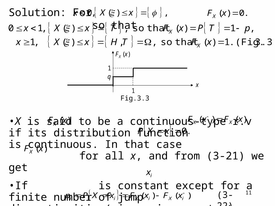
Solution: For so that

•X is said to be a continuous-type r.v if its distribution function is continuous. In that case for all x, and from (3-21) we get

•If is constant except for a finite number of jump discontinuities(piece-wise constant; step-type), then X is said to be a discrete-type r.v. If is such a discontinuity point, then from (3-21)

, )( ,0 xXx .0)( xFX

3.3) (Fig. .1)( that so , , )( ,1

,1 )( that so , )( ,10

xFTHxXx

pTPxFTxXx

X

X

).()( iXiXii xFxFxXPp (3-22)

)(xFX)()( xFxF XX

.0xXP

)(xFX

)(xFX

x

Fig.3.3

1q

1

ix

12

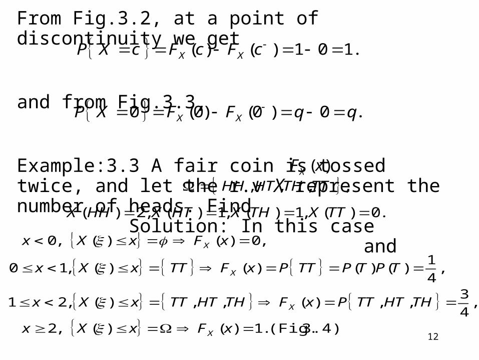
From Fig.3.2, at a point of discontinuity we get

and from Fig.3.3,

Example:3.3 A fair coin is tossed twice, and let the r.v X represent the number of heads. Find Solution: In this case and

.101)()( cFcFcXP XX

.0)0()0( 0 qqFFXP XX

, ,,, TTTHHTHH).(xFX

.0)(,1)(,1)(,2)( TTXTHXHTXHHX

3.4) (Fig. .1)()( ,2

,4

3,, )(,, )( ,21

,4

1)()( )( )( ,10

,0)()( ,0

xFxXx

THHTTTPxFTHHTTTxXx

TPTPTTPxFTTxXx

xFxXx

X

X

X

X

13

From Fig.3.4,

Probability density function (p.d.f)

The derivative of the distribution function is called the probability density function of the r.v X. Thus

Since

from the monotone-nondecreasing nature of

.2/14/14/3)1()1(1 XX FFXP

)(xFX

)(xf X

.

)()(

dx

xdFxf X

X

,0)()(

lim

)(0

x

xFxxF

dx

xdF XX

x

X

(3-23)

(3-24)

),(xFX

)(xFX

x

Fig. 3.4

1

4/1

1

4/3

2

14

it follows that for all x. will be a continuous function, if X is a continuous type r.v. However, if X is a discrete type r.v as in (3-22), then its p.d.f has the general form (Fig. 3.5)

where represent the jump-discontinuity points in As Fig. 3.5 shows represents a collection of positive discrete masses, and it is known as the probability mass function (p.m.f ) in the discrete case. From (3-23), we also obtain by integration

Since (3-26) yields

0)( xf X )(xf X

,)()( i

iiX xxpxf

).(xFX

(3-25)

.)()( duufxFx

xX (3-26)

,1)( XF

,1)(

dxxf x

(3-27)

ix

)(xf X

xix

ip

Fig. 3.5

)(xf X

15

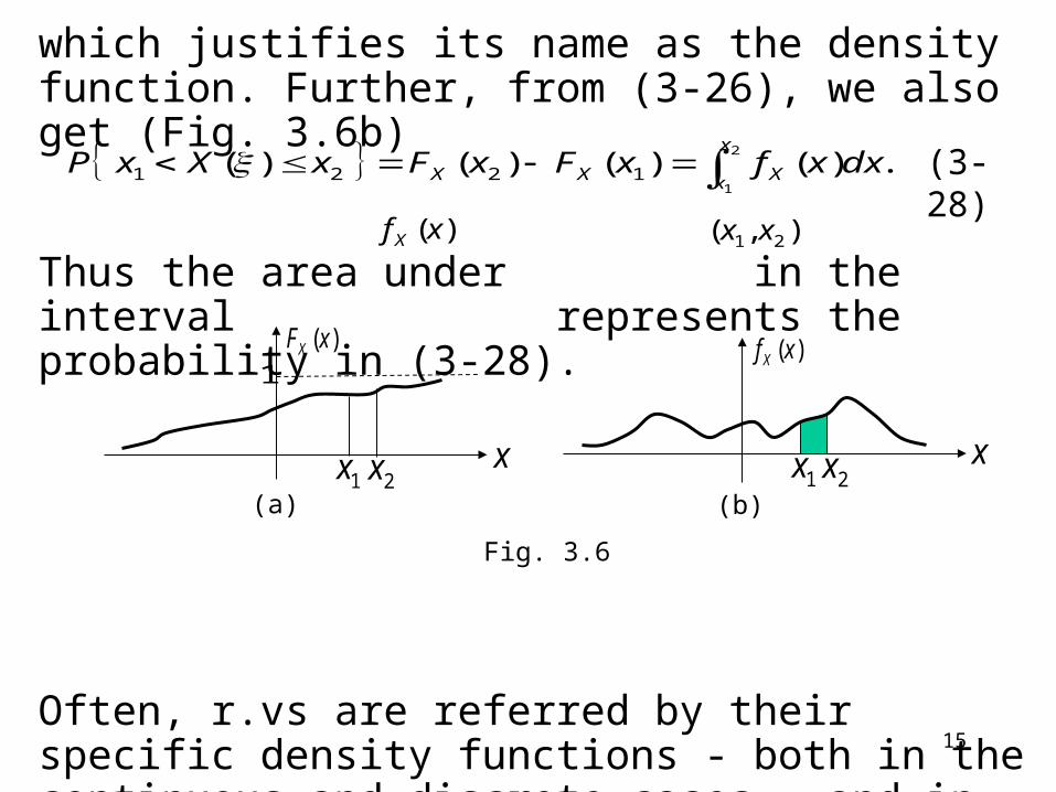
which justifies its name as the density function. Further, from (3-26), we also get (Fig. 3.6b)

Thus the area under in the interval represents the probability in (3-28).

Often, r.vs are referred by their specific density functions - both in the continuous and discrete cases - and in what follows we shall list a number of them in each category.

.)()()( )( 2

11221 dxxfxFxFxXxP

x

x XXX (3-28)

Fig. 3.6

)(xf X ),( 21 xx

)(xf X

(b)

x1x 2x

)(xFX

x

1

(a)1x 2x

16

Continuous-type random variables

1. Normal (Gaussian): X is said to be normal or Gaussian r.v, if

This is a bell shaped curve, symmetric around the parameter and its distribution function is given by

where is often tabulated. Since depends on two parameters and the notation will be used to represent (3-29).

.2

1)(

22 2/)(

2

x

X exf (3-29)

,

,2

1)(

22 2/)(

2

x y

X

xGdyexF

(3-30)

dyexG yx 2/2

2

1)(

),( 2NX)(xf X

xFig. 3.7

)(xf X

,2

17

2. Uniform: if (Fig. 3.8), ),,( babaUX

otherwise. 0,

, ,1

)( bxaabxf X

(3.31)

)(xf X

xa b

ab 1

Fig. 3.8

3. Exponential: if (Fig. 3.9))( X

otherwise. 0,

,0 ,1

)(/ xexf

x

X

(3-32)

)(xf X

x

Fig. 3.9

18

4. Gamma: if (Fig. 3.10)

If an integer

5. Beta: if (Fig. 3.11)

where the Beta function is defined as

),( GX )0 ,0(

otherwise. 0,

,0 ,)()(

/1

xex

xfx

X

(3-33)

n )!.1()( nn

),( baX )0 ,0( ba

otherwise. 0,

,10 ,)1(),(

1)(

11 xxxbaxf

ba

X (3-34)

),( ba

1

0

11 .)1(),( duuuba ba (3-35)

x

)(xf X

x

Fig. 3.11

10

)(xf X

Fig. 3.10

19

6. Chi-Square: if (Fig. 3.12)

Note that is the same as Gamma

7. Rayleigh: if (Fig. 3.13)

8. Nakagami – m distribution:

),( 2 nX

)(2 n ).2 ,2/(n

otherwise. 0,

,0 ,)(22 2/

2xe

xxf

x

X

(3-36)

(3-37)

,)( 2RX

x

)(xf X

Fig. 3.12

)(xf X

xFig. 3.13

otherwise. 0,

,0 ,)2/(2

1)(

2/12/2/

xexnxf

xnn

X

22 1 /2, 0

( ) ( )

0 otherwiseX

mm mxm

x e xf x m

(3-38)

20

9. Cauchy: if (Fig. 3.14)

10. Laplace: (Fig. 3.15)

11. Student’s t-distribution with n degrees of freedom (Fig 3.16)

. ,1

)2/(

2/)1()(

2/)1(2

tn

t

nn

ntf

n

T

,),( CX

. ,)(

/)(

22

x

xxf X

. ,2

1)( /|| xexf x

X

)(xf X

x

Fig. 3.14

(3-41)

(3-40)

(3-39)

x

)(xf X

Fig. 3.15

t

( )T

f t

Fig. 3.16

21

12. Fisher’s F-distribution/ 2 / 2 / 2 1

( ) / 2

{( ) / 2} , 0

( ) ( / 2) ( / 2) ( )

0 otherwise

m n m

m nz

m n m n zz

f z m n n mz

(3-42)

22

Discrete-type random variables

1. Bernoulli: X takes the values (0,1), and

2. Binomial: if (Fig. 3.17)

3. Poisson: if (Fig. 3.18)

.)1( ,)0( pXPqXP (3-43)

),,( pnBX

.,,2,1,0 ,)( nkqpk

nkXP knk

(3-44)

, )( PX

.,,2,1,0 ,!

)( kk

ekXPk

(3-45)

k

)( kXP

Fig. 3.17

12 n

)( kXP

Fig. 3.18

23

4. Hypergeometric:

5. Geometric: if

6. Negative Binomial: ~ if

7. Discrete-Uniform:

(3-49)

(3-48)

(3-47)

.,,2,1 ,1

)( NkN

kXP

),,( prNBX1

( ) , , 1, .1

r k rkP X k p q k r r

r

.1 ,,,2,1,0 ,)( pqkpqkXP k

)( pgX

, max(0, ) min( , )( )

m N m

k n kN

n

m n N k m nP X k

(3-46)