The ECCO Report Series 1

The Global Ocean State During 1992 {1997,

Estimated from Ocean observations and a General

Circulation Model

Part III:

Volume, Heat and Freshwater Transports

D. Stammer2, C. Wunsch3, R. Giering4 C. Eckert2, P. Heimbach2,

J. Marotzke5, A. Adcroft2, C.N. Hill2, and J. Marshall2

Na tional Oceanographic Partn

ershipPro

gra

m

Estim

ating the Circ

ulation and Climate of the Ocean

Report Number 6

Submitted to Journal of Geophysical Research

August 24, 2001.

1The ECCO Project is funded through a grant from the National Oceanographic Partnership Program(NOPP).

2Copies of this Report are available at www.ecco-group.org or from Detlef Stammer, Scripps Insti-tution of Oceanography, La Jolla CA 92093-0230, ph.: (858) 822-3376; fax: (858) 534-4464; e-mail:dstammer@ucsd.edu

3Massachusetts Institute of Technology4FastOpt, GBR, Hamburg5Southampton Oceanographic Center

Abstract

An analysis of ocean volume, heat and freshwater transports from a fully con-

strained general circulation model is described. Output from a data synthesis, or

state estimation, method is used by which the model was forced to a large-scale, time

varying global ocean data set over six years. Time-mean uxes estimated from this

fully time-dependent circulation have converged with independent time-independent

estimates from box inversions over most parts of the world ocean but especially in

the southern hemisphere. However, heat transport estimates di�er substantially in

the North Atlantic where our estimates result in only 1/2 previous heat transports.

The estimated mean circulation around Australia involves a net volume ux of 14

Sv through the Indonesian Through ow and the Mozambique Channel. In addition

we show that this ow regime exist on all time scales above one month rendering the

variability in the South Paci�c strongly coupled to the Indian Ocean. Moreover,

the dynamically consistent variations in the model show temporal variability of

oceanic heat uxes, heat storage and atmospheric exchanges that are complex and

with a strong dependence upon location, depth, and time-scale. Results presented

demonstrate the great potential of an ocean /state estimation system to provide

a dynamical description of the time-dependent observed heat transport and heat

content changes and their relation to air-sea interactions.

1

1 Introduction

One of the purposes of the World Ocean Circulation Experiment (WOCE) has been to

achieve a full synthesis of the global observations to determine the general circulation and

its transport variability over an extended period. This goal can be reached by bringing

a full ocean circulation model into consistency with the diverse ocean observations and

using the combination to study the circulation, its energetics, driving forces, property

uxes, dynamical balances, and the nature and structure of its variability, among many

other problems.

In a previous paper (Stammer et al., 2001a, hereafter Paper 1), we described the over-

all results from an initial attempt at a combination of a general circulation model (GCM)

with much of the existing global data from a six year interval 1992 { 1997, in a procedure

called \state estimation" or \data assimilation". In contrast to a number of other such at-

tempts (e.g., Carton et al., 2000a,b), a deliberate decision was made to use a very general

method|one that could become rigorous as computer power grows and as knowledge of

the underlying statistics improves|at the expense of a greater computational load. Im-

posed data included both mean and time-varying altimetry, hydrographic climatologies,

as well as the estimated air-sea uxes of momentum, fresh water and heat from twice-daily

atmospheric estimates. Paper 1 provides details of the method (Lagrange multipliers, or

adjoint), the optimization and some general tests of the adequacy of the model-data com-

bination. In particular, it shows that the constrained model displays considerable skill in

reproducing both the observations, and much of the withheld data. Remaining discrep-

ancies can lie with either the model, the data, or both, and require further information to

resolve. Despite various lingering issues, an overall conclusion was that the constrained

model displays considerable skill in reproducing the observations, and in particular with

qualitative and quantitative features of the withheld data. We therefore begin here to

exploit the results for scienti�c purposes.

Our focus is on the determination of the ocean uxes of volume, heat and freshwater

and their divergences that appear to be most important to understanding the climate

system. Because the �rst year of the optimization shows some residual signs of adjustment

2

problems, we base the following analysis on the last �ve years of the optimized estimate.

A more detailed analysis of associated surface heat, freshwater, and momentum uxes and

their uncertainties will be described elsewhere (Stammer et al., 2001b). Because of: (1)

the nature of the T/P data set which best constrains the time variability on time scales

out to about �ve years, and (2) concerns about adequate model resolution, we believe

that the temporal variability of properties in our results is considerably more accurate

than is the time average or absolute values. Thus, while we describe the time average

results, most of our emphasis will be on discussing the uctuating components.

In the absence so far, because of the computational load, of a formal full error analysis

of the estimated ocean state, comparisons with independent estimates of various quan-

tities are used to build up an empirical depiction of the overall accuracy of the results.

Obtaining realistic property uxes, such as those for temperature, puts stringent demands

on a model: the transports are second-order quantities, involving products of velocities

and property distributions; models that produce sensible-appearing ow and temperature

�elds may well fail to estimate accurately integrated products of these �elds.

The results reported are believed to be the �rst obtained from a general circulation

model whose quantitative consistency with complete global data sets has been enforced

in a dynamically consistent way. More applications exist than the one described here;

for example, Ponte et al. (2001), used the same results to study the Earth's angular

momentum balance, and e�orts to calculate the corresponding biogeochemical uxes are

underway.

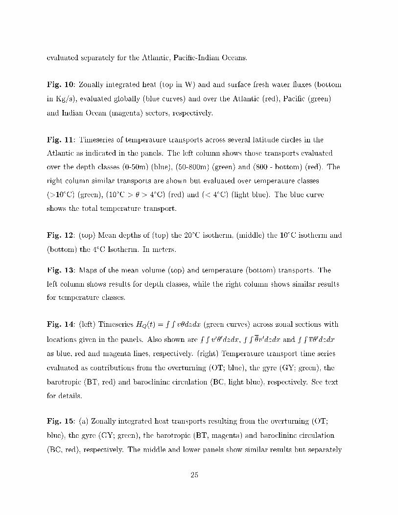
An indication of the skill of the present analysis can be found in Fig. 1 which depicts Fig. 1

the depth of the 20ÆC isotherm as measured from six years of TOGA-TAO (Tropical Ocean

Global Atmosphere-Tropical-Atmosphere-Ocean) measurements (McPhaden et al., 1998)

on the equator between (140Æ-150ÆE) and at 265ÆE. Despite gaps, one sees the clear signal

of the 1992/93, 1994/95 and the 1997 Ni~nos events. Also shown are the respective results

from the unconstrained and constrained models. While the unconstrained model produces

a fairly constant isotherm depth in the west, and loses the warm water altogether in the

east, the constrained result shows much better agreement with the observations. The

model skill illustrated in the �gure is noteworthy given the low resolution of the model

3

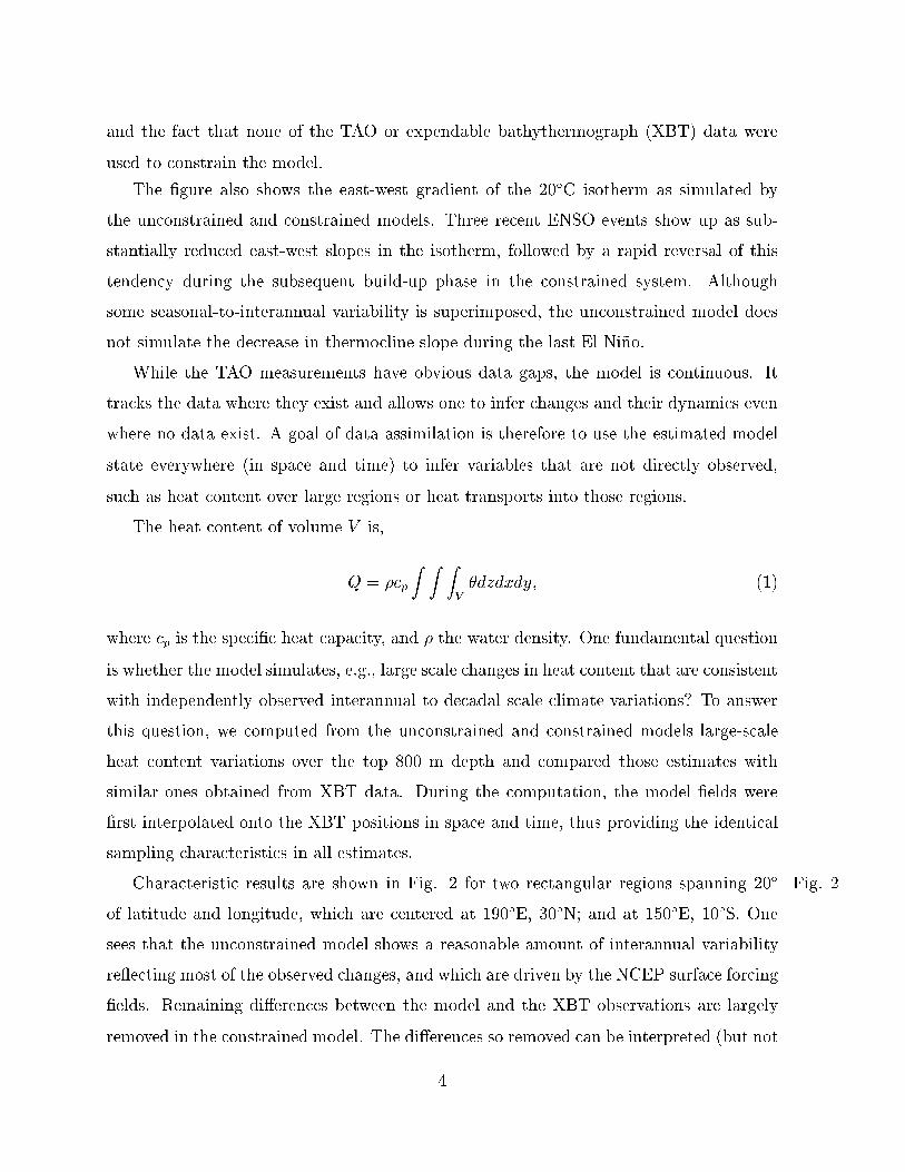
and the fact that none of the TAO or expendable bathythermograph (XBT) data were

used to constrain the model.

The �gure also shows the east-west gradient of the 20ÆC isotherm as simulated by

the unconstrained and constrained models. Three recent ENSO events show up as sub-

stantially reduced east-west slopes in the isotherm, followed by a rapid reversal of this

tendency during the subsequent build-up phase in the constrained system. Although

some seasonal-to-interannual variability is superimposed, the unconstrained model does

not simulate the decrease in thermocline slope during the last El Ni~no.

While the TAO measurements have obvious data gaps, the model is continuous. It

tracks the data where they exist and allows one to infer changes and their dynamics even

where no data exist. A goal of data assimilation is therefore to use the estimated model

state everywhere (in space and time) to infer variables that are not directly observed,

such as heat content over large regions or heat transports into those regions.

The heat content of volume V is,

Q = �cp

Z Z ZV�dzdxdy; (1)

where cp is the speci�c heat capacity, and � the water density. One fundamental question

is whether the model simulates, e.g., large scale changes in heat content that are consistent

with independently observed interannual to decadal scale climate variations? To answer

this question, we computed from the unconstrained and constrained models large-scale

heat content variations over the top 800 m depth and compared those estimates with

similar ones obtained from XBT data. During the computation, the model �elds were

�rst interpolated onto the XBT positions in space and time, thus providing the identical

sampling characteristics in all estimates.

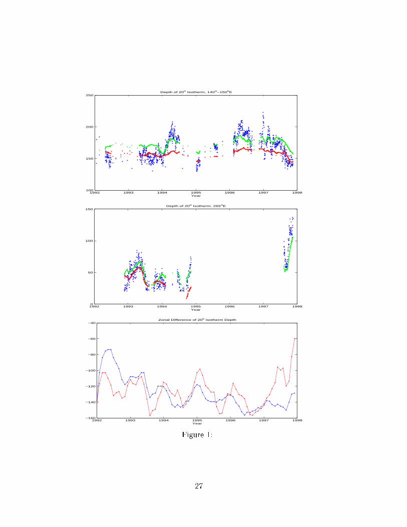
Characteristic results are shown in Fig. 2 for two rectangular regions spanning 20Æ Fig. 2

of latitude and longitude, which are centered at 190ÆE, 30ÆN; and at 150ÆE, 10ÆS. One

sees that the unconstrained model shows a reasonable amount of interannual variability

re ecting most of the observed changes, and which are driven by the NCEP surface forcing

�elds. Remaining di�erences between the model and the XBT observations are largely

removed in the constrained model. The di�erences so removed can be interpreted (but not

4

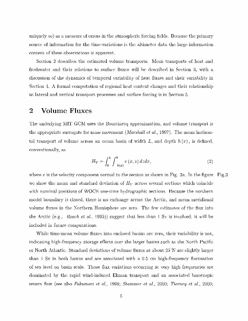
uniquely so) as a measure of errors in the atmospheric forcing �elds. Because the primary

source of information for the time-variations is the altimeter data the large information

content of these observations is apparent.

Section 2 describes the estimated volume transports. Mean transports of heat and

freshwater and their relations to surface uxes will be described in Section 3, with a

discussion of the dynamics of temporal variability of heat uxes and their variability in

Section 4. A formal computation of regional heat content changes and their relationship

to lateral and vertical transport processes and surface forcing is in Section 5.

2 Volume Fluxes

The underlying MIT GCM uses the Boussinesq approximation, and volume transport is

the appropriate surrogate for mass movement (Marshall et al., 1997). The mean horizon-

tal transport of volume across an ocean basin of width L; and depth h (x) ; is de�ned,

conventionally, as

HV =Z L

0

Z 0

�h(x)v (x; z) dzdx; (2)

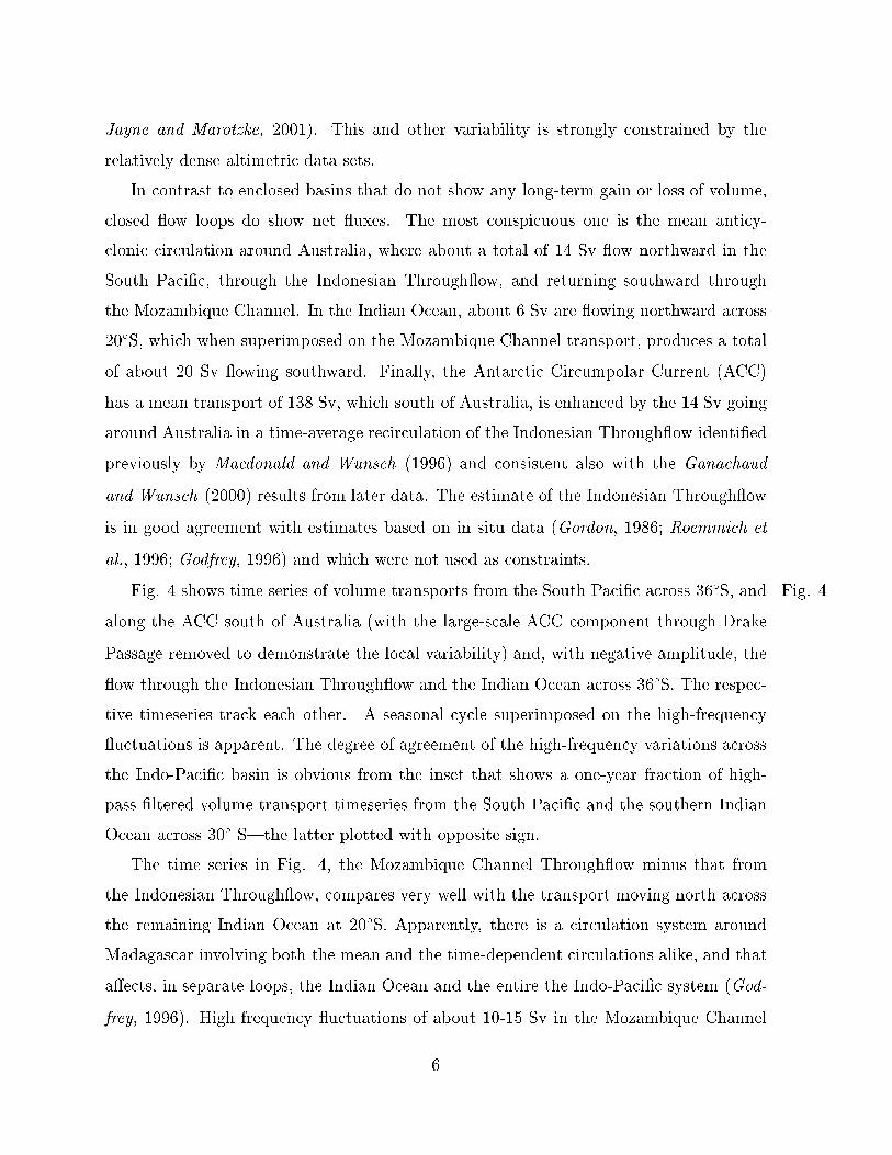
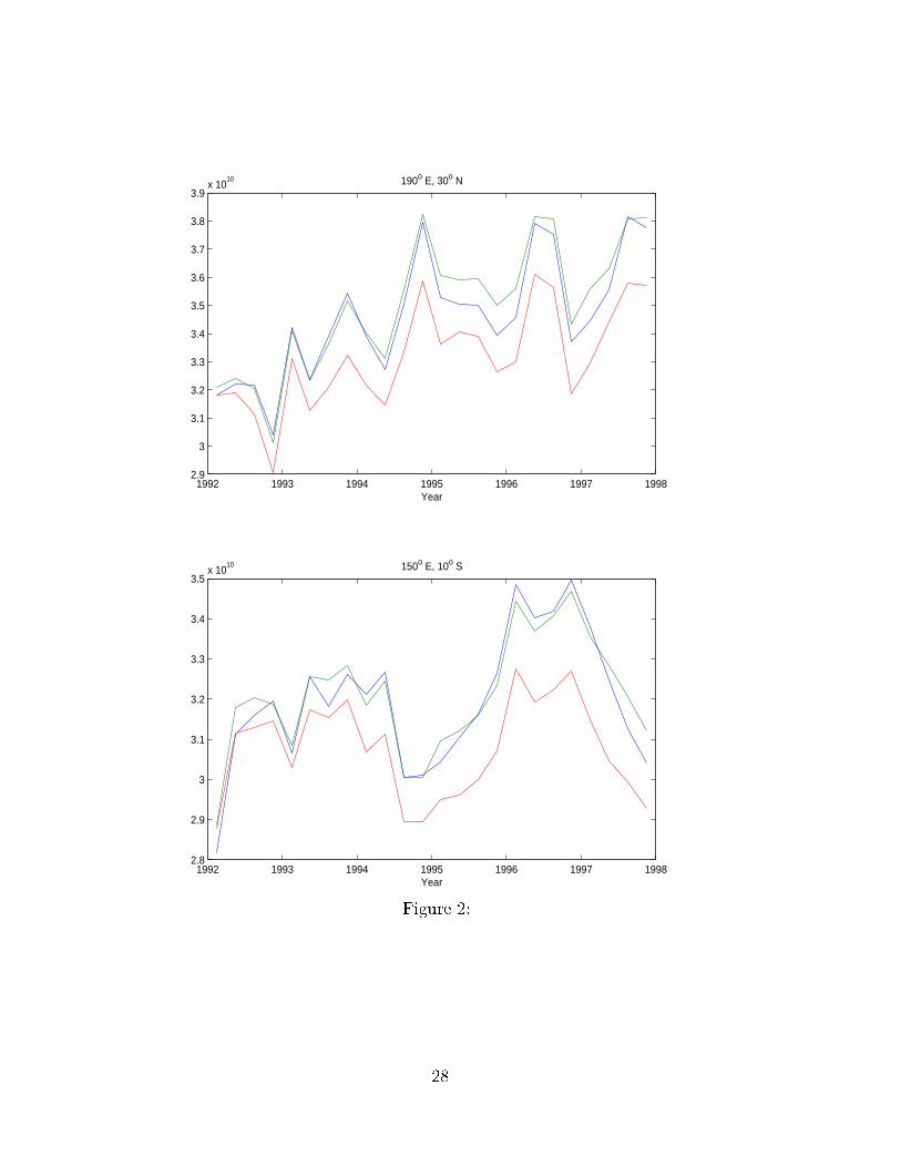
where v is the velocity component normal to the section as shown in Fig. 3a. In the �gure Fig.3

we show the mean and standard deviation of HV across several sections which coincide

with nominal positions of WOCE one-time hydrographic sections. Because the northern

model boundary is closed, there is no exchange across the Arctic, and mean meridional

volume uxes in the Northern Hemisphere are zero. The few estimates of the ux into

the Arctic (e.g., Roach et al., 1995)) suggest that less than 1 Sv is involved; it will be

included in future computations.

While time-mean volume uxes into enclosed basins are zero, their variability is not,

indicating high-frequency storage e�ects over the larger basins such as the North Paci�c

or North Atlantic. Standard deviations of volume uxes at about 25ÆN are slightly larger

than 1 Sv in both basins and are associated with a 0.5 cm high-frequency uctuation

of sea level on basin scale. Those ux variations occurring at very high frequencies are

dominated by the rapid wind-induced Ekman transport and an associated barotropic

return ow (see also Fukumori et al., 1998; Stammer et al., 2000; Tierney et al., 2000;

5

Jayne and Marotzke, 2001). This and other variability is strongly constrained by the

relatively dense altimetric data sets.

In contrast to enclosed basins that do not show any long-term gain or loss of volume,

closed ow loops do show net uxes. The most conspicuous one is the mean anticy-

clonic circulation around Australia, where about a total of 14 Sv ow northward in the

South Paci�c, through the Indonesian Through ow, and returning southward through

the Mozambique Channel. In the Indian Ocean, about 6 Sv are owing northward across

20ÆS, which when superimposed on the Mozambique Channel transport, produces a total

of about 20 Sv owing southward. Finally, the Antarctic Circumpolar Current (ACC)

has a mean transport of 138 Sv, which south of Australia, is enhanced by the 14 Sv going

around Australia in a time-average recirculation of the Indonesian Through ow identi�ed

previously by Macdonald and Wunsch (1996) and consistent also with the Ganachaud

and Wunsch (2000) results from later data. The estimate of the Indonesian Through ow

is in good agreement with estimates based on in situ data (Gordon, 1986; Roemmich et

al., 1996; Godfrey, 1996) and which were not used as constraints.

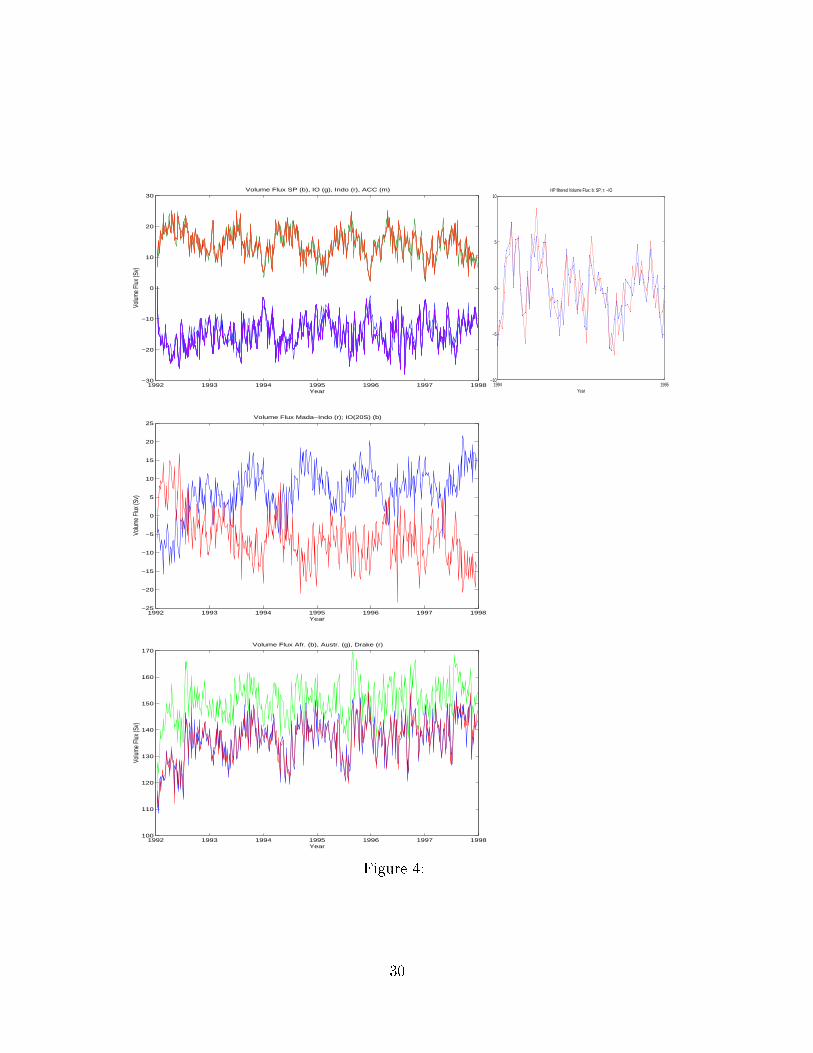
Fig. 4 shows time series of volume transports from the South Paci�c across 36ÆS, and Fig. 4

along the ACC south of Australia (with the large-scale ACC component through Drake

Passage removed to demonstrate the local variability) and, with negative amplitude, the

ow through the Indonesian Through ow and the Indian Ocean across 36ÆS. The respec-

tive timeseries track each other. A seasonal cycle superimposed on the high-frequency

uctuations is apparent. The degree of agreement of the high-frequency variations across

the Indo-Paci�c basin is obvious from the inset that shows a one-year fraction of high-

pass �ltered volume transport timeseries from the South Paci�c and the southern Indian

Ocean across 30Æ S|the latter plotted with opposite sign.

The time series in Fig. 4, the Mozambique Channel Through ow minus that from

the Indonesian Through ow, compares very well with the transport moving north across

the remaining Indian Ocean at 20ÆS. Apparently, there is a circulation system around

Madagascar involving both the mean and the time-dependent circulations alike, and that

a�ects, in separate loops, the Indian Ocean and the entire the Indo-Paci�c system (God-

frey, 1996). High frequency uctuations of about 10-15 Sv in the Mozambique Channel

6

have a net standard deviation of about 5 Sv. The ACC south of Africa, Australia, and

through Drake Passage, shows a strong seasonal cycle superimposed on high-frequency

uctuations. Near Australia, the additional, largely high-frequency variability seen in the

Mozambique Channel characterizing the Indo-Paci�c closed loop circulation, is superim-

posed on the ACC transport variability.

Various previous estimates of the ACC transport exist. For example, Whitworth

(1983), using a combination of moorings and hydrographic surveys, estimated a range

of 118-146 Sv, with a mean of 121 Sv through the Drake Passage, but subject to various

sampling errors. Nowlin and Klink (1986) report 135 � 5 Sv in good agreement with

our results. As with the other sections, results for the ACC show that reports of \mean"

volume transports from �eld programs of duration of a year or shorter cannot and should

not be interpreted as representing the long-term average. In particular, the Indonesian

Through ow and Drake Passage uxes would require many years of averaging to produce

a stable mean (and the model underestimates the high frequency variability owing to the

absence of eddies and related motions).

Fig. 4 shows that in the model, the South-Paci�c Indian Ocean system is spinning

down in the sense that the northward transport and its return in the Indian Ocean is

weakening by almost 5 Sv. over the six years. At the same time the ACC transport

is strengthening steadily over the entire period. Note also that the Indian Ocean shows

almost no net northward volume ux during boreal winter, and a maximum of around 10

Sv between October and December.

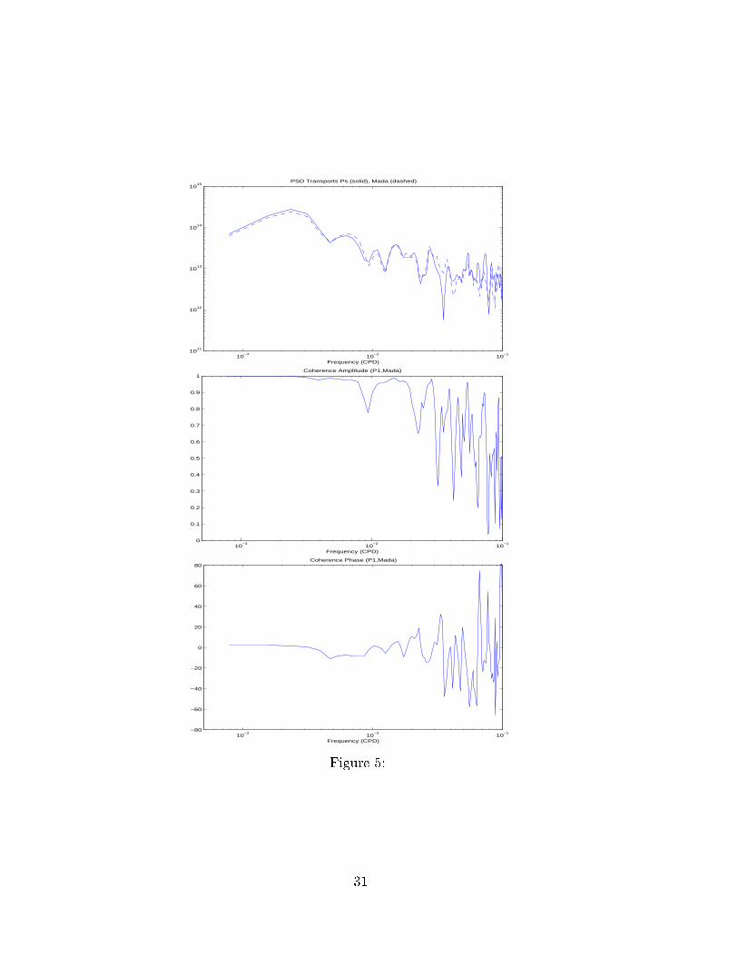
Fig. 5a shows a spectral estimate of the transport across 20ÆS in the Paci�c and Fig. 5

compares it with a similar estimate from the Mozambique Channel minus the transport

across the remaining Indian Ocean at this latitude. The results and their coherence

(Fig. 5b) are consistent with the visual impression that the variations in both records

are almost identical at periods longer than about �fty days at zero phase. (Fig. 5c).

The causes of this large scale variation have not been established, but are conjectured

to be a combination of directly forced large-scale wind-driven motions and a dominantly

barotropic response. Such large scale motions demonstrate the connected nature of the

ocean circulation and its variability, and underline the need to study it on a global basis.

7

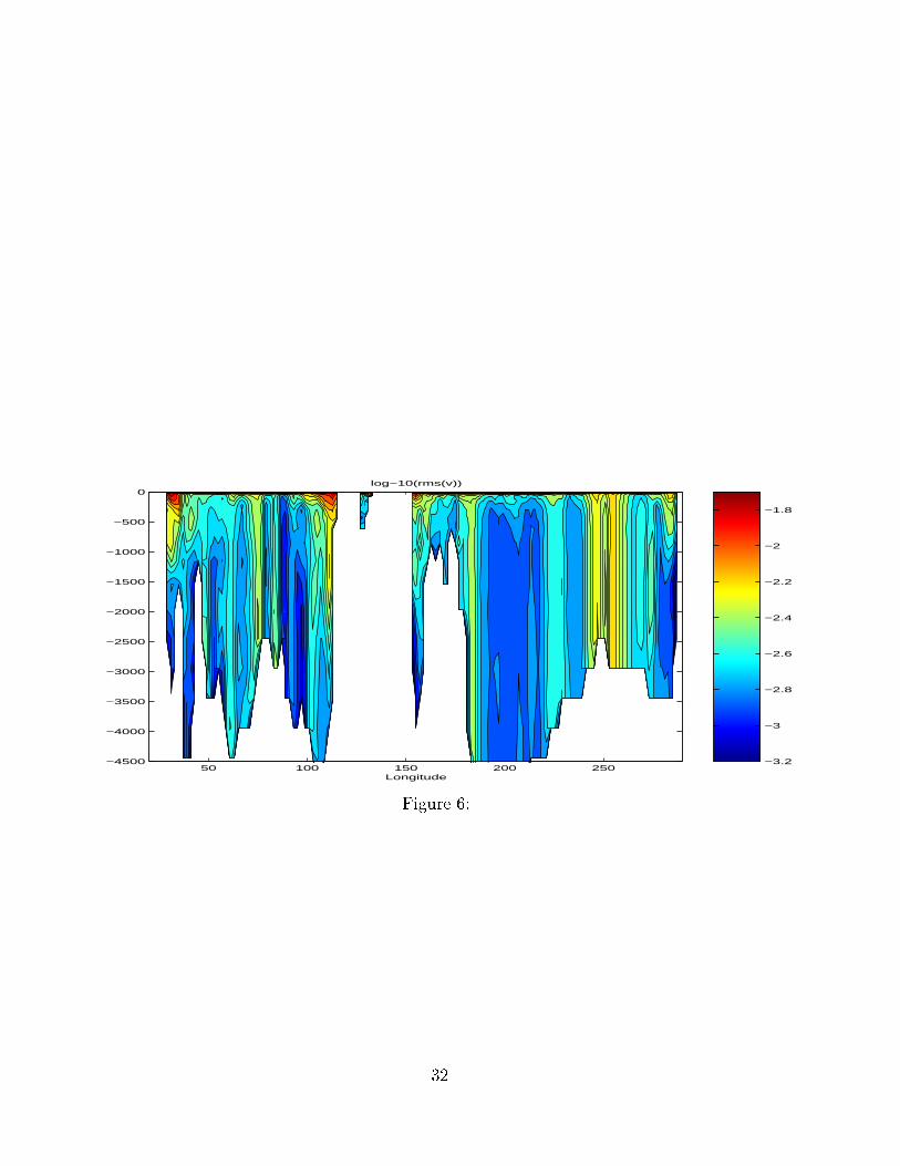
Volume ux variability is of course, not uniformly distributed along the sections. As

one example, Fig. 6 shows the logarithm of the standard deviation of volume ux along Fig. 6

31ÆS. High variability is associated primarily with shallow boundary currents on both

sides of the Indian and Paci�c Oceans. However, enhanced variability in the northward

velocity component can also be seen along the anks of most steep topographic features in

the model, notably the Ninetyeast Ridge in the central Indian Ocean and the East-Paci�c

Rise. Note that the latter was previously identi�ed as a region of vigorous barotropic

variability (e.g., Fukumori et al. 1998; Stammer et al., 2000). A similar feature appears

in the Indian Ocean sector of the �gure, although with reduced amplitude.

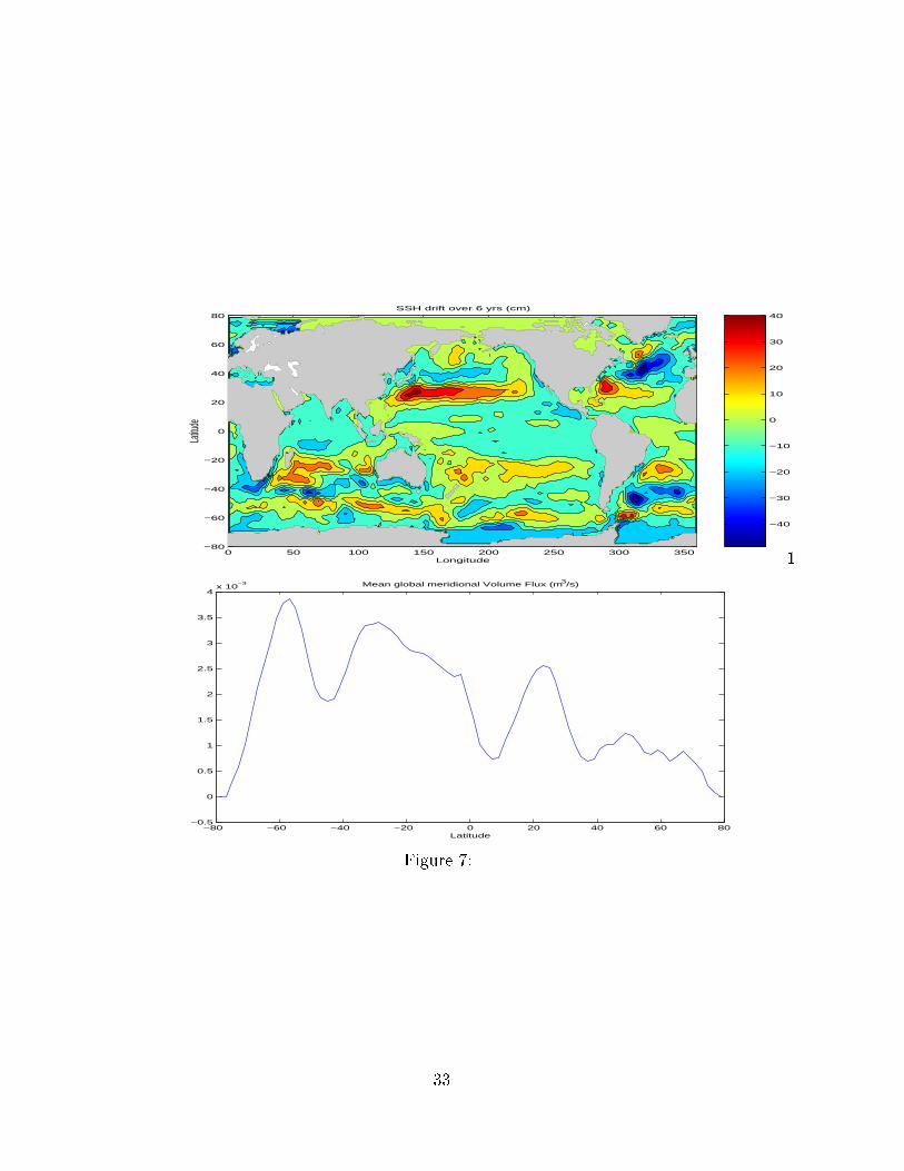
The trends in volume transport (Fig. 4) indicate a remaining overall mass adjustment

occurring in the model. This adjustment is displayed in a more complete way in Fig. 7

showing the mean changes in sea surface height over the six year period. The largest Fig. 7

changes are of the order of � 20 cm and can be found over the subtropical gyres of the

northern hemisphere. Smaller changes are visible across the model ACC. The associated

mean southward volume ux is obtained by averaging the model meridional ow over the

entire globe. Results are consistent with the changes in sea surface height and indicate

adjustments of the order of 10�3 Sv. The values are approximately the same as seen

in TOPEX/POSEIDON global and regional trend data (Nerem et al., 1999; F. Condi

personal communication, 2000) and demonstrate one of the diÆculties encountered in

explaining global sealevel rise in the presence of numerical model drift.

3 Mean Heat and Freshwater Fluxes

The time rate of change of a heat content Q, de�ned in (1) is,

@Q

@t= �r � FQ +HQ; (3)

where HQ is the surface net heat ux and the zonally integrated meridional transports of

temperature is

FQ = �cp

Z L

0

Z 0

�Hv�dzdx: (4)

8

(see Bohren and Albrecht, 1998 or Warren, 2000, for a discussion of the meaning of

\heat transport", which we will nonetheless continue to use as a shorthand for \energy

transport").

Time mean values of FQ in the model across various WOCE sections and their stan-

dard deviation are shown in Fig. 4b. In the present solution, there is a mean temperature

ux of about 1.3 PW from the Paci�c into the Indian Ocean. Most of this heat then

moves southward through the Mozambique Channel. In contrast to the volume ux, the

entire Indian Ocean shows southward temperature ux at the latitude of Mozambique.

Some of it is communicated to the atmosphere between 20ÆS and 36ÆS and about 1 PW is

being released into the ACC region. Note that in our estimate, the 0.25 PW transported

from the Indo-Paci�c system into the Atlantic follows the \cold-water route" through the

Drake Passage (see Gordon, 1986; Rintoul, 1991Macdonald, 1998; Ganachaud and Wun-

sch, 2000). This total dominance by the cold-water route may be a consequence of the

absence of any eddy variability or Agulhas ring formation in the coarse-resolution model.

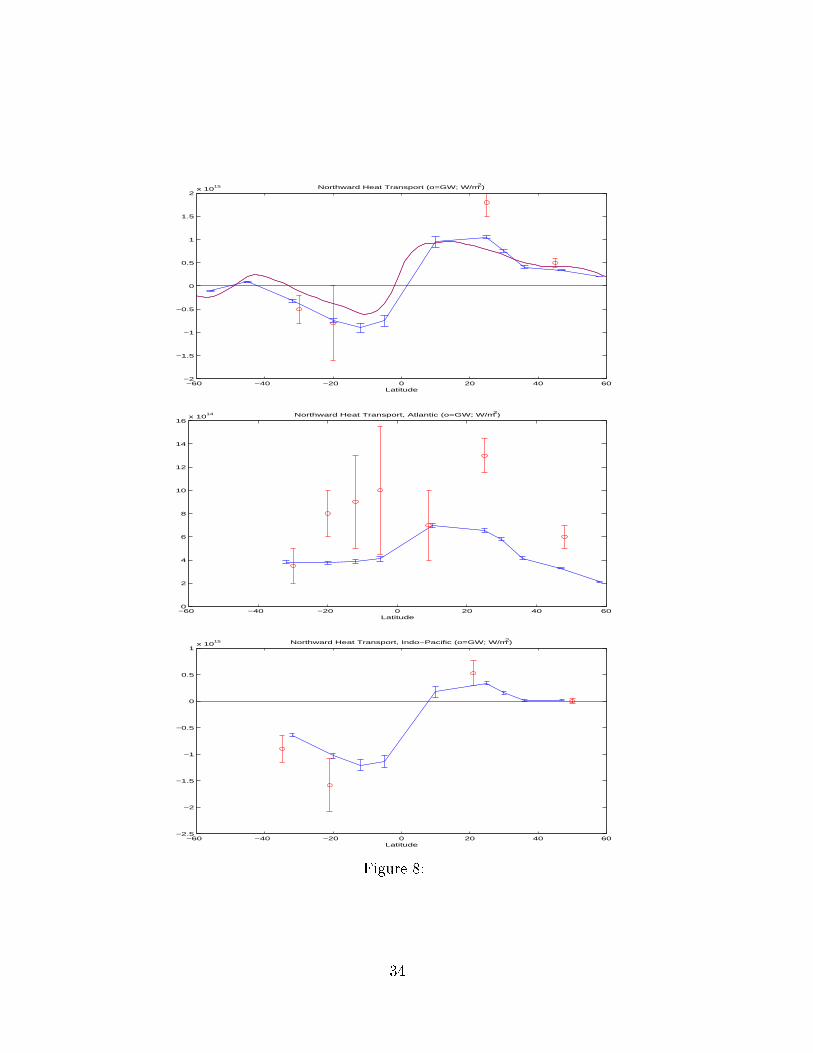
Fig. 8 shows zonally integrated meridional heat uxes and separately for the Atlantic Fig. 8

and Paci�c-Indian Oceans. Also shown are error bars estimated as �=pN from the

temporal standard deviations �, with N being the number of degrees-of-freedom, taken

here to be approximately 435|the number of individual 5-day estimates. The green open

circles show the zonal integrals as obtained by Ganachaud and Wunsch (2000). Although

our estimates agree with theirs surprisingly well in the Southern Hemisphere and in the

North Paci�c, large discrepancies exist over the Atlantic where we estimate only about

50% of their amplitude, except at 10ÆN and at the southern end of the picture. However,

this result is unsurprising in a 2Æ lateral resolution model in which the boundary currents

are sluggish and di�use, with the data unable to impose a di�erent, sharper, spatial

structure. Despite this resolution problem, the gross pattern of North Atlantic poleward

heat ux is reproduced and its dependence on the closed nature of the poleward model

boundaries or other model parameters has to be investigated. See Stammer et al. (2001b)

for a further discussion.

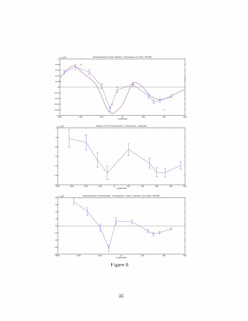
In Fig. 9 we show the zonally integrated meridional freshwater transports and their Fig. 9

9

standard deviation, estimated as

FW =Z Z 0

�H�v(1� S)dzdx: (5)

Freshwater ux estimates are in turn very similar toWij�els et al. (1992) over most parts

of the ocean.

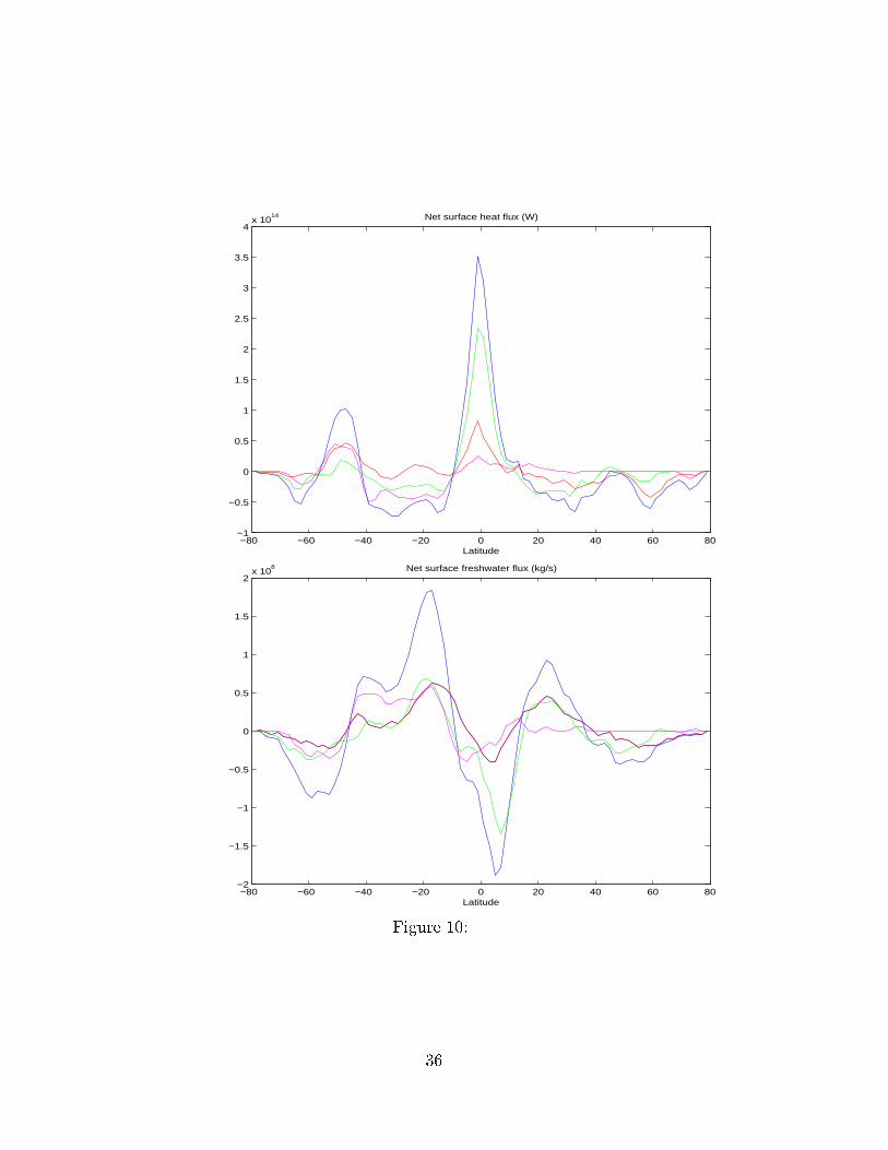
Basin-integrated net surface heat and freshwater uxes, corresponding to the diver-

gences of the meridional uxes in Figs. 8 and 9, are shown in Fig. 10 evaluated here from Fig. 10

the estimated surface net heat and freshwater ux �elds displayed in Paper 1. Both global

integrals, and those for individual basins are shown. Heat ux in the Northern Hemisphere

outside the tropics is negative, that is, the ocean loses heat to the atmosphere. A similar

result appears in the Southern Hemisphere between 10Æ and 40ÆS. The Southern Ocean,

however, shows a pronounced warming pattern with net amplitude close to 1/3 of that of

the tropical ocean. This warming is mostly located over the Atlantic and Indian sectors

of the ACC, again consistent with the Ganachaud and Wunsch (2000, their Fig. 1)

results. Heat is lost by the ocean over the South Paci�c and Indian Oceans, while the

Atlantic shows a net heat gain over the southern hemisphere. Note the small heat gain

in the tropical Indian Ocean| indicating that most of the heat lost south of 10ÆS over

that basin must be imported from the Paci�c through the Indonesian Through ow or the

Southern Ocean.

For freshwater, we �nd a net gain (excess precipitation) over the tropics, but also

at high latitudes, especially over the ACC. Losses are quite similar in pattern between

Atlantic, Paci�c and Indian Ocean, although the Indian Ocean shows enhanced evapora-

tion around 40ÆS. The salinity maximum in North Atlantic and its origin in the strong

freshwater loss over the eastern subtropical Atlantic is quite well known. Here a similar

forcing e�ect also appears in each of the other sub-tropical gyres.

4 Kinematics of Transport Variations

Temporal variations of the meridional heat transports are large, especially in low latitudes

where they can be many times larger than their mean values. But an estimate of the \eddy

10

part" v0�0 for the global average is as expected small and is not signi�cant in this coarse-

resolution computation. See the discussion, e.g., by B�oning and Bryan (1996) and Jayne

and Marotzke (2001) of computations with unconstrained eddy-permitting models .

Regional budgets of heat and their changes with time will be discussed in the next

section. First however, we discuss the structure in the Atlantic of the temporal heat

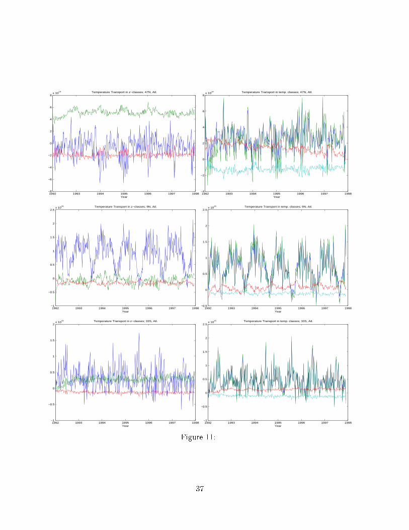
transport changes in our solution. In Fig. 11 is the split total heat transport there in Fig. 11

various contributions originating from di�erent parts of the water column. The �gure

shows temperature transport in various depth classes: (0-50m; 50-800, and below 800m),

Hq = �cp

�Z 0

�50v�dz +

Z�50

�800v�dz +

Z�800

�hv�dz

�: (6)

Also shown is the heat transport split into temperature classes: (� > 10ÆC; 4ÆC < � <

10ÆC; � < 4ÆC), so that,

Hq = �cp

Z 0

z(10o)v�dz +

Z z(10o)

z(4o)v�dz +

Z z(4o)

�hv�dz

!: (7)

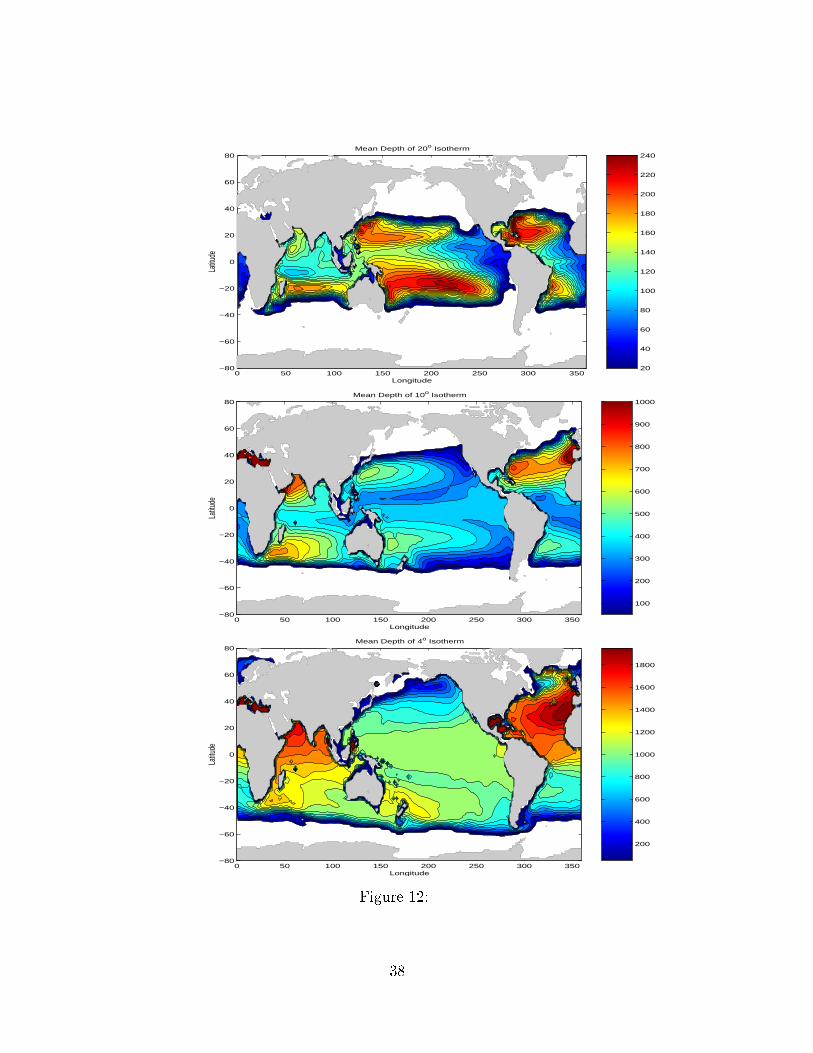
The mean depths of the 10ÆC and 4ÆC isotherms are given in Fig. 12 for the global Fig. 12

model domain together with a map of the 20Æ isotherm depth (compare Fig. 1). Gyre

signatures are conspicuous, as are the source regions for water masses and ventilation

\windows".

A summary of the overall result is that the largest part of the variability is associated

with the shallow near-surface layers that are dominated by high frequency near-surface

Ekman transports (compare Jayne and Marotzke, 2001). We note that the annual cy-

cle increases towards the equator and that the high-frequency variations in temperature

transports in the near-surface range are not compensated instantaneously by deeper com-

pensating transports at most latitudes. Only at 47ÆN can signi�cant compensation be

seen, and during winter months alone. As a result, most of the corresponding heat must

be stored locally and is then redistributed by the shallow layers. In contrast to the shallow

regions, the deeper layers show more seasonal to interannual variations. Nevertheless, the

shallow wind-driven variations also display interannual variations of amplitudes similar to

the deeper part, especially in high latitudes as shown here for the North Atlantic. Note

11

a clear upward trend in the temperature transport of the class � > 10Æ; while the next

lower � class decreases in its transport at 47ÆN indicating the warming of the deeper layers

there on basin average.

While our estimates do show drifts in deep temperatures, especially in the North

Atlantic and Southern Ocean, some of it may re ect actual ocean variability. Levitus

et al. (2000) and Barnett et al. (2001) discuss the temperature increase in the ocean

over the last decade as deduced from ocean data and from a coupled ocean-atmosphere

numerical climate simulation. Both analyses show signi�cant and comparable increases

in deep temperature in both the North Atlantic Southern Oceans. Separating numerical

drifts from climate related trends in the deep ocean will be a challenge for long-term

climate simulations and estimations.

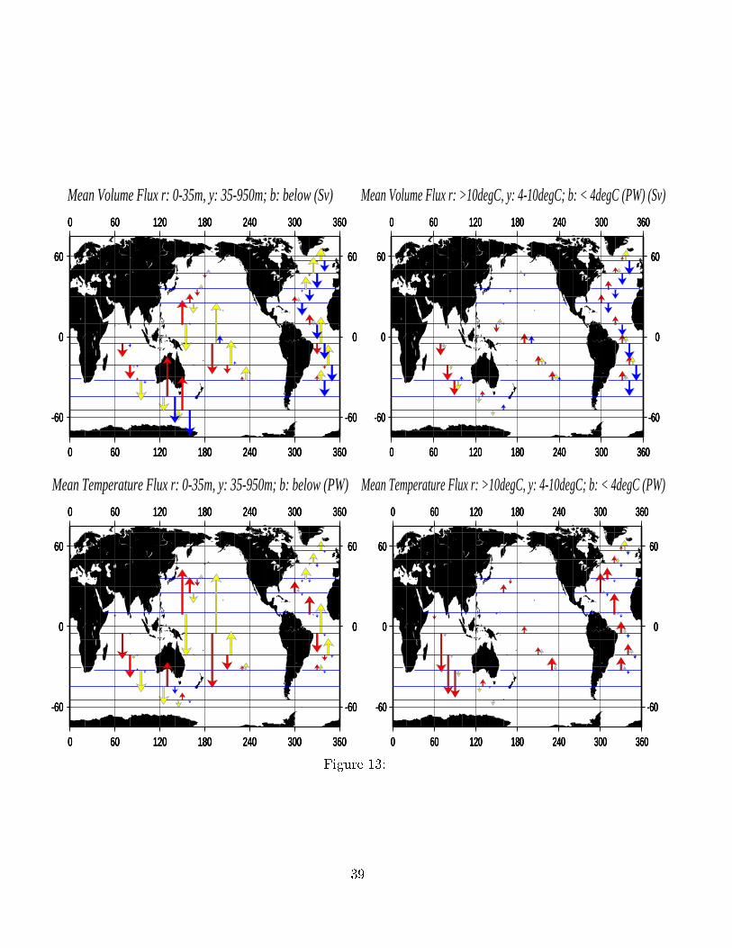
In Fig. 13 we show the time-mean volume and temperature transports analogous to Fig. 13

Fig. 3b, but now separated by depth and temperature classes. The shallow nature of

the Ekman cells is apparent|with high volume being transported in one direction near

the surface and returned in the next depth class. As a consequence of the shallow nature

of the cell, its e�ect is basically averaged out in the temperature classes. Water warmer

than 4ÆC moves northward in the Atlantic and colder water returns southward. Near the

equator and north of it, water warmer than 10ÆC carries the entire northward volume

ux.

Associated with the shallow overturning cell is a strong temperature transport, es-

pecially in the tropical oceans and over large regions of the Paci�c Ocean. Note that

most of the temperature transport variability occurs at temperatures above 10ÆC and

that the temperature transports in the two lower temperature classes nearly compensate

each other. In general terms, the Indian Ocean carries warm water southward, and which

subsequently is returned northward in the Atlantic via the \coldwater" route through

Drake Passage.

In the South Paci�c, a northward ow has contributions from all temperature classes,

but with the main component lying above 4ÆC. This water is returned southward in the

Indian Ocean|generally above 10ÆC. In the North Paci�c, each temperature class seems

to be balanced in terms of its volume ux, and no largescale net temperature ux is

apparent.

12

There also exists (not shown) a signi�cant seasonal cycle in the temperature ux

along the ACC south of the Cape of Good Hope with vigorous short-period variations

superimposed. Across Drake Passage, the transports are much more stable and vary

mostly in a small amplitude seasonal cycle. In contrast, south of Australia no visible

seasonal cycle appears, and temperature ux variations have much of the character of the

volume uxes (Fig. 4).

To investigate the various components present, we write the transport across each of

the sections in the form

Hq(t) =Z L

0

Z 0

�Hv�dzdx+

Z L

0

Z 0

�Hv0(t)�0(t)dzdx+

Z L

0

Z 0

�H�v0(t)dzdx+

Z L

0

Z 0

�Hv�0(t)dzdx

(8)

where integrals are being taken along zonal sections and where the bar indicates the time-

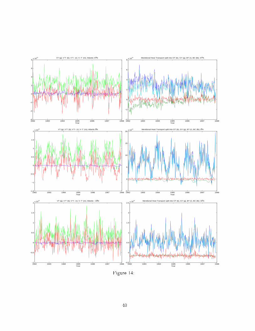
average. The decomposition is shown in Fig. 14 (except the �rst right-hand term). The Fig. 14

last term, in �0; gains importance towards high latitudes and is responsible for almost all

seasonal changes there. Note that both terms involving v0 tend to be of opposite sign at

mid- and high latitudes during all winter seasons (i.e. in winter time enhanced merid-

ional ow carries colder water), and are in phase during summer. Towards low latitudes,

most of the variability is in the v0T term, while the two other terms are very small. In

summary, accurate ow estimates are the most important information for estimating the

time-varying temperature transports in low latitudes, while at high latitudes both the

changing ow and temperature �elds must be known.

Another way to look at the temperature/heat uxes is to separate their contributions

to the vertical overturning from that of the horizontal gyre e�ect, or equivalently the

vertical mean contribution from the vertically varying one. To do so, de�ne ~V (z; t) as the

zonal average of V (x; z; t), ~V (x; z; t)0 = V (x; z; t)� ~V (z; t) and Vd as the vertical average

and V 0

d(x; z; t) = V (x; z; t) � Vd. Then the heat ux can be written as (see also B�oning

and Bryan, 1996)

Fq = �cp

Z L

0h(x)VdTddx+

Z L

0

Z 0

�h(x)V 0

dT0

ddzdx = F0 + F1; (9)

13

i.e., split into a depth independent, and depth-dependent components. (Note that purely

baroclinic ows produce non-zero vertical average volume uxes, and it would be incorrect

to call F0 the \barotropic" component.) h(x) is the water depth. Equivalently, we can

write,

Fq = �cp

Z L

0

Z 0

�h(x)

~V ~Tdzdx +Z L

0

Z 0

�h(x)

~V 0 ~T 0dzdx

!= FOT + FG; (10)

i.e., divided into overturning and gyre components. Further sub-decomposition is possible

and these decompositions are not unique.

Several surprising results are visible from the four Fj terms shown in Fig. 14 as zonal

integrals. High frequency changes in F0 and FOT are almost identical and dominate the

variability. As discussed in Jayne and Marotzke (2001), this variability arises from the

variable Ekman transport and a true barotropic return ow. At 47ÆN however, F0 and FOT

show di�erent secular trends. Although smaller in amplitude, F0 and FG are signi�cant,

with the latter slowly decreasing in amplitude over time except at high frequencies. Near

the equator, F0 becomes almost white noise, but FG shows an interesting seasonal cycle.

Further south, F0 becomes more signi�cant, with FG becoming very small.

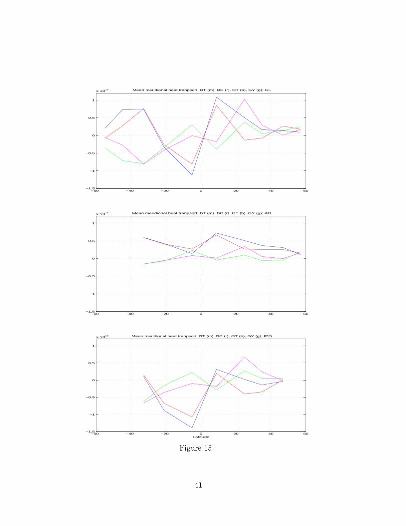
Fig. 15 shows time mean values of Fj as a function of latitude for the global ocean Fig. 15

and separately for the Atlantic and Indo-Paci�c sectors. Surprisingly, around 25ÆN, F0 is

the dominant transport mechanism on the global average. Towards higher latitudes, all

Fj become small, but equatorwards, F1 and FOT dominate. (The reader is reminded that

these are not additive contributions.)

In the Indo-Paci�c F0 is large in the northern hemisphere and south of the equator,

and largely compensated by F1 north of the equator. In the Atlantic, F1 or FOT dominate,

but around 25ÆN, F0 is enhanced, while FG grows south of the equator. A comparison with

Fig. 4.11 and 4.12 in B�oning and Bryan (1996) shows that our results are almost identical

to theirs in terms of the general structure, especially for the overturning component from

the 1/3Æ CME results. But our gyre component is somewhat smaller than their result

from a 1Æ model version of the North Atlantic. In agreement with the present results, the

CME shows an enhanced F0, although it is slightly further north, near 30ÆN. The basic

di�erence is that we obtain only a small fraction of their depth-independent amplitude|

14

with more than 1 PW carried there in the CME result.

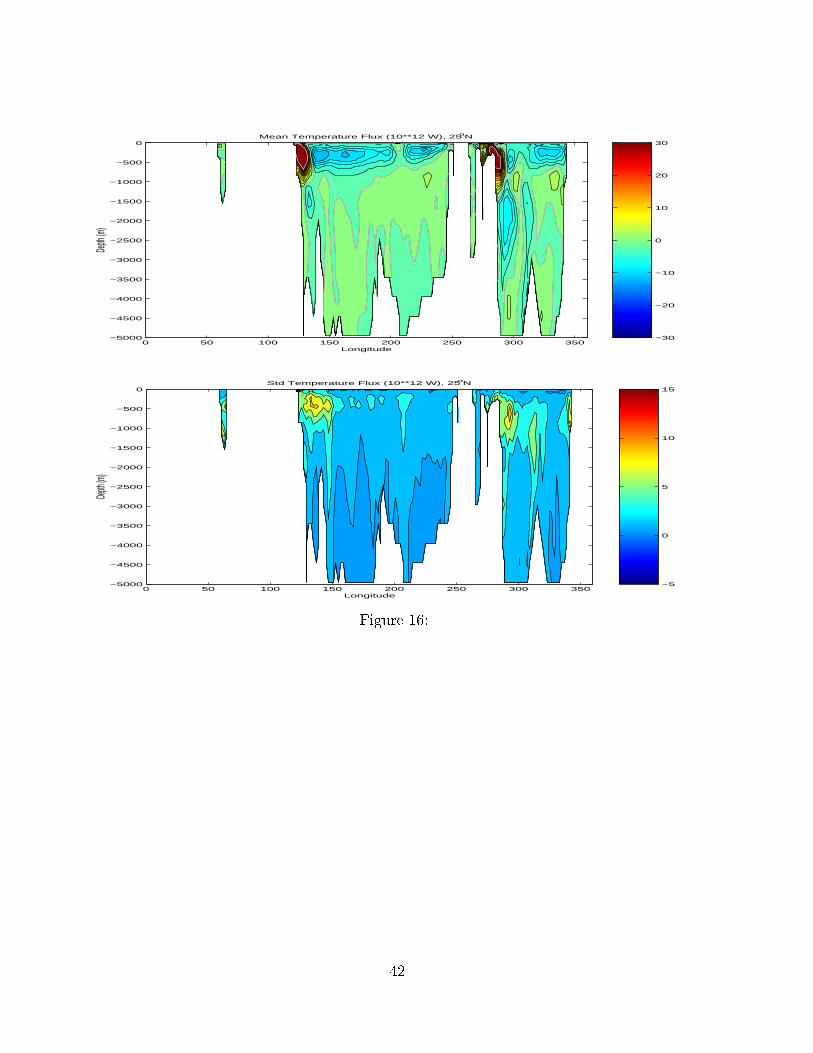
Fig. 16 displays zonal sections of the time-mean vT as a function of longitude and Fig. 16

depth. Note the similar structures of temperature transports in the Paci�c and Atlantic,

including the negative (southward) ux at the western boundary owing to similar, but

weaker and more shallow a deep western boundary current in the Paci�c Ocean. The stan-

dard deviation of vT is almost the same as that of v0T . Note the substantial uctuations in

mid-depth, especially near all western and eastern boundaries, but also over pronounced

topographic features. This variability originates from strong �rst mode Rossby waves,

some of which originate at the eastern boundary and propagate westward interacting

with the mid-ocean ridges (Herrmann and Krauss, 1989)

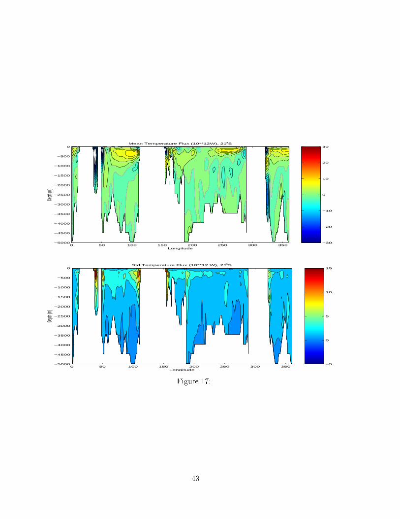
Fig.17 displays similar �elds, but for the Southern Hemisphere along 21ÆS. Note the Fig. 17

second-mode structures of the temperature transports and their variances in almost all

western and eastern boundary currents at this latitude. Highest variations in transports

are generally located at the transition in the mean transports from positive to negative.

Note also the large southward transports on both sides of Madagascar, which extends

over a large fraction of the entire water column.

5 Global and Regional Heat Balances

An important question concerns the way in which the ocean transports and stores heat

and how it communicates any regionally imbalanced heat ux through the surface to the

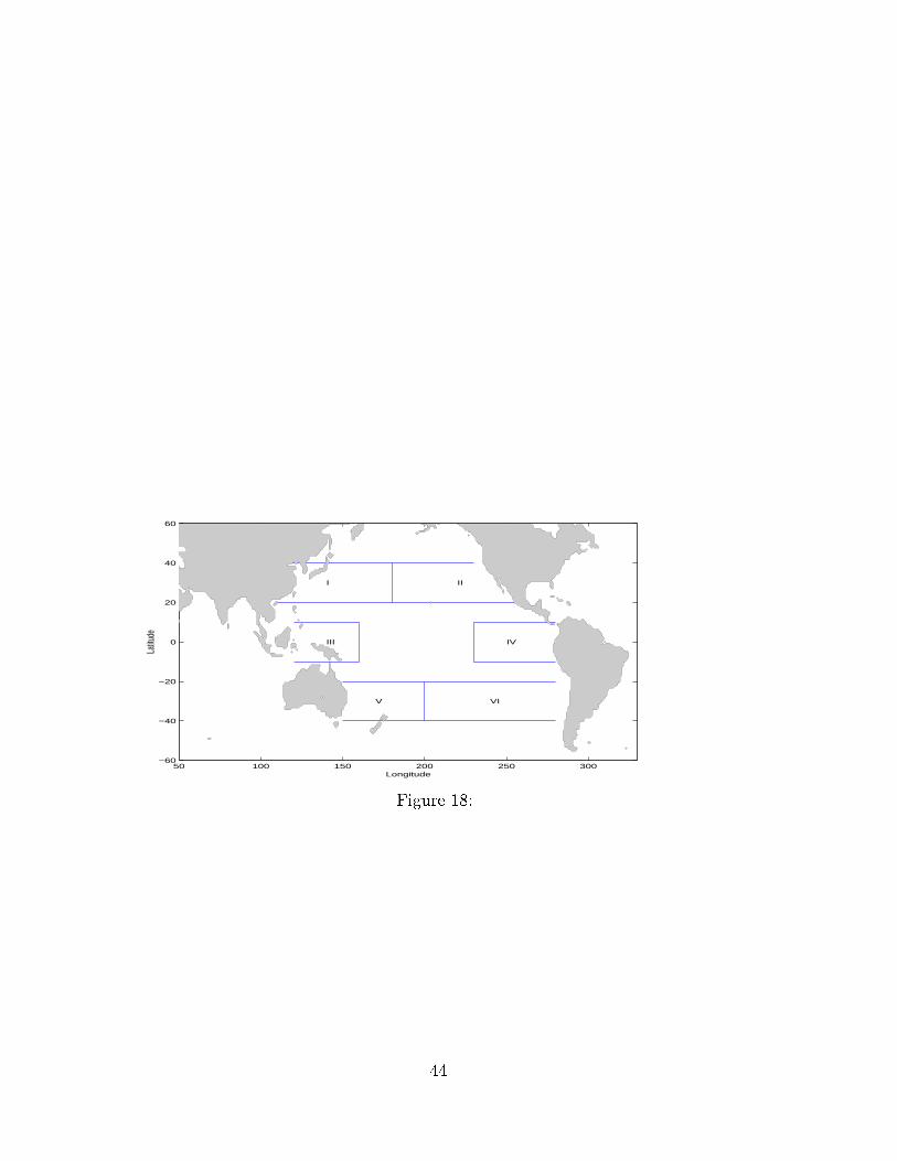
atmosphere. Consider the heat content changes in various regions of the Paci�c Ocean as

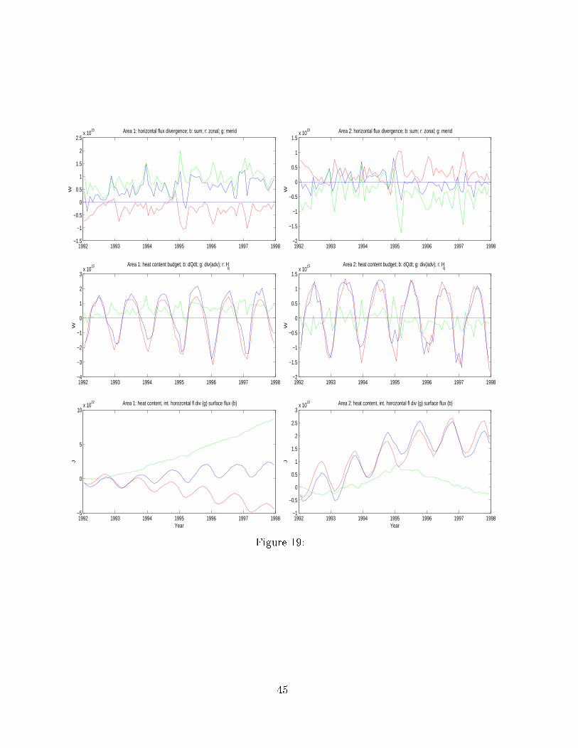
shown in Fig. 18 . Area 1 includes the Kuroshio Extension in the North Paci�c. Zonal Fig. 18

and meridional horizontal transport divergences as well as their net contribution to the

temperatures uxed into the region are displayed in the upper panel of Fig. 19. The net Fig. 19

lateral in ux is clearly positive, indicating that the region is being supplied by heat from

the ocean; in a steady state the excess must be released to the atmosphere.

In the middle panel of the same column, we show again the net horizontal temperature

ux divergence, together with the net surface heat ux of the same region and the net

oceanic heat content change dQ=dt. The net oceanic heat in ux is balanced by a net

15

surface heat ux over that region of -8.8 W/m2 leading to a almost stable heat content

that varies only on the seasonal cycle (bottom panel).

Further to the east (Region II) the situation is somewhat di�erent. Here the heat

content is steadily rising over the six-year integration period. It was shown in Fig. 2 that

XBT observations are consistent with this heat content increase (compare also Barnett et

al., 2001). Convergence of the horizontal uxes is positive zonally and negative meridion-

ally. The net e�ect is slightly positive over the �rst part of the period, but turns negative

subsequently, i.e., the ocean then carries heat out of this region. Net surface heat ux is

also positive (6.6 W/m2) and the heat content increase here can now be identi�ed as a

joint e�ect of horizontal transport convergence and surface ux during the �rst few years.

The transport divergence subsequently halts and reverses the trend in the heat content.

This is a good example showing that, although small in amplitude, oceanic transports

and convergences, accumulate over long periods to produce substantial e�ects.

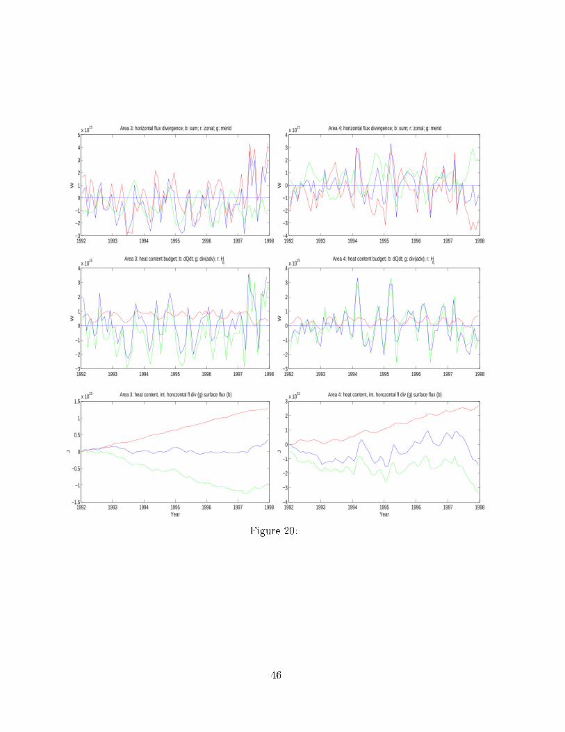
Region III and IV are located at the western and eastern side of the tropical Paci�c,

respectively (Fig. 20). Horizontal ux convergences are large here and show signs of Fig. 20

ENSO e�ects, especially at the western side at the end of the period when the zonal

convergence is markedly positive. At the eastern side, the zonal convergence is negative

during 1997, but the meridional convergence becomes positive at almost the same rate,

giving rise to only a small net negative transport convergence here. Note that in both

regions, temporal changes in the oceanic heat content are dominated by the horizontal

advection of temperature in and out of the regions.

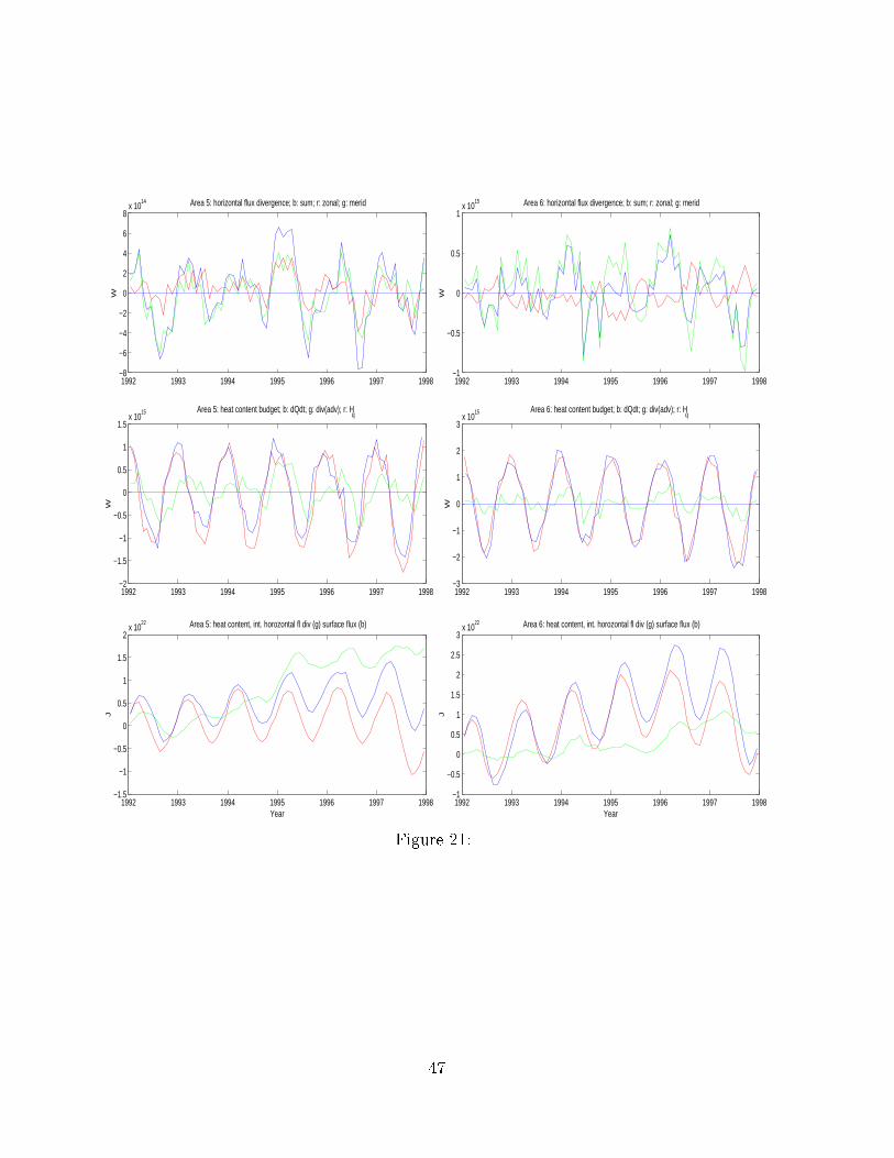
Region V covers the area of the East Australia current (Fig. 21). There, the ocean ow Fig. 21

changes markedly with the seasonal cycle. Boreal winters lead to net in ow of temperature

and the ux is reversed six months later. The changes in the oceans net heat contents are

somewhat smaller than the net surface heat ux �elds would suggest and heat content

variations on seasonal and interannual timescale are dominated by variations in horizontal

ux divergences.

Finally, Region VI is located at the eastern side of the subtropical South Paci�c. Note

that the southern edge is in uenced by enhanced high frequency wind-driven barotropic

variability as documented, e.g., by Fukumori at el. (1998) and Stammer et al. (2000)

16

(compare also Fig. 6). Meridional transport convergences are accordingly quite vigorous

at high-frequencies, but to some extent are balanced by the zonal convergences and net

e�ects are smaller than were seen on the western side. So again, the surface heat ux

dominates the variability of net oceanic heat content changes, although longer-period

variations due to changing ocean currents do exist.

6 Summary and Conclusions

A dynamically consistent time-dependent combination of a GCM and global data has

been used to estimate ocean transports of volume, heat and fresh water and to analyse

their temporal changes. Emphasis was put especially on an estimate of global oceanic

cycles of heat storage and heat ux quantities of signi�cant climate relevance. Because

the quality of the underlying ow estimates is limited by the present low resolution, the

most important results here are the demonstration that these computations are feasible.

The estimates will gradually improve through the addition of new data, more complete

model physics and higher resolution, but the present solution is probably among the best

that can be done today. In particular, the analysis of the temporal variability of the ux

properties is believed to be accurate except for the variability owing to the unresolved

eddy �eld.

An important result from this study is that time-average uxes estimated from this

fully time-dependent circulation have converged with independent steady- ow estimates

from box inversions over most parts of the world ocean but especially in the southern

hemisphere. This was previously not the case; instead full assimilation attempts based

on GCMs usually di�ered signi�cantly from those based on simpli�ed box inversions with

more con�dence being put into the latter as has been discussed in detail by Marotzke and

Willebrand (1996). However, transport estimates still di�er substantially in the North

Atlantic where our estimates result in only 1/2 previous heat transports.

Although the low model resolution causes problems with estimates of the time average

proprty uxes, the patterns in the means are in encouraging quantitative agreement with

the independent estimates of Ganachaud and Wunsch (2000). Equally important, we ob-

17

tain an estimate of the ocean state that is basically in balance with simultaneous estimates

of surface uxes of momentum, heat and freshwater ux. The meridional heat transports

estimated from both transports within the model and from integrals of the surface heat

uxes are mostly consistent with the exception of the North Atlantic and within error

bars of Trenberth et al. (2001), in a comparison of NCEP, ECMWF, and COADS-derived

values. A more complete discussion is provided in Stammer et al. (2001b).

Mean and time-varying volume uxes for the entire three dimensional ocean circulation

are estimated. Among the more striking results are the con�rmation of previous �ndings

of a mean circulation around Australia which involves a net volume ux of 14 Sv through

the Indonesian Through ow and the Mozambique Channel. In addition, we show that

this ow regime exist on all time scales longer than one month rendering the variability

in the South Paci�c strongly coupled to the Indian Ocean. Accordingly, the ACC shows

a superposition of those regional ow changes to the global transports around Antarctica

that are dominated by a seasonal cycle. An estimated mean ACC transport of 138 Sv is

in good agreement with previous observational �ndings.

The temporal variability of oceanic heat ux, heat storage and atmospheric exchanges

is complex, showing a dependence upon location, depth, and time-scale as described

above. Oceanic transports, storage, and air/sea exchange follow a complicated geographi-

cal pattern and exhibit variability on all accessible time scales. For the �rst time, we now

have a prototype ocean data synthesis tool that provides a quantitative ocean transport

analysis.

The description given here of the oceanic heat budget remains tentative owing to

remaining model/data shortcomings already described. However, we anticipate rapid

improvement in all of the elements of the budget through model and data improvements

now underway. Ongoing computations will complete a WOCE data synthesis including,

in addition to the data used here, the WOCE hydrography, global XBT data sets,

TOA temperature measurements, drifter surface velocities, etc. Computations are being

carried out now on a nominal 1 Æ grid and include mixed layer dynamics. These and

related computations will likely be the pattern for future design and synthesis of all

future large-scale observation programs.

18

Acknowledgments. Computational support from the National Partnership for

Computational Infrastructure (NPACI) and the National Center for Atmospheric Re-

search (NCAR) is acknowledged. Supported in part through ONR (NOPP) ECCO grants

N00014-99-1-1049 and N00014-99-1-1050, through NASA grant NAG5-7857, through NSF

grant OCE 9730071 and through two contracts with the Jet Propulsion Laboratory

(958125 and 1205624).

References

[1] Barnett, T., D.W. Pierce and R. Schnur, 2001: Detection of anthropogenic climate

change in the world's ocean. Science, 292, 270{274.

[2] C. F. Bohren and B. A. Albrecht, Atmospheric Thermodynamics, Oxford Un. Press,

New York, 1998, 402 pp.

[3] B�oning, C.W., and F.O. Bryan, 1996: Large-scale transport processes in high-

resolution circulation models. In: The Warmwassersphere of the North Atlantic. W.

Krauss (ed.), Gebr. Borntr�ager, Stuttgart, pp. 91-128.

[4] Carton, J.A., G. Chepurin, X. Cao, and B.S. Giese, 2000a: A Simple Ocean Data

Assimilation analysis of the global upper ocean 1950-1995, Part 1: methodology, J.

Phys. Oceanogr., 30, 294-309.

[5] Carton, J.A., G. Chepurin, and X. Cao, 2000b: A Simple Ocean Data Assimilation

analysis of the global upper ocean 1950-1995 Part 2: results, J. Phys. Oceanogr., 30,

311-326.

[6] Fukumori, I., R. Raghunath, and L.-L. Fu, 1998: Nature of global large-scale sea

level variability in relation to atmospheric forcing: a modeling study, J. Geophys.

Res., 103, 5493-5512.

19

[7] Ganachaud, A. and C. Wunsch, 2000: Oceanic meridional overturning circulation,

mixing, bottom water formation rates and heat transport. Nature, 408, 453-456.

[8] Garnier, E., B. Barnier, L. Siefridt and K. B�eranger, 2001: Investigating the 15 years

air-sea ux climatology from the ECMWF reanalysis project as a surface bound-

ary condition for ocean models. International Journal of Climatology, submitted for

publications.

[9] Gordon, A.L., 1986: Interocean exchange of thermocline water. J. Geophys. Res., 91,

5037{5046.

[10] Godfrey, J.S., 1996: The e�ect of the Indonesian through ow on ocean circulation

and heat exchange with the atmosphere: A review. J. geophys. Res., 101, 12,217{

12,2238.

[11] Herrmann, P. and W. Krauss, 1998: Generation and propagation of annual Rossby

waves in the North Atlantic. J. Phys. Oceanogr., 19, 727{744.

[12] Jayne, S.R. and J. Marotzke, 2001: The dynamics of ocean heat transport variability.

Rev. Geophys., 39, 385{412.

[13] Josey, S.A., E.C. Kent and P.K. Taylor, 1999: New insight into the ocean heat

budget closure problem from analysis of the SOC air-sea ux climatology. J. Clim.,

12, 2856{2880.

[14] Lemoine, F. and 17 others The development of the NASA GSFC and NIMA Joint

Geopotential Model. in, Proceedings of the International Symposium on Gravity,

Geoid and Marine Geodesy, IAG Symposium: in press H. Fujimoto, ed. Springer-

Verlag.

[15] Levitus, S., J.I. Antonov, J. Wang, T.L. Delworth, K.W. Dixon and A.J. Broccoli,

2000: Anthropogenic warming of Earth's climate system. Science, ???.

20

[16] Levitus, S., R. Burgett, and T. Boyer, World Ocean Atlas 1994, vol. 3, Salinity, and

Vol. 4, Temperature, NOAA Atlas NESDIS 3 & 4, U.S. Dep. of Comm., Washington,

D.C., 1994.

[17] Macdonald, A.M., The global ocean circulation: a hydrographic estimate and regional

analysis. Prog. Oceanography, 41, 281{382, 1998.

[18] Macdonald, A.M., and C. Wunsch, An estimate of global ocean circulation and heat

uxes, Nature, 382, 436-439, 1996.

[19] Marotzke, J., J. Willebrand, 1996: The North Atlantic mean circulation: combining

data and dynamics. In Warm Water Sphere of the North Atlantic Ocean, edited by

W. Krauss, Gebr�uder Borntr�ager, Berlin, 159{193.

[20] Marshall, J., A. Adcroft, C. Hill, L. Perelman, and C. Heisey, A �nite-volume,

incompressible navier-stokes model for studies of the ocean on parallel computers. J.

Geophys. Res. , 5753{5766, 1997.

[21] McPhaden MJ, Busalacchi AJ, Cheney R, Donguy JR, Gage KS, Halpern D, Ji

M, Julian P, Meyers G, Mitchum GT, Niiler PP, Picaut J, Reynolds RW, Smith N,

Takeuchi K, 1998: The tropical ocean global atmosphere observing system: A decade

of progress. J. of Geophys. Res., 103, 14169-14240.

[22] Nerem, R.S., D.P. Chambers, E.W. Leuliette, G.T. Mitchum, B.S. Giese, 1999: Vari-

ations in global mean sea level associated with the 1997-1998 ENSO event: Implica-

tions for measuring long term sea level change Geophys. Res. Lett., 26, 3005-3008.

[23] Nowlin, Jr., W.D., and J.M. Klink, 1986: The physics of the Antarctic Circumpolar

Current. Rev. Geophys. Space Phys., 24, 469{491.

[24] Ponte, R., D. Stammer and C. Wunsch, 2001: Improved ocean angular momentum

estimates using an ocean model constrained by large-scale data, Geoph. Res. Letters,

in press.

21

[25] Rintoul, S., 1991 South Atlantic inter-basin exchange. J. Geophys. Res., 96, 2675-

2692.

[26] Roach, A.T, K. Aagaard, C.H. Pease, S.A. Salo, T. Weingartner, V. Pavlov, and M.

Kulakov, 1995: Direct measurements of transport and water properties through the

Bering Strait, J. Geophys. Res., 100, 18,443-18,457.

[27] Roemmich, D., S. Hautala and D. Rudnick, 1996: Northward abyssal transport

through Samoan Passage and adjacent regions. J. Geophys. res., 101, 14039{14055.

[28] Stammer, D., C. Wunsch, and R. Ponte, 2000: De-aliasing of global high frequency

barotropic motions in altimeter observations, Geophysical Res. Letters, 27, 1175-1178.

[29] Stammer, D., C. Wunsch, R. Giering, C. Eckert, P. Heimbach, J. Marotzke, A.

Adcroft, C.N. Hill, and J. Marshall, 2001, The global ocean circulation during 1992

{1997, estimated from ocean observations and a general circulation model, submitted

for publication.

[30] Stammer, D., K. Ueyoshi, W. Large and C. Wunsch, 2001b: Surface Fluxes Estimated

Through Ocean Data Assimilation, to be submitted.

[31] Tierney, C., J. Wahr, F. Bryan and V. Zlotnicki, 2000: Short-period oceanic circula-

tion: implications for satellite altimetry. Geophys. res. Letters, 27, 1255{1258.

[32] Trenberth,.K. E., J. M. Caron and D. P. Sepaniak. The atmospheric energy budget

and implications for surfaces uxes and ocean heat transports. Clim. Dyn., 17, 259-

276, 2001.

[33] Warren, B. A. Approximating the energy transport across oceanic sections J. Geophys

Res., 104, 7915-7919, 1999.

[34] Whitworth, T, Monitoring the transport of the Antarctic Circumpolar Current at

Drake Passage. J. Geophys. Res., 13, 2045-2057, 1983.

[35] Wij�els, S.E., R.W. Schmitt, H. Bryden and A. Stigebrand, 1992: Transport of

freshwater by the ocean. J. Phys. Oceanogr., 22, 155-162.

22

Figure Captions

Fig. 1: (top) Depth of 20Æ isotherm as a function of time evaluated from TOGA TAO

data from 140Æ to 150Æ E on the equator (blue dots). Red and green dots are estimates

at the same location obtained from the unconstrained and constrained model runs,

respectively. (middle) Same as top panel, but from 265Æ E on the equator. (bottom)

Zonal di�erence in the depth of the 20Æ isotherm, evaluated from the unconstrained

(blue) and constrained model (red), respectively.

Fig. 2: Heat content (Joules) estimated over 20Æx20Æ regions centered at 190ÆE, 30ÆN

and 150ÆE, 10ÆS. Red lines are the results from the unconstrained model. Blue lines

show results from XBTs, and the green lines are results from the constrained model.

Fig. 3: (top) Mean and standard deviations of volume ux (Sv) across sections as

shown. (bottom) Mean and standard deviations of temperature transports (converted to

Petawatts, PW) across various sections .

Fig. 4: Top panel: Time series of volume transports from the South Paci�c across 36ÆS

(green); along the ACC south of Australia (red) with the large-scale ACC component

through Drake Passage removed. Negative values are from the the Indonesian

Through ow (blue curve) and the Indian Ocean across 36ÆS (magenta). Right inset

shows a short segment of the high-pass �ltered timeseries in the Paci�c Ocean (blue) and

across the Madagascar Channel (red, with opposite sign). Middle panel: Time series of

the Mozambique Channel Through ow minus that through the Indonesian Through ow

(red curve) and the transport going north across the remaining Indian Ocean at 20ÆS

(blue curve). Bottom panel: The ACC transports south of Africa, Australia, and and

through Drake Passage shown as blue, green and red curves, respectively.

Fig. 5: (a) Power spectral density of volume ux time series from 21ÆS across the South

Paci�c (solid curve) and across the Mozambique Channel minus the Indian Ocean at

23

that location (dashed curve). (b) Coherence amplitude for the two timeseries shown in

(a). (c) Coherence phase for the two time series with the sign of the Madagascar

Channel transport reversed for display purposes.

Fig. 6: log10 of the standard deviation of meridional velocity v as a function of depth

and longitude along 31ÆS across the Paci�c and Indian Ocean.

Fig. 7: (top) Mean sea surface height changes over the six year simulation period

estimated from a least-squares �t procedure. Contour interval is 5 cm. (bottom)

Time-mean meridional volume transports (SV) integrated zonally acoss the entire model

domain.

Fig. 8: Top panel: Integrated time-mean meridional heat transports for the global

ocean estimated for various zonal sections in the model (blue curve). The blue error

bars are estimated as �=pN where � is the standard deviation in time of those uxes,

evaluated over the 5 year period every 5 days and N = 435, assuming individual

estimates are independent. The green error bars mark the standard deviation obtained

from individual annual mean estimates. The red curve represents the ocean heat

transport inferred from estimated surface heat uxes. Middle and bottom panels:

Estimated meridional heat transport across zonal section sin the model, evaluated

separately for the Atlantic, Paci�c-Indian Oceans. All red symbols represent estimates

from Ganachaud and Wunsch (2000) at the respective latitudes and their formal

uncertainties.

Fig. 9: Top panel: Integrated time-mean meridional fresh water transports (in kg/s) for

the global ocean estimated from zonal sections in the model. Blue error bars are

estimated similar to those for heat uxes. The green error bars mark the standard

deviation obtained from individual annual mean estimates. Red symbols represent

estimates from Wij�els et al (1992) at the respective latitudes. Middle and bottom

panels: Estimated meridional fresh water transport across zonal section in the model,

24

evaluated separately for the Atlantic, Paci�c-Indian Oceans.

Fig. 10: Zonally integrated heat (top in W) and and surface fresh water uxes (bottom

in Kg/s), evaluated globally (blue curves) and over the Atlantic (red), Paci�c (green)

and Indian Ocean (magenta) sectors, respectively.

Fig. 11: Timeseries of temperature transports across several latitude circles in the

Atlantic as indicated in the panels. The left column shows those transports evaluated

over the depth classes (0-50m) (blue), (50-800m) (green) and (800 - bottom) (red). The

right column similar transports are shown but evaluated over temperature classes

(>10ÆC) (green), (10ÆC > � > 4ÆC) (red) and (< 4ÆC) (light blue). The blue curve

shows the total temperature transport.

Fig. 12: (top) Mean depths of (top) the 20ÆC isotherm, (middle) the 10ÆC isotherm and

(bottom) the 4ÆC Isotherm. In meters.

Fig. 13: Maps of the mean volume (top) and temperature (bottom) transports. The

left column shows results for depth classes, while the right column shows similar results

for temperature classes.

Fig. 14: (left) Timeseries HQ(t) =R R

v�dzdx (green curves) across zonal sections with

locations given in the panels. Also shown areR R

v0�0dzdx,R R

�v0dzdx andR R

v�0dzdx

as blue, red and magenta lines, respectively. (right) Temperature transport time series

evaluated as contributions from the overturning (OT; blue), the gyre (GY; green), the

barotropic (BT, red) and baroclininc circulation (BC, light blue), respectively. See text

for details.

Fig. 15: (a) Zonally integrated heat transports resulting from the overturning (OT;

blue), the gyre (GY; green), the barotropic (BT, magenta) and baroclininc circulation

(BC, red), respectively. The middle and lower panels show similar results but separately

25

for the Atlantic and Indian-Paci�c sectors.

Fig. 16: Zonal sections of the time-mean vT as a function of longitude and depth along

25ÆN. The lower two panels show the standard deviation of vT which is almost the same

as v0T .

Fig. 17: Zonal sections of the time-mean vT as a function of longitude and depth along

21ÆS. The lower two panels show the standard deviation of vT which is almost the same

as v0T .

Fig. 18: Map showing regions 1 - 6 for which the heat content budget is shown in Figs.

19 - 21.

Fig. 19: (top) Horizontal temperature ux divergence in area 1 (left) and area 2 (right),

plotted separately for the zonal contributions (red), the meridional contributions (green)

and the net convergence (blue). (middle) Horizontal temperature ux convergence

(green), net surface heat ux (red) and time-rate of change of heat content in the area

(blue). (bottom) Timeseries of heat content (blue), integrated surface heat ux (red)

and integrated horizontal convergence (green).

Fig. 20: Same as in Fig. 19, but for areas 3 and 4.

Fig. 21: Same as in Fig. 19, but for areas 5 and 6.

26

1992 1993 1994 1995 1996 1997 1998100

150

200

250

Year

Depth of 20o Isotherm, 140o−150oE

1992 1993 1994 1995 1996 1997 19980

50

100

150

Year

Depth of 20o Isotherm, 265oE

1992 1993 1994 1995 1996 1997 1998−160

−140

−120

−100

−80

−60

−40

Year

Zonal Difference of 20o Isotherm Depth

Figure 1:

27

1992 1993 1994 1995 1996 1997 19982.9

3

3.1

3.2

3.3

3.4

3.5

3.6

3.7

3.8

3.9x 10

10

Year

190o E, 30o N

1992 1993 1994 1995 1996 1997 19982.8

2.9

3

3.1

3.2

3.3

3.4

3.5x 10

10

Year

150o E, 10o S

Figure 2:

28

-60

0

60

-60

0

60

0 60 120 180 240 300 360

0 60 120 180 240 300 360

0 ± 0.5 0 ± 1

0 ± 0.7 0 ± 1

0 ± 1 0 ± 1

0 ± 1.2 0 ± 1.3 0 ± 1.3

0 ± 2.4 13.3 ± 4 0 ± 1.5❘ ➞

6.5 ± 6 14.3 ± 4 0 ± 1.6❘ ➞➞❘

➞

-20.8 ± 5 -14.3 ± 4 14.3 ± 4 0 ± 1.9❘ ➞❘

➞

138 ± 8

❘ ➞151 ± 7

❘ ➞136 ± 7❘

➞

➞14.3 ± 5

Mean and SD Estimated Volume Flux (Sv)

-60

0

60

-60

0

60

0 60 120 180 240 300 360

0 60 120 180 240 300 360

➞-.01 ± .15 .28 ± .14

0 ± .39 .38 ± .26

➞.39 ± .62 .66 ± .31

➞ ➞-.1 ± .39 .41 ± 1.8 .26 ± .4

➞ ➞-.38 ± 1.3 .13 ± 1.3 .35 ± .38

-.26 ± .55 .24 ± .57 .32 ± .26➞ ➞➞

-1.02 ± .3 -1.02 ± .35 .52 ± .47 .38 ± .29❘ ➞❘

➞

1.02 ± .16

❘ ➞1.91 ± .12

❘ ➞1.25 ± .06❘

➞

➞1.34 ± .53

Mean and SD Estimated Temperature Flux (PW)

Figure 3:

29

1992 1993 1994 1995 1996 1997 1998−30

−20

−10

0

10

20

30

Year

Volum

e Fl

ux (S

v)

Volume Flux SP (b), IO (g), Indo (r), ACC (m)

1994 1995−10

−5

0

5

10

Year

HP filtered Volume Flux: b: SP; r: −IO

1992 1993 1994 1995 1996 1997 1998−25

−20

−15

−10

−5

0

5

10

15

20

25

Year

Volum

e Fl

ux (S

v)

Volume Flux Mada−Indo (r); IO(20S) (b)

1992 1993 1994 1995 1996 1997 1998100

110

120

130

140

150

160

170

Year

Volum

e Fl

ux (S

v)

Volume Flux Afr. (b), Austr. (g), Drake (r)

Figure 4:

30

10−3

10−2

10−1

1011

1012

1013

1014

1015

Frequency (CPD)

PSD Transports Ps (solid), Mada (dashed)

10−3

10−2

10−1

0

0.1

0.2

0.3

0.4

0.5

0.6

0.7

0.8

0.9

1

Frequency (CPD)

Coherence Amplitude (P1,Mada)

10−3

10−2

10−1

−80

−60

−40

−20

0

20

40

60

80

Frequency (CPD)

Coherence Phase (P1,Mada)

Figure 5:

31

−3.2

−3

−2.8

−2.6

−2.4

−2.2

−2

−1.8

50 100 150 200 250−4500

−4000

−3500

−3000

−2500

−2000

−1500

−1000

−500

0

Longitude

log−10(rms(v))

Figure 6:

32

−40

−30

−20

−10

0

10

20

30

40

0 50 100 150 200 250 300 350−80

−60

−40

−20

0

20

40

60

80

Longitude

Latitu

de

SSH drift over 6 yrs (cm)

1

−80 −60 −40 −20 0 20 40 60 80−0.5

0

0.5

1

1.5

2

2.5

3

3.5

4x 10

−3

Latitude

Mean global meridional Volume Flux (m3/s)

Figure 7:

33

−60 −40 −20 0 20 40 60−2

−1.5

−1

−0.5

0

0.5

1

1.5

2x 10

15

Latitude

Northward Heat Transport (o=GW; W/m2)

−60 −40 −20 0 20 40 600

2

4

6

8

10

12

14

16x 10

14

Latitude

Northward Heat Transport, Atlantic (o=GW; W/m2)

−60 −40 −20 0 20 40 60−2.5

−2

−1.5

−1

−0.5

0

0.5

1x 10

15

Latitude

Northward Heat Transport, Indo−Pacific (o=GW; W/m2)

Figure 8:

34

−60 −40 −20 0 20 40 60−1

−0.8

−0.6

−0.4

−0.2

0

0.2

0.4

0.6

0.8

1x 10

9

Latitude

Northward Fresh Water Transport (o=WI; W/m2)

−40 −30 −20 −10 0 10 20 30 40 50−4

−3

−2

−1

0

1

2x 10

8

Latitude

Mean net Freshwater Transport, Atlantic

−60 −40 −20 0 20 40 60−8

−6

−4

−2

0

2

4

6

8x 10

8 Northward Freshwater Transport, Indo−Pacific (o=GW; W/m2)

Latitude

Figure 9:

35

−80 −60 −40 −20 0 20 40 60 80−1

−0.5

0

0.5

1

1.5

2

2.5

3

3.5

4x 10

14

Latitude

Net surface heat flux (W)

−80 −60 −40 −20 0 20 40 60 80−2

−1.5

−1

−0.5

0

0.5

1

1.5

2x 10

8

Latitude

Net surface freshwater flux (kg/s)

Figure 10:

36

1992 1993 1994 1995 1996 1997 1998−8

−6

−4

−2

0

2

4

6

8x 10

14

Year

Temperature Transport in z−classes; 47N, Atl.

1992 1993 1994 1995 1996 1997 1998−4

−2

0

2

4

6

8x 10

14

Year

Temperature Transport in temp. classes; 47N, Atl.

1992 1993 1994 1995 1996 1997 1998−1

−0.5

0

0.5

1

1.5

2

2.5x 10

15

Year

Temperature Transport in z−classes; 9N, Atl.

1992 1993 1994 1995 1996 1997 1998−0.5

0

0.5

1

1.5

2

2.5x 10

15

Year

Temperature Transport in temp. classes; 9N, Atl.

1992 1993 1994 1995 1996 1997 1998−1

−0.5

0

0.5

1

1.5

2x 10

15

Year

Temperature Transport in z−classes; 33S, Atl.

1992 1993 1994 1995 1996 1997 1998−1

−0.5

0

0.5

1

1.5

2

2.5x 10

15

Year

Temperature Transport in temp. classes; 33S, Atl.

Figure 11:

37

20

40

60

80

100

120

140

160

180

200

220

240

0 50 100 150 200 250 300 350−80

−60

−40

−20

0

20

40

60

80

Longitude

Latitu

de

Mean Depth of 20o Isotherm

100

200

300

400

500

600

700

800

900

1000

0 50 100 150 200 250 300 350−80

−60

−40

−20

0

20

40

60

80

Longitude

Latitu

de

Mean Depth of 10o Isotherm

200

400

600

800

1000

1200

1400

1600

1800

0 50 100 150 200 250 300 350−80

−60

−40

−20

0

20

40

60

80

Longitude

Latitu

de

Mean Depth of 4o Isotherm

Figure 12:

38

-60

0

60

-60

0

60

0 60 120 180 240 300 360

0 60 120 180 240 300 360

-60

0

60

-60

0

60

0 60 120 180 240 300 360

0 60 120 180 240 300 360

-60

0

60

-60

0

60

0 60 120 180 240 300 360

0 60 120 180 240 300 360

-60

0

60

-60

0

60

0 60 120 180 240 300 360

0 60 120 180 240 300 360

Mean Volume Flux r: 0-35m, y: 35-950m; b: below (Sv)

-60

0

60

-60

0

60

0 60 120 180 240 300 360

0 60 120 180 240 300 360

-60

0

60

-60

0

60

0 60 120 180 240 300 360

0 60 120 180 240 300 360

-60

0

60

-60

0

60

0 60 120 180 240 300 360

0 60 120 180 240 300 360

-60

0

60

-60

0

60

0 60 120 180 240 300 360

0 60 120 180 240 300 360

Mean Volume Flux r: >10degC, y: 4-10degC; b: < 4degC (PW) (Sv)

-60

0

60

-60

0

60

0 60 120 180 240 300 360

0 60 120 180 240 300 360

-60

0

60

-60

0

60

0 60 120 180 240 300 360

0 60 120 180 240 300 360

-60

0

60

-60

0

60

0 60 120 180 240 300 360

0 60 120 180 240 300 360

-60

0

60

-60

0

60

0 60 120 180 240 300 360

0 60 120 180 240 300 360

Mean Temperature Flux r: 0-35m, y: 35-950m; b: below (PW)

-60

0

60

-60

0

60

0 60 120 180 240 300 360

0 60 120 180 240 300 360

-60

0

60

-60

0

60

0 60 120 180 240 300 360

0 60 120 180 240 300 360

-60

0

60

-60

0

60

0 60 120 180 240 300 360

0 60 120 180 240 300 360

-60

0

60

-60

0

60

0 60 120 180 240 300 360

0 60 120 180 240 300 360

Mean Temperature Flux r: >10degC, y: 4-10degC; b: < 4degC (PW)

Figure 13:

39

1992 1993 1994 1995 1996 1997 1998−6

−4

−2

0

2

4

6

8x 10

14

Year

VT (g); V‘T‘ (b); V‘T− (r); V−T‘ (m); Atlantic 47oN

1992 1993 1994 1995 1996 1997 1998−4

−2

0

2

4

6

8x 10

14

Year

Meridional Heat Transport split into OT (b), GY (g), BT (r), BC (lb); 47oN

1992 1993 1994 1995 1996 1997 1998−1.5

−1

−0.5

0

0.5

1

1.5

2x 10

15 VT (g); V‘T‘ (b); V‘T− (r); V−T‘ (m); Atlantic 9oN

Year1992 1993 1994 1995 1996 1997 1998

−5

0

5

10

15

20x 10

14

Year

Meridional Heat Transport split into OT (b), GY (g), BT (r), BC (lb); 9oN

1992 1993 1994 1995 1996 1997 1998−1

−0.5

0

0.5

1

1.5

2x 10

15

Year

VT (g); V‘T‘ (b); V‘T− (r); V−T‘ (m); Atlantic −33oN

1992 1993 1994 1995 1996 1997 1998−0.5

0

0.5

1

1.5

2

2.5x 10

15

Year

Meridional Heat Transport split into OT (b), GY (g), BT (r), BC (lb); 33oS

Figure 14:

40

−60 −40 −20 0 20 40 60−1.5

−1

−0.5

0

0.5

1

x 1015 Mean meridional heat tranpsort; BT (m), BC (r), OT (b), GY (g); GL

−60 −40 −20 0 20 40 60−1.5

−1

−0.5

0

0.5

1

x 1015 Mean meridional heat tranpsort; BT (m), BC (r), OT (b), GY (g); AO

−60 −40 −20 0 20 40 60−1.5

−1

−0.5

0

0.5

1

x 1015

Latitude

Mean meridional heat tranpsort; BT (m), BC (r), OT (b), GY (g); IPO

Figure 15:

41

−30

−20

−10

0

10

20

30

0 50 100 150 200 250 300 350−5000

−4500

−4000

−3500

−3000

−2500

−2000

−1500

−1000

−500

0

Longitude

Depth

(m)

Mean Temperature Flux (10**12 W), 25oN

−5

0

5

10

15

0 50 100 150 200 250 300 350−5000

−4500

−4000

−3500

−3000

−2500

−2000

−1500

−1000

−500

0

Longitude

Depth

(m)

Std Temperature Flux (10**12 W), 25oN

Figure 16:

42

−30

−20

−10

0

10

20

30

0 50 100 150 200 250 300 350−5000

−4500

−4000

−3500

−3000

−2500

−2000

−1500

−1000

−500

0

Longitude

Depth

(m)

Mean Temperature Flux (10**12W), 21oS

−5

0

5

10

15

0 50 100 150 200 250 300 350−5000

−4500

−4000

−3500

−3000

−2500

−2000

−1500

−1000

−500

0

Longitude

Depth

(m)

Std Temperature Flux (10**12 W), 21oS

Figure 17:

43

50 100 150 200 250 300−60

−40

−20

0

20

40

60

I II

III IV

V VI

Longitude

Latitu

de

Figure 18:

44

1992 1993 1994 1995 1996 1997 1998−1.5

−1

−0.5

0

0.5

1

1.5

2

2.5x 10

15 Area 1: horizontal flux divergence; b: sum; r: zonal; g: merid

W

1992 1993 1994 1995 1996 1997 1998−4

−3

−2

−1

0

1

2

3x 10

15 Area 1: heat content budget; b: dQdt; g: div(adv); r: Hq

W

1992 1993 1994 1995 1996 1997 1998−5

0

5

10x 10

22

Year

Area 1: heat content, int. horozontal fl div (g) surface flux (b)

J

1992 1993 1994 1995 1996 1997 1998−2

−1.5

−1

−0.5

0

0.5

1

1.5x 10

15 Area 2: horizontal flux divergence; b: sum; r: zonal; g: merid

W

1992 1993 1994 1995 1996 1997 1998−2

−1.5

−1

−0.5

0

0.5

1

1.5x 10

15 Area 2: heat content budget; b: dQdt; g: div(adv); r: Hq

W

1992 1993 1994 1995 1996 1997 1998−1

−0.5

0

0.5

1

1.5

2

2.5

3x 10

22

Year

Area 2: heat content, int. horozontal fl div (g) surface flux (b)

J

Figure 19:

45

1992 1993 1994 1995 1996 1997 1998−3

−2

−1

0

1

2

3

4

5x 10

15 Area 3: horizontal flux divergence; b: sum; r: zonal; g: merid

W

1992 1993 1994 1995 1996 1997 1998−3

−2

−1

0

1

2

3

4x 10

15 Area 3: heat content budget; b: dQdt; g: div(adv); r: Hq

W

1992 1993 1994 1995 1996 1997 1998−1.5

−1

−0.5

0

0.5

1

1.5x 10

23

Year

Area 3: heat content, int. horozontal fl div (g) surface flux (b)

J

1992 1993 1994 1995 1996 1997 1998−4

−3

−2

−1

0

1

2

3

4x 10

15 Area 4: horizontal flux divergence; b: sum; r: zonal; g: merid

W

1992 1993 1994 1995 1996 1997 1998−3

−2

−1

0

1

2

3

4x 10

15 Area 4: heat content budget; b: dQdt; g: div(adv); r: Hq

W

1992 1993 1994 1995 1996 1997 1998−4

−3

−2

−1

0

1

2

3x 10

22

Year

Area 4: heat content, int. horozontal fl div (g) surface flux (b)

J

Figure 20:

46

1992 1993 1994 1995 1996 1997 1998−8

−6

−4

−2

0

2

4

6

8x 10

14 Area 5: horizontal flux divergence; b: sum; r: zonal; g: merid

W

1992 1993 1994 1995 1996 1997 1998−2

−1.5

−1

−0.5

0

0.5

1

1.5x 10

15 Area 5: heat content budget; b: dQdt; g: div(adv); r: Hq

W

1992 1993 1994 1995 1996 1997 1998−1.5

−1

−0.5

0

0.5

1

1.5

2x 10

22

Year

Area 5: heat content, int. horozontal fl div (g) surface flux (b)

J

1992 1993 1994 1995 1996 1997 1998−1

−0.5

0

0.5

1x 10

15 Area 6: horizontal flux divergence; b: sum; r: zonal; g: merid

W

1992 1993 1994 1995 1996 1997 1998−3

−2

−1

0

1

2

3x 10

15 Area 6: heat content budget; b: dQdt; g: div(adv); r: Hq

W

1992 1993 1994 1995 1996 1997 1998−1

−0.5

0

0.5

1

1.5

2

2.5

3x 10

22

Year

Area 6: heat content, int. horozontal fl div (g) surface flux (b)

J

Figure 21:

47