4 .e4 .

X)0

0O

0TC1w

ELECTFE Implementation of the Modified Monte Carlo

JAN 07 1991 Technique Using Importance Sampling

S U on the Block Oriented Sstem Simulator

D THESISJohn B. BennettCaptain. USAF

AFIT /GE/ENG /90D-03

Appzoved tot Pu.Ibc teleaseDisaz~c~ Ur1amned

DEPARTMENT OF THE AIR FORCEAIR UNIVERSITY

AIR FORCE INSTITUTE OF TECHNOLOGY

Wright-Patterson Air Force Base, Ohio

*113 160

AFIT/GE/ENG/90D-03

DTCJAN 07 199

Implementation of the Modified Monte CarloTechnique Using Importance Sampling

on the Block Oriented System Simulator

THESIS

John B. BennettCaptain, USAF

AFIT/GE/ENG/90D-03

Aprove

A 1proved for ptiblic release; distri but ion millinited

AFIT/GE/ENG/90D-03

Implementation of the Modified Monte Carlo

Technique Using Importance Sampling

on the Block Oriented System Simulator

THESIS

Presented to the Faculty of the School of Engineering

of the Air Force Institute of Technology

Air University

In Partial Fulfillment of the

Requirements for the Degree of

Master of Science in Electrical Engineering

.John B. Bennett, BSEE

Captain, USAF

December, 1990

Approved for public release; distribution ufnlitnited

Acknowledgments

I'd like to thank my committee members, Mr Marty Desimio and Capt Byron

Welsh, for sacrificing many hours of their valuable time to help me in my attempt

to make this thesis work. Thanks are also given to my advisor, Lt Col Norman,

for permitting me to try to make the project completely successful up to the last

possible moment.

Thanks to Dan Zambon for keeping the computer system going through hard

times. A special mention is due to Pam Young, whose witticism kept me on my toes.

I'd like to especially thank my family for giving me the support and encourage-

ment to attempt this thesis effort (and AFIT). To my wife, Sandra, and my children,

Kimberly and Adam, I give my utmost love and appreciation for being who they are

and for what they endured during the entire AFIT time. I will make up the time

and attention they missed because of AFIT.

John B. Bennett

,by

\ 5::iz

By "

Table of Contents

Page

Acknowledgments....... ...... . .... .. .. .. .. .. .. .. . . .....

Table of Contents....... ..... . . ..... .. .. .. .. .. .. .. . .....

List of Figures. .. ... ... .... .... .... .... ... ........ vi

Abstract .. .. .... .... .... .... ... .... .... ........ viii

1. Introduction .. ... ... .... .... .... .... .... .... 1-1

1.1 Background. .. .. ... .... .... .... ........ 1-1

1.1.1 Computer Simulation Evaluation Method. . . 1-2

1.2 Problem .. .. .. .... .... ... .... .... .... 1-4

1.3 Scope .. .. ... .... .... .... .... ........ 1-5

1.4 Approach/Methodology .. .. .... ... .... ..... 1-5

1.5 Equipment .. .. .. ... .... ... .... .... .... 1-6

11. Communication System Simulation. .. .. .... ... .... .... 2-1

2.1 Simulation Approach .. .. .. .... .... .... .... 2-2

2.1.1 Signal Generation. .. .. ... ... .... .... 2-2

2.1.2 Filtering of Signals .. .. .. .. .... ........ 2-4

2.1.3 Channel Nonlinearities. .. .. .. .. .... .... 2-5

2.1.4 Receiver Structures.. .. .. .. ... .... .... 2-5

2.2 Monte Carlo Technique... .. .. .. .. .. .. .. .. .....-

2.3 Modified Monte Carlo Technique Using Importanice Sam-

pling..... .. . .... .. .. .. .. .. .. .. ......- 1

2.3.1 LBiasing/Unbiasing P~rocedure Using Gaussian F1Unc-

tionS....... .... .... .... ...... 2- 13

MI

Page

2.3.2 Estimation Error. .. .. .. ... ... ....... 2-15

2.4 Simulation Software Packages .. .. ... ... ....... 2-16

2.4.1 Modular Structure. .. .. .. ... .... ..... 2-16

2.4.2 Simulation and Programming Language. . . . 2-17

2.4.3 Topological Configuration. .. .. .. ... .... 2-17

2).4.4 Model Library. .. .. .. .... .... ...... 2-18

2.4.5 Time and Event Driven Simulation .. .. .. .... 2-18

2.4.6 Postp, _cessor. .. .. .. .. .... .... .... 2-18

2.4.7 User Interface ... .. .. .. .... ... ...... 2-18

2.5 Block-Oriented Systems Simulator .. .. .. ... ...... 2-19

II. Modeling of the System .. .. .... ... .... .... ........ 3-1

3.1 BPSK System Decomposition .. .. ... ... ....... 3-1

3.1.1 Data Generator. .. .. .. .. .... ... ..... 3-1

3.1.2 BPSK Modulator. .. .. .. .. .... ........ 3-3

3.1.3 Channel. .. .. .. ... ... .... .... .... 3-4

3.1.4 BPSI( Demodulator. .. .. .. .... ... .... 3-5

3.1.5 Error Detector. .. .. .. ... .... ....... 3-9

3.2 BPSK System .. .. .. ... .... .... .... ..... 3-12

3.2.1 Determining BPSK System Internal Parameters. 3- 12

3.2.2 Determining Systemn BER. .. .. .. ... ..... 3-14

3.2.3 BPSI( SYSTEM Simulation Parameter Deter-

mination. .. .. .. .... .... .... ..... 3-16

3.3 BPSIK SYSTEM Verification .. .. .. ... .... .... 3-18

1\V. Inipicnient ing Imnportance Sainpliig .. ... ... .... ....... 4-1

4.1 M'vodifiedl B1PSK Systemn Decomnposition. .. .. ... .... 4-1

4. 1.1 Biased Noise Fiinctioii. .. .. .. ... ....... 4-1

iv

Page

4.1.2 Weight Generator .. .. .. .. ... ... ..... 4-2

4.1.3 Importance Samplinig Error Counter........4-5

4.2 Modified BPSK System. .. .. ... ... ... ....... 4-7

4.3 MODIFIED BPSK SYSTEM Testing .. .. .. .. ..... 4-7

V. Conclusions .. .. .. ... ... ... ... ... ... ... ....... 5-1

5.1 Conventional Monte Carlo Technique. .. .. .. ....... 5-1

5.2 Modified Monte Carlo Technique Using Importance Sam-

pling. .. .. .. ... ... ... ... ... ... ....... 5-1

5.2.1 CH-ANNEL Module. .. .. .. .. ... ...... 5-2

5.2.2 WEIGHT FUNCTION GENERATOR Module. 5-2

5.2.3 IMPORTANCE SAMPLING ERROR COUNTER

Module .. .. .. .. .. ... ... ... ...... 5-4

5.3 Probable Problem. .. .. .. .. ... ... ... ....... 5-4

5.4 Recommendations. .. .. .. .. ... ... ... ....... 5-5

Bibliography .. .. .. ... ... ... ... ... ... ... .... .... BIB-i

Vita. .. .. .. ... ... ... ... ... ... ... ... ... ... .. VITA-i

v

List of Figures

Figure Page

2.1. Elementary Communication Channel. .. .. .. ... ... ....... 2-2

2.2. Error Probability. .. .. .. .. ... ... ... ... .... ..... 2-6

2.3. Confidence Bands When Observed Value is 1 0 .. .. .. .......... 2-10

2.4. Sketch of Operations Performed with Conventional Sampling . 2-11

2.5. Sketch of Operations Performed with Importance Sampling .. 2-13

2.6. Operational Flow of a Simulation Package .. .. .. .. ... ..... 2-17

2.7. BOSS Software Structure .. .. .. ... ... ... ... ... ... 2-20

3.1. RANDOM DATA Internal Moduies .. .. .. .. ... ... ....... 3-2

3.2. BPSK MOD Internal Modules .. .. .. ... ...... ....... 3-3

3.3. 13PSK MODULATOR Internal Module. .. .. .. .. ... ....... 3-4

3.4. CHANNEL Internal Modules .. .. .. ... ... ... ... ..... 3-5

:3.5. PSIKDEMOD-AND ERROR-COUNTER Internal Modules ... 3-6

3.6. PSIK MATCIIED-FILTER DEMODULATOR Internal Modules 3-7

3.7. RIEAL BPSK MATCHED FILTER DEMODULATOR Internal Mod-

ules .. .. .. ... ... ... ... ... ... ... ... ... .... 3-8

3.8. 13PSK DEMODU-LATOR Internal Modules .. .. .. ... ....... 3 9

:3.9. SIM STOPPER Internal Modules .. .. .. .. ... ... ... ... 3-10

3.10. REAL ERROR COUNTER Internal Modules. .. .. .. ... ... 3-li

3.11. BPlSlK ERROR. COUNTER Internal Modules. .. .. .. .. ..... 3-12

3.12.13PSK SYSTEM Internal Modules .. .. .. ... ... ... ..... 3-13

3.13. Sinuilation Bandwidth of a Gaussian Random Variable .. .. .. .... 3-16

4.1. W\VEIG;IIT C FI NERATIOR linternal Modutle-s . .. .. .. .... ......- 3

1.2. WLCLTIJN( TION GF;NERATOR Internal M'odules ..... 4-4

1

Figure P~age

4.3. IMPORTANCE SAMPING ERROR COUNTER Internal Modules 4-6

4.4. MODIFIED BPSIK SYSTEM Internal Modules. .. .. ... ..... 4-8

viI

AFIT/GE/ENG/90D-03

Abstract

The purpose of this effor- was to implement the Modified Monte Carlo tech-

nique using Importance Sampling on the Block Oriented System Simulator (BOSS).

In this-theis-, computer simulation techniques of communications systems were re-

viewed. Next, conventional Monte Carlo techniques and Modified Monte Carlo tech-

niques using Importance Sampling were reviewed. Models of Binary Phase Shift

Keying (BPSK) systems using both Monte Carlo techniques were implemented and

simulated. Reasons for the model tsing Importance Sampling not working correctly

are postulated.

The Monte Carlo technique is a method of ensuring that an inherently infinite

procedure, such as determining system bit error rate (BER), can be determined

within an appropriate accuracy and a confidence range after a set number of samp~les.

Conventional Monte Carlo requires 10j + samples be generated to determine atBER,

of 1 0k . This number of samples results in an estimated BER in the range of 0.5 to 2.0

of the true BER. The number of samples required using conventional Monte Carlo

techniques can result in unacceptable simulation times for low probability events.

Importance Sampling is a method of reducing the number of samples required to

determine an estimated BER with the same accuracy and confidence as conventional

Monte Carlo.

Vill

Implementation of the Modified Monte Carlo

Technique Using Importance Sampling

on the Block Oriented System Simulator

L Introduction

1.1 Background

Since communications systems have become more complex, analytical ap-

proaches to evaluating these systems have become difficult, if not impossible(9:89).

The need to use simplifying assumptions to analyze modern communication systems

analytically often leads to an incorrect and misleading evaluation. Engineers have

turned to simulators to evaluate communications system performance. However, as

the performance of communication systems improve, the evaluation process becomes

more difficult because of the increasing system complexity and more time consum-

ing because more samples are required to be generated by the simulator. The time

needed to run a simulation is directly related to the number of samples required by

the simulation to determine the performance.

As the number of required samples increase, the simulation time increases to

an unacceptable level. Techniques have been developed to permit a known number

of system e-rors to determine the performance within an acceptable margin of error.

As communications systems improve, this method of evaluating the performance be-

comes too time consuming. The need to further reduce the amount of time required

to run a simulation led to the development of using probabilistic assumpltions in

the communications systemn model. These assumptions reduce the nimber of sam-

ples required to remain within the same margin of error, and thereby decrease the

sinllation time.

1-1

The bit error probability, or bit error rate (BER), in a digital communication

system is an important measure of system performance(2:1916). The BER is a

measure of how many bits are likely to be received in error divided by how many

bits are received.

1.1.1 Computer SimILation Evaluation Method. With the availability of sin-

ulation packages, the use of computers to simulate and evaluate the performance of

coinmnications systems has become commonplace(3:153). The speed and ability of

the computer to perform complex repetitive mathematics eliminates the need for us-

ing simplifying assumptions in the communications system model(8:126). Relieving

the engineer of tedious mathematical calculations permits more time to be devoted

to design, rather than number crunching(t:1).

The fundamental approach of computer simulation evaluation of communica-

tion systems is to consider the output of the simulation as a series of independent

events. The independent events are the input signal and the communication systems

response to that input signal. The model of the communication system is known and

entered into the simulator. The. iMnulator's task is to generate samples of the input

signal and process those samples through the conmmunication system model. The

model usually consists of a transmitter, a receiver, and a medium to carry the signal

from transmitter to receiver. At tfl: medium stage, a noise signal is added to the

desired signal. The noise signal corrupts the data signal and causes the received

signal to be different froi tHie transmitted signal. The processed samples out of the

receiver are store(l as the receive(d, or output,. signals of the communication svstein.

The received signals are conipared to the known input signals and any (If-

ferences are counted as errors. Dividing the niumber of errors by the total number

of samples yields an estlimnate of the BVP. As the number of samples increases to

iniitv, the est i mated E1 R approaclies the triie BIER. Since the time in observinii

an infinite ininiber of trials woi](I never end(, le process of finding the true vallie of

1-2

the BER is not possible. Therefore, the Monte Carlo technique was created to find

an estimated BER accurate within an acceptable range.

1.1.1.1 Monte Carlo Technique. Monte Carlo techniques are used to

reduce the number of required simulation samples, and thereby reduce the time

needed to measure the BER. In the Monte Carlo technique of estimating the prob-

ability of bit error, enough samples are gener~ted such that a degree of confidence

can be assumed that the estimate of the BER is approaching the true BER. In gen-

eral, a minimum of 10 k+i samples, where 10 -k is the true BER, must be observed

before there is an acceptable degree of confidence in the observed value of the BER

estimate(9:93)(3:157). The 10k+1 samples define a confidence interval where the es-

timated BER will range from one half to twice the actual BER. This interval is

considered an acceptable uncertainty(3: 157).

Random number generators in simulators generate the signals used for com-

munication system models. The input signal for digital systems is random data

where all possible signal values occur with an equal probability. The noise input

used for communications systems is additive white gaussian noise (AWGN). The

amplitude of the noise occurs according to the Gaussian probability density function

(pdf). Samples of the Gaussian pdf are generated by a random number generator,

added to the desired signal in the transmission medium, and processed through the

communication system model by the simulator. A communication system with an

expected BER of 10- 6 requires 107 samples to be processed before sufficient errors

can be counted to arrive at an acceptable confidence level in the BER estimate. As

an example, about 2 1/2 (lays are required to run a simulation of 107 saml)les using

the Block Oriented Systems Simulator (BOSS)(13:5-2).

The time required to evaluate the performance of a system reqInir g a large

number of samples must be r luced. One method of reducing the simulation time

is to modify the noise input, signal to make errors occur more frequently. The data,

1-3

is then manipulated to remove the effect of the biased input. Using a modified

probabilistic input noise signal is referred to as the Modified Monte Carlo technique

using Importance Sampling.

1.1.1.2 Modified Monte Carlo Technique. Modified Monte Carlo simu-

lation, using Importance Sampling, is a method of reducing the number of samples

required to estimate the BER. Importance Sampling biases the Gaussian noise pdf

to increase the rate at which errors occur. The simulator compares the signal input

and signal output and decides if an error has occurred. The simulator then deter-

mines the weight of the noise during the symbol that caused the error to occur. The

errors are counted using these weights. The effect of biasing the input pdf is removed

by this weighting and an estimated BER is determined. Reducing the number of

samples reduces.the time required to run a simulation. Theoretically, using Impor-

tance Sampling can result in significant reduction in the number of required samples

and still achieve the same level of confidence for a simulation using the conventional

Monte Carlo technique.

1.2 Problem

In evaluating the performance of communication systems, a key parameter is

the probability of bit error. Because of the complexity of current communication

systems, computer simulation is used to evaluate the BER. The Monte Carlo tech-

nique is used to determine the BER within an acceptable range. The Modified Monte

Carlo technique using Importance Sampling is one method to reduce the number of

samples required to evaluate the 13ER within an acceptable range.

The Block Oriented Systems Simulator (BOSS) does not support any sample

reduction method to reduce simulation time. This purpose of this thesis is to imple-

inent the Modified Monte Carlo technique using Importance Sampling on the BOSS

simulator.

1!-'1

1.3 Scope

The Block Oriented Systems Simulator (BOSS) will be used to simulate the

communication system and evaluate the BER using the conventional Monte Carlo

technique and the Modified Monte Carlo technique with Importance Sampling. Im-

portance Sampling will be the only type of sampling used in the Modified Monte

Carlo simulation. Other sampling methods such as tail extrapolation, extreme-value

or quasi-analytical will not be used.

The Gaussian pdf will be the only input noise type considered in this thesis.

The principal simulation parameter to be changed in the all simulations will be the

random number generator seeds. No other signal parameter biasing will be used.

The performance factor of the communication system to be measured and compared

is the BER.

All simulations will be performed using baseband signals to speed up the in-

dividual simulations. The communication system used will be simple for ease in

understanding. The system will be set up using common modulators, demodulators,

filters, and number generators.

1.4 Approach/Methodology

A digital communication system with a BER of about 10 5 will be modeled. A

conventional Monte Carlo simulation of the communication system will be run using

Gaussian amplitude distributed noise with a variance of one as the noise sequence to

establish a baseline. Ten simulations will be made varying the seeds of the random

number generators. From these runs a normalized error of the estimated BER will

be determined.

The communication system will be modified to include the modules for using

the Modified Monte Carlo technique. The variance of the Gaussian noise signal will

be changed. As before, t en sinimlations will be made using diiferent, seeds for the

1-5

random number generators and and the normalized error will be determined. 'he

sample reduction will be determined that maintains the same level of uncertainty as

the conventional Monte Carlo method.

1.5 Equipment

The equipment used in this thesis is that necessary to run the simulation:

" BOSS User's Manual

" BOSS Software Version: ST*AR 2.02

" DEC VAXstation 3

1 -6

II. Communication System Simulation

The central issues in the design of communication systenis are performance

evaluations and tradeoff analysis(8:126). The use of computer-aided modeling or

analysis to evaluate a communication system depends on factors such as system

complexity and required accuracy (8:126). Except for some idealized and often over-

simplified cases, it is extremely difficult to evaluate the performance of complex

communication systems using analytical techniques alone(10:5). Analytical tech-

niques are viable only under limited circumstances, and the network being modeled

must often be unduly distorted to fit a model amenable to analytical solution(8:126).

In fact, because of the distortions introduced to the system model, often one can

wind up with the right solution to the wrong problem(8:126).

It has become increasingly common to use computer-aided techniques to es-

timate the performance of digital communication systems(3:153). Simulation is a

powerful tool for evaluating the performance of communication systems(8:126). Sim-

ulation is often the only viable method to evaluate systems where the complexity

is too involved and analytical techniques are too difficult(8:126). Some major ad-

vantages of analysis using simulation over analytical techniques are that simula-

tions are more accurate and the engineer is freed from tedious number-crunching

calculations(8:126).

This chapter is a summary of computer sirmulation techniques as these tech-

niques apply to communication systems. The first section is an overview to model-

ing communications systems. The next two sections will describe the Monte Carlo

method and the Modified Monte Carlo method using Importance Sampling as the

evaluation techniques. Next, general features of simulation software packages are

presented. Finally, the features of the Block Oriented Systems Simulator (BOSS).

the simulator used in this thesis, are summarized.

2-1

2.1 Simulation Approach

Four major steps are fundamental to the simulation of any communication

system. These steps include creating and storing the sampled representation of

the signal, filtering the sampled signal, operating on the signal according to channel

nonlinearities, and demodulating the signal to observe the effect of the channel(9:89).

These steps will be discussed in terms of an elementary communication channel as

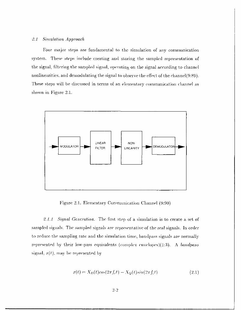
shown in Figure 2.1.

-7WMODULATOR -ppFILTER -00 LINEARITY -0,DEMODULATOR -00

Figure 2.1. Elementary Communication Channel (9:90)

2. 1.1 Signal Gcneration. The first step of a simulation is to create a set of

sampled signals. The sampled signals are representative of the real signals. In order

to reduce the sampling rate and the simulation time, bandpass signals are normally

represented by their low-pass equivalents (complex envelopes)(1:3). A baizdpass

signal, x(t), may be represented by

X(t) = Xj(t)co..s(2irf) - Xc(/),7i(27.f,1) (2.1)

where

x(t) ti6medomain signial

XD(t) =direct componen.7t

XQ(t) =quadrat tre componecnt

f,(t) =cenzterfrequency of the process

U~sing standard trigonometric identities, the bandpass signal can be equivalently

represented as

x(t) =R(t)cos[27wf't + 4)(t)] (2.2)

where

R~t) [X2L(t) + X2 (t)]1/2

The complex envelope of r(t) is then

Thlis representation of the signal is known as the complex low-pass representa-

tion. Use of the complex representation significantly redluces simulation time because

the center (carrier) frequency is not required in the simulation.

For a sampling frequency f, the Complex enivelope representation is(9:90)

.r(k -dt) .( i)J'epjw(L)k±j§( I)](2.4)

2-3

where

* ( k" ( rprs nits amplitude modulation

(P( k" (I ) r pr s is phase inodulation

i. ih rtlatire carrier frequency

I' i.l, I/nu saiql powcr

.f. - 1/',l! i.,/ tt o . mplin~g fr qur ncy

A" i. !/i sample index

The main c(ionsierdl loll ili select ilig the sampling frequency f, is the total band-

width required around the (halnel carrier frequency. In a digital communication

system, the bandwidth is determined by the frequency spectrum of the transmitted

symbol. .Nyquist's Sampling Theorem states that only 2 samples per symbol arenecessary to reconstruct the original signal. For simulation purposes, the sampling

frequency should be an even integer between 8 and 16(9:90). If the sampling fre-

quency is less than 8 samples per symbol, accuracy is lost; with more than 16 samples

per symbol, excess simulation time is used without significant gain in accuracy(9:90).

. .2 Filtering of Signals. The next consideration in the simulator is the

use of filters in the system. The primary purpose of system filters is to give an

acceptable tradeoff between desired signal distortion and interference from adja-

cent channels(9:91). The simulator requires a flexible capability to model different

gains/delays versus the frequency functions(9:91).

Efficient algorithms are necessary for a simulator because filtering tends to be

the most CIPU-intensive aspect of the simulation(9:91). There are three methods

usually used to simulate filter actions: 1) convolve the sampled signal with a stored

filter impulse response; 2) iultiply the discrete Fourier transform (1)T) of the

signal by the filter frequency transform function and take the inverse DFT to return

the signal to the time dorailn representation; and 3) operate oi the signal according

2-4

to the difference equation governing the filter(9:91). Direct convolution, the fiit

method, is rarely used because of the excessive CPU time required to perform the

computations. The DFT approach is the most general and commonly used method

to simulate the effects of filtering. However, for low order classical filters, such as

the Butterworth or Chebyshev, the difference equation method is quicker than the

DFT method.

2.1.3 (Than ucl Noin tiariis. Analytical approaches become complex, if not

impossible, to use when the systeiii model contains nonlinearities. Simulation is often

the only practical approach to perform system evaluation(9:92). Most simulations

of devices with abrui)t nonlinearities generate input/output tables to map input

values to output values. These lookup tables are used when the simulator encounters

abrupt changes to the input value and interpolation of the data points are used if

necessary. For gradual nonlinearities in the simulation, power series representations

of the input/output relationship are used(9:92).

2. 1 ./j Rccciver Struclun .s. The first module in the receiver structure is the

receiver front-end filter. At this point in the model the remaining steps in tile

simulation include the addition of noise, demodulation, and quantitative performance

evaluation(9:93). Performance evaluation would be measured by the signal to noise

ratio for analog systems and the bit error rate for digital systems(9:93).

Two types of simulations are used depending on whether thermal noise, usually

Gaussian, is added. The hybrid sinulation/analysis approach is used if thermal noise

is not added in the simulator. This approach uses simulation to obtain the statistics

of any other sources of -signal interference or distortion. The effect of thermal noise is

then added to the statistics and an average error rate is calculated(9:94). In the direct

simulation approach, thernual noise is added, demodulation is performed, and the

performance of the overall system is evaluated. For digital systems, error count ing is

required, th'erefore making these si 1nnlat ions inherently tiie-coisiiiing(9:94) The

2-7

Monte Carlo technique is a method of ensuring that simulating a certain number

of symbols will yield the estimated BER within a range of accuracy and a level of

confidence.

The demodulation and detection processes reduces the waveform to a number

which is then compared to a threshold. The decision process can be described in

relation to the probability densi tv functions (pdf) fo(v; T) and fl(v; ), of the input

voltage at the sampling instant r. The detection decision is made relative to the input

voltage at the sampling time T given that a "one" or a "zero" was sent. Deciding

a "one" was received when a "zero" was sent occurs when there is a large positive

excursion of the receive voltage from the value of a "zero". If the excursion of the

voltage is suflciently large to exceed the threshold voltage VT, an error will occur.

Sample densities are shown in Figure 2.2. These densities may, in general, assume

any shape and are not necessarily identical.

///

/ NI

VT (THIR ESHOLD)

Figure 2.2. Error Probability(3:155)

The probability of error, given that a one was sent, is

lProb[error/one-] £p = J ()d , (2. 5)

The probability of error, given that, a. zero was sent, is

2-6

Prob[error/zero] j-- p fo(v)dv (2.6)

1 he average probability is then

p - 7ipi + ToPo (2.7)

where

7 1 is the a priori probability of the symbol "one"

7wo is the a priori probability of the symbol "zero"

2. Montc Carlo Technique

The Monte Carlo method is basically an error counting technique. In other

words, the Monte Carlo technique estimates the probability of bit error by observ-

ing the number of error occurrences. Suppose that a "zero" was sent. Then the

probability of error is

o fo(v) (2.8)

This may be rewritten as

PO ho(v)fo(v)dv (2.9)

where ho is an error detector given by

{, 1, < V'.

2-7

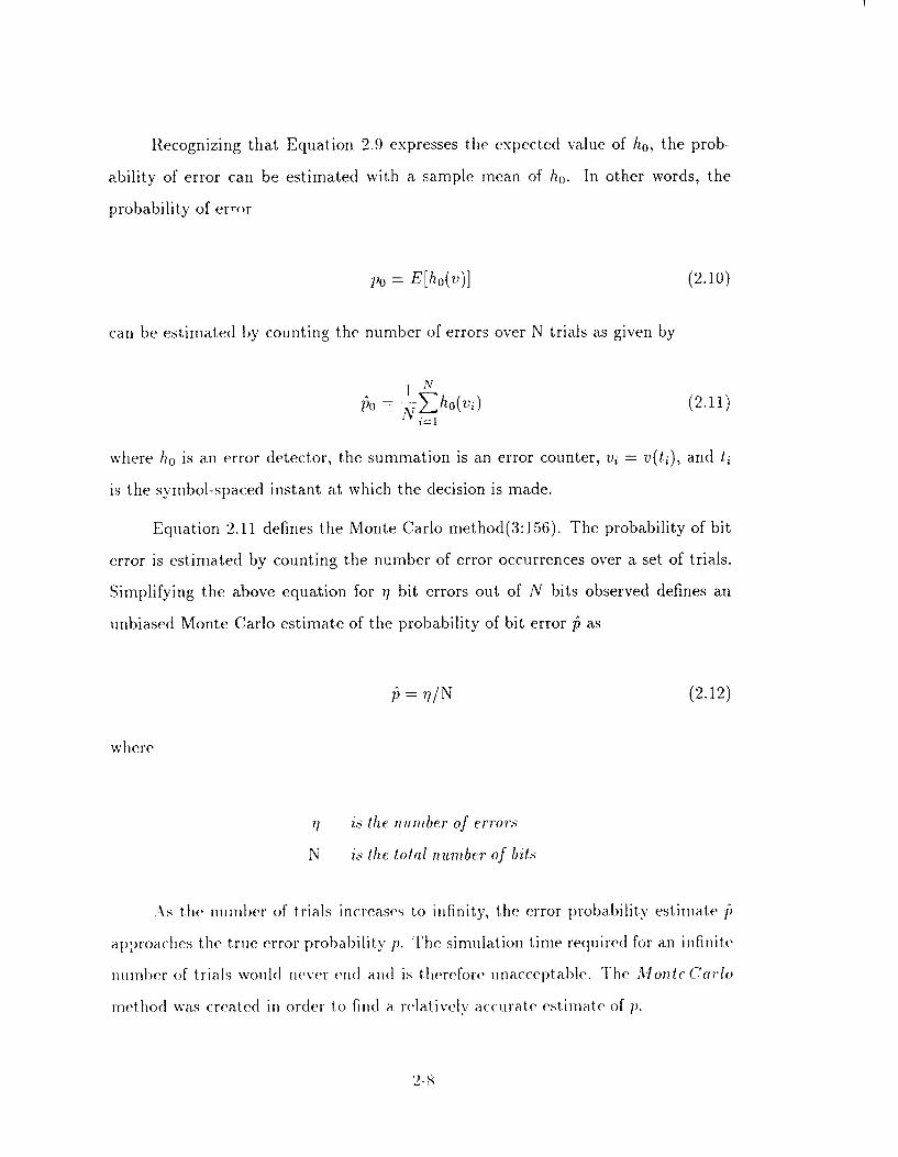
Recognizing that Equation 2.9 expresses the expected value of h0 , the prob-

ability of error can be estimated with a sample mean of ho. In other words, the

probability of er-or

p0 = E[ho(v)] (2.10)

can be estimated by counting the number of errors over N trials as given by

I N

P (2.11)N /i=1

where ho is an error detector, the summation is an error counter, vi = v(ti), and ti

is the symbol-spaced instant at which the decision is made.

Equation 2.11 defines the Monte Carlo method(3:156). The probability of bit

error is estimated by counting the number of error occurrences over a set of trials.

Simplifying the above equation for 7i bit errors out of N bits observed defines an

unbiased Monte Carlo estimate of the probability of bit error as

f) = 71/N (2.12)

where

71 is the number of errors

N is the total number of bits

As the number of trials increases to infinity, the error probability estimate f

approaches the true error probability p. The simulation time required for an infinite

number of trials would never end and is therefore unacceptable. The Monte Carlo

method was created in order to find a relativelv accurate estimate of p.

2-8

In the Monte Carlo method of estimating the probability of error p , enough

errors need to be counted to ensure that a degree of confidence can be assumed that

the error probability estimate it is relatively (lose to the actual error probability p.

The confidence level can be defined as(3:156)

P[h2 <p h,] =( - a) (2.13)

h - h12 is ith- confidence interval

(1 - a) is the confidence level

In other words, (1 - a) is the probability that the true value of the BER p is bracketed

by hl and h2. Figure 2.3 shows the number of trials that needs to be observed before

the estimate error rate lies within a desired confidence level of the actual error rate.

In general, a minimum of 10k+' symbols should be observed before there is an

acceptable degree of confidence in the error estimate j (3:157). This is equivalent to

a vertical slice on the chart where N = (Iok+ l ). Going across the chart at the 90%

confidence range shows that observing 10k+1 symbols defines a confidence interval

where the estimated error probability i is in the range of 0.51) to 2p. This interval

is considered acceptable(3:157).

Figure 2.4 illustrates the operations performed by a Monte Carlo simulation.

ihe input .x to the processor is a randtom variable of a. known probability density

function, fx (r). tUsing a finite number of observations, we want to estimate the

nuniber of errors occurririg iii y. The sorting operation is deciding if an error has

occurred. The output z7 is the number of errors.

However. ise of the coll vent iona I Monte Carlo technique is Ii itedI to error

prol)abilities in the region of -0 2 10' , anrid possibly 10- 1 (9:93). Verifying lower

2-9

10k 90 95

10 1 0 161+ 1

N, Total Number of Trials Observed

Figure 2.3. Confidence Bands When Observed Value is 10)-k (3:158)

error rates b~ecomes extremelyv time consuming b)causo- of the number of samples

he siulaor is requiiredl to generate. A Variation of the conventional Monte Carlo

method using Importance Sampling has been dlevelopedl to redluce the nulmb~er of

samples required, t hereby reducing the simiiulation timec.

2 3 Andid Alouji C arlo Tech nique [!sinq JnImortftnc( Sampl]ingl

T[he larige numibe r of samples requlired to be generated for a sinaill numtber of

emrsr to bec 'olil utedl m ake thle Mlonte Carlo meth1o0( iefficient . T he miajorit v of

lhe gener ated signtals do not, cause errors ( thle -imiport ant" event ). If th e noise is

zero- ruean (" laussianl for example, the iost, probalble value1 I.,/ero, alnd Zero will

2-1(0

THRESHOLD

INPU, xOUTPT, SORING OBSERVABLE, z

OPERATION

Figure 2.4. Sketch of Operations Performed with Conventional Sampling (6:17)

not generate an error. There is , t-ualn range of values centered around the mean

v, alue that also do not coitribute to error occurrences. The samples generated that

dto not indluce errors are, in effect, wasted. Implortance sampling is a imethod of

Making errors occur more frequently by a dleliberate (distortion, called biasing, of the

statistics of the underlying noise process that causes errors to occur(3:158).

The probability of error given a "zero" was sent, as shown in Equation 2.9, can

be rewritten as

Po /xuh(1v)I f0( v) '. (2.14)

where fo ( i') is t he bla.qcd denisity function. Noise samiples fromn ./ (r) wvill cauise tile

errors to occuir more frequeutly because, as shown later, fj illI be formned from1 0o

III such*l a wa v as to Mcrease th le noise pox\Tr(:159).

9- 1

The ratio

Wv(z) =f 0 (z)/fJ*(V) (2.15)

is calledI the wcight, or "unbiaser", of the function and the inverse of v(zv)

is called the bias of the function.

I" aton 2.14 can be rewritten as

Po Jho(v)w(z)fO(v)dv (2.17)

where hi*(v) is an error detector, not now based on a count of one as inI conventional

Monte Carlo, but now based on the weight wv(v).

As shown in Section 2.2, Equation 2.18 may be written as

Po E[ho*(v)] (2.19)

As before, the estimate of this equation cani be expressed as the sample mecan

iN.

Ni =1

IN.N S ~o~v )v' v~)(2.21)

N*i=i

2- 12

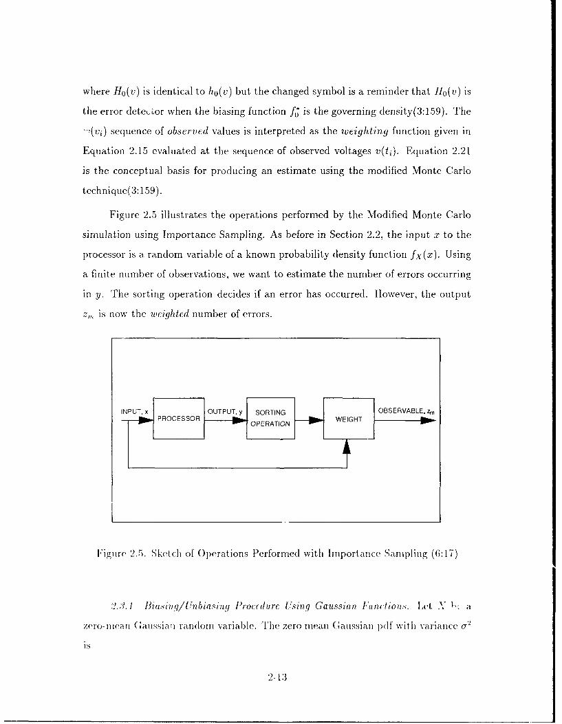
where Ho(v) is identical to ho(v) but the changed symbol is a reminder that Ilo(v) is

the error dete, uor when the biasing function fJ is the governing density(3:159). The

",(vi) sequence of observed values is interpreted as the weighting function given in

Equation 2.15 evaluated at the sequence of observed voltages v(ti). Equation 2.21

is the conceptual basis for producing an estimate using the modified Monte Carlo

technique(3:159).

Figure 2.5 illustrates the operations performed by the Modified Monte Carlo

simulation using Importance Sampling. As before in Section 2.2, the input T to the

processor is a random variable of a known probability density function fx(x). Using

a finite number of observations, we want to estimate the number of errors occurring

in y. The sorting operation decides if an error has occurred. However, the output

z, is now the weighted number of errors.

INPUT, x OUTPUT, y SORTING OBSERVABLE, Zm

. PROCESSOR . 1.1-0p OPERATION WEIGHT

lIigire 2.5. Sketch of Operations Performed with Importance Sampling (6:17)

2.:'?.I 13 Iisig/Unbiasing tProccdirc U/sirg Gaussian Functions. let V I-. a

zero-miean G a.,issian; random variable. The zero mean Gaussian d)(If with variance (,2

is

2-13

f(x) = (1/N 2/ Toq)exp(-x2/20,2) (2.22)

For importance sampling, the Gaussian noise pdf is changed to cause errors to

occur more frequently. The biasing function B(x) is defined as

f~x) f(x)B(x) = fx(x) (2.23)

where the variance o,2 of f(x) is unity and the variance a.2 of f*(x) is greater than

one so errors will occur more frequently. If f.(x) is used as the noise pdf rather than

the original fx (x), then more samples will come from the region of interest (the tails

of the pdf)(2:1918).

The biasing scheme suggested is (2:1920)

C

B(x) [fx(x) (2.24)

where the constants c and a are chosen such that the new density f, (x) has unity

area. This means that

J (x)&x (x) f(x)dx = 1 (2.25)

The a is optimized for the 13ER of a particular system using(2:1920)

-(2M + 1)+ /2M + 1)2 + 47'2(1 + 72)

0 1 -r = 2T 2 (2.26)

wxhere M is the nmnory in the systeni and T the threshold defined by T

-' (F2 ). This man,s that

2-14

C =(2.27)

The weighting function w(x) is given by f(x)/f*(x) for a single sample point.

From Equation 2.21, the BER is estimated by counting the errors and unbiasing

each count by the ratio of the input densities. For the case where there is several

samples per symbol and the input samples are independent, the weight of the noise

that caused the error to occur is given by(3:160).

Mwv(xi) = I f Y(xi-j,,)/f .(Xi-jA) (2.28)

j= 1

where fx and ft are single dimensional (assumed stationary) densities, i is the

symbol index, j is the sample index within the symbol, and M is the number of

samples within the symbol.

2.3.2 Estimation Error. Associated with simulation is the error of the esti-

mated value with respect to the calculated value. The number of samples required

to estimate P, by direct counting is(2:1922)

N > 1 (2.29)

where c is the normalized error of the estimated Pe. Rewriting Equation 2.29, the

normalized error is

c (2.30)

where 7, is the standard deviation of the estimate 1e.

2-15

When computer simulation has been chosen to evaluate a communication sys-

tem, it is important to choose a simulation software package that is both flexible and

accurate.

2.4 Siniulation Software Packages

Several software packages are now available for simulating communication sys-

tems. The features that make one simulation program a better choice for a particuar

application are not clear-cut(1:2). However, it is important to understand the fea-

tures that a communication simulation package should have, and a summary of

desirable features as identified by Balaban and Shanmugan (1) are listed below.

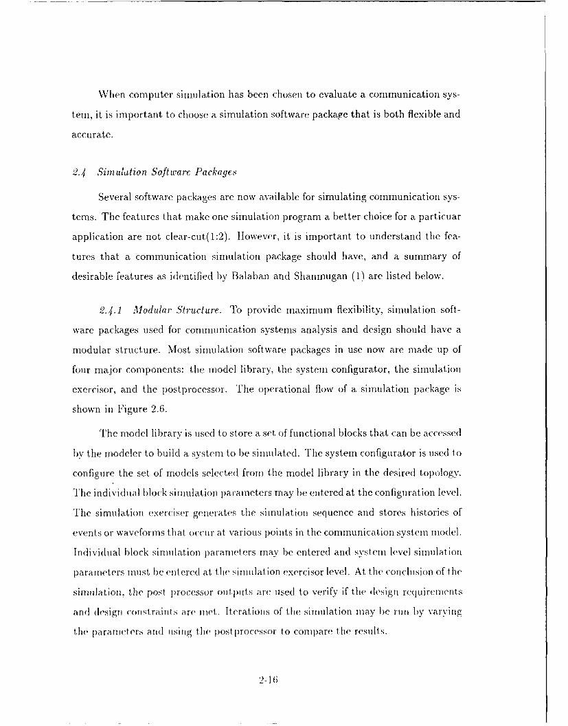
2.4.1 Modular Structure. To provide maximum flexibility, simulation soft-

ware packages used for communication systems analysis and design should have a

modular structure. Most simulation software packages in use now are made up of

four major components: the model library, the system configurator, the simulation

exercisor, and the postprocessor. The operational flow of a simulation package is

shown in Figure 2.6.

The model library is used to store a set of functional blocks that can be accessed

by the modeler to build a system to be simulated. The system configurator is used to

configure the set of models selected from the model library in the desired topology.

The individual block simulation parameters may be entered at the configuration level.

The simulation exerciser generates the simulation sequence and stores histories of

events or waveforms that occur at various points in the communication system model.

Individual block simulation pa.ranieters may be entered and system level simulation

parameters must be entered at the simulation exercisor level. At the conclusion of the

simulation, the post processor outputs are used to verify if the design requirements

and design constraints are nmet. Iterations of the simulation may be run by varying

the parameters and using the postprocessor to compare the results.

2- 16

TOPOLOGICAL SYSTEM DESCRIPTION(SIMULATION LANGUAGE OR GRAPHIC INPUT)

NEW

TOPOLOGY SYSTEM -S MODEL

CONFIGURATION LIBRARIES

COMPILED

SIMULATION

PROGRAMCS

PARAMETERS SIMULATION MODEL AND

PF A SYSTEMEXEREISOR PARAMETERS

S IGNAL OR EVENT

TIME HISTORIES

POST

PROCESSOR

1PERFORMANCE ANALYSIS,

GRAPHIC OUTPUT,ERROR RATES,TIME DELAYS,ETC...

F'igure 2.6. Operational Flow of a Simulation Package

2./4.2 Sintlation aii ! .)rogramming Language. The software used in the sim-

ulator should be written in a higher level programming language such as Fortran,

Pascal, or C. Illese languages, however, do not allow input to the simulator via block

diagrams. Therefore, to connect the block diagrams to the simulation exercisor, a

preprocessor simulation language is required.

2.4.3 Topological Configuration. The configurator of the simulator software

package should allow connection of the model functional blocks in any topological

2-17

configuration. This feature permits maximum configuration flexibility, however, it

may complicate the simulator software structure.

.. 4.4 Model Library. The usefulness of a simulation software package de-

pends heavily on the number of functional blocks contained in the model library.

The model configurator should allow unlimited nesting of the blocks in the model

library to permit any subsystem model to be built. The user should be able to write

his own model, and either enter it directly into the system model for simulation or

enter it into the model library.

2.4.5 Time and Event Driven Simulation. A simulator should be designed

so that processing can occur either at every "tick" of the simulation clock or when

identified events occur. For maximum flexibility, both options should be made avail-

able to the user. Provisions should be made in the simulator so that the user can

designate model blocks either as event driven or time driven.

2.4.6 Postprocessor. The postprocessor function of the simulator should en-

able the designer to view the results of the simulation. The postprocessor should

allow the users to draw direct cause-and-effect inferences about the system opera-

tion. As a minimum, the postpro(essor should perform functions of common test

instruments such as spectrum analyzers, and software utilities such as profilers of

resource utilization. Statistical analysis. as well as graphics display routines, are also

essential for the postprocessor.

2.4.7 ("ser Intrface. The sinilation package slOtld be user friendly. The

documllentation provided with the package should be comprehensive and understand-

able. On-liine do((inlation, such as -help", should be available and noncry!)tic to

the utser.

2-18

2.5 Block-Oriented Systems Simulator

The Block-Oriented Systems Simulator (BOSS) provides an interactive envi-

ronment for block oriented system analysis and design(12:1-2). The BOSS software

structure is shown in Figure 2.7. BOSS has a rich environment of block modules in

the model library. The supplied blocks are easily altered, enabling new blocks to be

designed. "Primitive" blocks may be interconnected to build a new block. These

new blocks may be added to the model library.

BOSS has a hierarchical method of building systems to be simulated. BOSS

performs consistency checking to ensure proper connectivity between all modules

and to verify valid input parameters are used.

When the system to be modeled is stored in the simulator, the parameters are

entered and the simulation is performed. The post processor displays the data in

various formats. The user decides what data is to stored by inserting probes into

the model.

BOSS runs under the VMS operating system on a DEC VAX Station or under

the UNIX operating system on the SUN-3 workstation(12:1-2). BOSS provides high

resolution bit mapped graphics (1024 x 864) and uses both a mouse and the keyboard

for inputs.

I-1)

Display

SimulaioManager

Post r 2..BBSlfockS iillr (217

III. Modeling of the System

The Block Oijented Systems Simulator (BOSS) provides for simulation-based

analysis and design of any communication system which can be represented in block

diagram forn(12:1-2). Simulation models of systems to be evaluated are built us-

ing a hierarchical block diagram approach. Once the system to be modeled is ex-

pressed in block diagram form, BOSS supports a time-domain, or waveform level

simulation( 12:1-2).

To build a system to test and verify the Monte Carlo technique and Importance

Sampling using BOSS, it was decided to use a simple, real-valued Binary Phase Shift

hey (BPSK) system o, c aing at baseband. Built-in BOSS modules were used in

the system wherr , ,ossible. Changes mnade to existing BOSS modules were kept

to a minimu_. BOSS modules, systems, or parameters will be capitalized to set

them apart from generic terms. This chapter will begin with building the basic

BPS! system and will then evaluate the system using the conventional Monte Carlo

method.

3. 1 BPSK System Decomposition

The first step in the BOSS modeling process is to perform a top-down de-

composition of the system. The blocks required for a BPSK system are the data,

generator, the BPSK modulator, the channel, and the BPSK demodulator. Added

to the model will be an error detector to identify errors and provide the estimated

BER.. The next sections will discuss the modeling of these blocks.

3. 1. 1 Data (G3m rator. 130SS provides a digital data generator in the model

library. lhe generator in BOSS is called RANDOM DATA and is located under the

group I)I(; ITA , S()il R( S. Figure 3.1 shows the internal modules that imake u1p

the data generator mo(dIule.

3:1

RANDOM DATA

IMPLSECONST >

El T R A I N >V EI G E N

>

O# 1 OUTPUT

Figure 3.1. RANDOM DATA Internal Modules

RANDOM DATA generates a random binary bit stream (logical "true" or

"false") at a specified bit rate and probability of false. RANDOM DATA requires

the parameters shown in Table 3.1 to generate the bit stream.

Table 3.1. RANDOM DATA Parameters

ISEEDPROBABILITY OF FALSE

BIT RATE

The parameter ISEEL) is the seed of the underlying random number generator.

The generator has a uniform distribution. ISEED will be renamed DATA GENERA-

TOR SEED to differentiate between the different seeds in the model. This parameter

will be passed up to the system level because the DATA GENERATOR SEED will

be one of the parameters varied to determine thie estimation error. The parameter

PROBABILITY OF FALSE will be set internally in the RANI)OM )ATA module

to be 0.5. This setting ensures random data is output from the niodule. The pa-

rameter BIT IRATE, will be renamied SYMBOL RATE and will be passedt up to the

svstei rnolel.

3-2

3i.1-0 I3PSK M1odulator. BOSS provides a I3SPIK modulator in the model

library. The modulator in BOSS is called BPSK MOD and is located under the

group DIGITAL MODULATORS. Figure 3.2 shows the internal modules that make

uip the modulator module.

BPSK MOD

1 LOGICAL COMPLEX> TO >SPECTRAL>[:] NUMERIC ELSHIIFTER

1# 1 BPSK MODULATED SIGNAL 0# 1 BPSK MODULATED SIGNAL

Figure :3.2. I3PSIK MOD Internal Modules

The B3OSS module BPSK MOD modulates the input bit stream to the constel-

lation of (1,0) and (-1 ,O). In1 order to set the bit error rate to a dlesired value later,

the values of the constellation were changedl to be (TRUE VALUE,0) and (FALSE

VALUE,0). Both constellation values were set to be real numiiber-s. Also, because the

simu11lationl will be run at lbaselbandl, the COM PLEX S1PECTR AL Sill PIER block

was deletedl. To (lifferentiate thle user generated m11(1111e from1 tHie 130SS niodule.

the new mnodlule is savedl as Bl'SIK MOD)ULATOR in the group MISCELLANEOUS.

I3l1S1K MODULATOR, is shIown lin Figure 3.3. Thils module out put, is connectedl to

1)0thl tlI Cliecannel input anmd to tHie uncorrup~tedl i iut of thie BPlSlK demodulator.

BlPSK MOD)ULATlOR reqires t lie Laaivt ers shiowni in Table 31.2 to generate time

miolilatedl lit streaml.

TlIme pa ranmet ers T lW I VA 1.111 and IK SFVA 1.1 1' Set the aiillituldes of I '

logical (Iata generator omitpm its. IA L\fS 1K VA 1 was set in1ternial lY III Tiodule to 1e

3-3

BPSK MODULATOR

LOGICAL1 ~ >TO1[E NUMERIC

1# 1 BPSK BINARY INPUT 0# 1 OUTPUT

Figure 3.3. BPSK MODULATOR Internal Module.

Table 3.2. BPSK MODULATOR Parameters

TRUE VALUEFALSE VALUE

the negative of TRUE VALUE. TRUE VALUE was passed tip to the system- level

alI( will be use(I to set uip a p~redictedl BER.

3... I ?Olannci. BOSS does not provide a, channel that was dlesiredi for this

miodel "I'e channel for this model requires a real-vahuedl white nioise( generator

and aii adder BOSS providles a generator called GAUTSSIAN RAN-GEN under the

group NOISE AND) INTERFERENCE. The 13OSS module GAUSSIA N ?AN-GEN

gences l valued Gaussian wite noise wit h alJ ustable nii~ andh va iauce. Ta ble

3.3 shoxo s thle v1ra mieters requli redl to gernerat ed thle Gaussin uiow~.

Talhe 3.3. GA[USSIAN ?A N-GEN Pairamiet rs

ISEED,%I."'AN

VA I IIA N('I

3- 1

The parameter ISEED was renamed NOISE GENERATOR SEED). VARI-

ANCE and NOISE GENERAFOR SEED) were passed up to the systcun level. NOISE

GENERATOR SEED) must be a large 0(1( integer and will be varied to (determine the

estimation error. VARIANCE will be set to a value of one for conventional Monte

Carlo and will be changed] for the Importance Sampling module. MEAN was set to

0.0 and stored in the miodule.

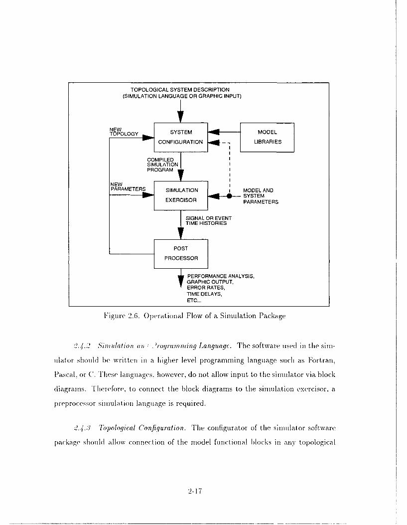
To model the channel, a module called CHANNEL was generated. This miod-

ule will input tne BPSIK1. signal, add Gaussian noise to the signal, and output the

cor- _4ed BI"SK signal. Figure 3.4 shows the internal modules of the user gener-

ated1 CHANNEL. CHANNEL parameters are the same as GAUSSIAN RANGEN

parameters shownv in Table 3.3.

CHANNEL

I> +

1# 1 INPUT 0# 1 OUTPUT

Figure 3.4. CIHANNEL Internal Modules

.. 1I3I'.SA DcindiIlUlor. 13OSS provides a, PSIK deiodtilator and er-

ro)r coun ter Mi the model library. '['liis iodlule is called P51(i) F1IKM()11AND

ERRIOR C( 0111iR and is located under the group lFIOMLTPS

lPS1K D1)M01) AN NI BlROR .(() 1T' T1. inmternal modu1 les a me slowin Mligure :3.5.

H owever, thle rn1odl1le slippl ied Iv RO SS is conifigiiie(I for (01mplex signals and was

3-5

changed to work with real signals. The module was further changed to move the er-

ror counter outside the module so that changes to incorporate Importance Sampling

would be easier. The error counter changes are discussed in the next section.

PSK_ DEMODAND ERRORCOUNTER

I#2E RECIVE PS

Figr 3,SDE NUMBER I>COUNTER

TAT! CHED FILTERCED MILDEODULTOR !. I"NUMBER

Ei- PosrroN -. _INSYMBOL v

1# 1 TRANSMITTED PSK

1# 2 RECEIVED PSK

Figure 3.5. PSKDEMODAND ERROR-COUNTER Internal Modules

The BOSS m-odule PSK MATCHED-FILTER DEMODULATOR internal mnod-

ules are shown in Figure 3.6. The integrate and dump integrator integrates over one

symbol interval and dumps the output at the end of each symbol. The PSK DE-

TECTOR quantizes the output of the integrator to the nearest constellation point.

In other words, for BPSK, the PSK decides which constellation point the received

symbol represents by checking whether the integrator output is greater than or less

than zero. Removing the IMAG OF COMPLEX and REAL OF COMPLEX mod-

ules, one INTEGRATE A Nl)I)IIM P module, and adding a constant generator were

the changes necessary for the denodulator to function for real-valued signals. The

constant generator was required for the MAKE COMPLEX module input because

3-6

the PSK DETECTOR requires a complex signal. The modified module was saved

as REAL BPSK MATCHED FILTER DEMOI)ULATOR in the group MISCELLA-

NEOUS and is shown in Figure 3.7.

PSK MATCHED FILTER DEMODULATOR

> ---------- = OF >INTEGRATE" I'A...-MP >AND-DUMP>F MKEL ,°dI-- SL . . I[DETECTOFP

Th R INTEATER D U R u iteprmtr o i >ANDDUMPA

Ei POSITION Pd -n ---] INSYMBOIf OR

I-IDIRAC r

DELTA

1# 1 RECEIVED PSK STREAM 0# 1 DEMODULATED PSK

Figure 3.6. PSK MATCHEDFILTER DEMODULATOR Internal Modules

The REAL BPSK MATCHED FILTER DEMODULATOR module requires

the parameters shown in Table 3.4. The MAKE COMPLEX IMAG INPUT was set

to zero and stored in the module. Because the system is real-valued and channel

phase rotation does not occur, CHANNEL PHlASE ROTATION (DEG) was set to

zero and stored in the module. PSK CONSTELLATION FIRST ANGLE ()EG)

was set to 180 degrees and PSK MOI)ULATION ORDER was set to 2, both for

BPSK, and stored in the module. The model has no delay elements between data

generation and the input to the demodulator, therefore TIME I)'LAY TO INPUT

(SEC) was set to zero. SYMBOL RA'TE was the only parainelter carried up to tie

system level.

3-7

REAL BPSK MATCHED FILTER DEMODULATOR

> II>'INTEGRATE> AK

CONSTANT11

LJLDELTAc oP

I# 1 RECEIVED BPSK STREAM O# 1 DEMODULATED BPSK

Figure 3.7. REAL BPSK MATCHED FILTER DEMODULATOR InternalModules

Table 3.4. REAL BPSK MATCHED FILTER DEMODULATOR Parameters

MAKE COMPLEX IMAG INPUTCHANNEL PHASE ROTATION (DEG)

PSK CONSTELLATION FIRST ANGLE (DEG)SYMBOL RATE

TIME DELAY TO INPUT (SEC)PSK MODULATION ORI)ER

3-8

The changes were made to PSK]DEMODAND ERRORCOUNTER and

stored as BPSK DEMODULATOR under the group MISCELLANEOUS. The BPSK

DEMODULATOR module is shown in Figure 3.8. Again, the only BPSK DEMOD-

ULATOR parameter to be passed to the system level is SYMBOL RATE.

BPSK DEMODULATOR

STAGE MAKE SYMBOLDELAY >OP NUMBER

2 MATCHED 1> |

I# 1 TRANSMITTED BPSK 0# 1 TRANSMITTED DETECTED ABPSKI# 2 RECEIVED BPSK O#02 RECEIVED DETECTED BPSK SIGNAL

Figure 3.8. BPSK DEMODULATOR Internal Modles

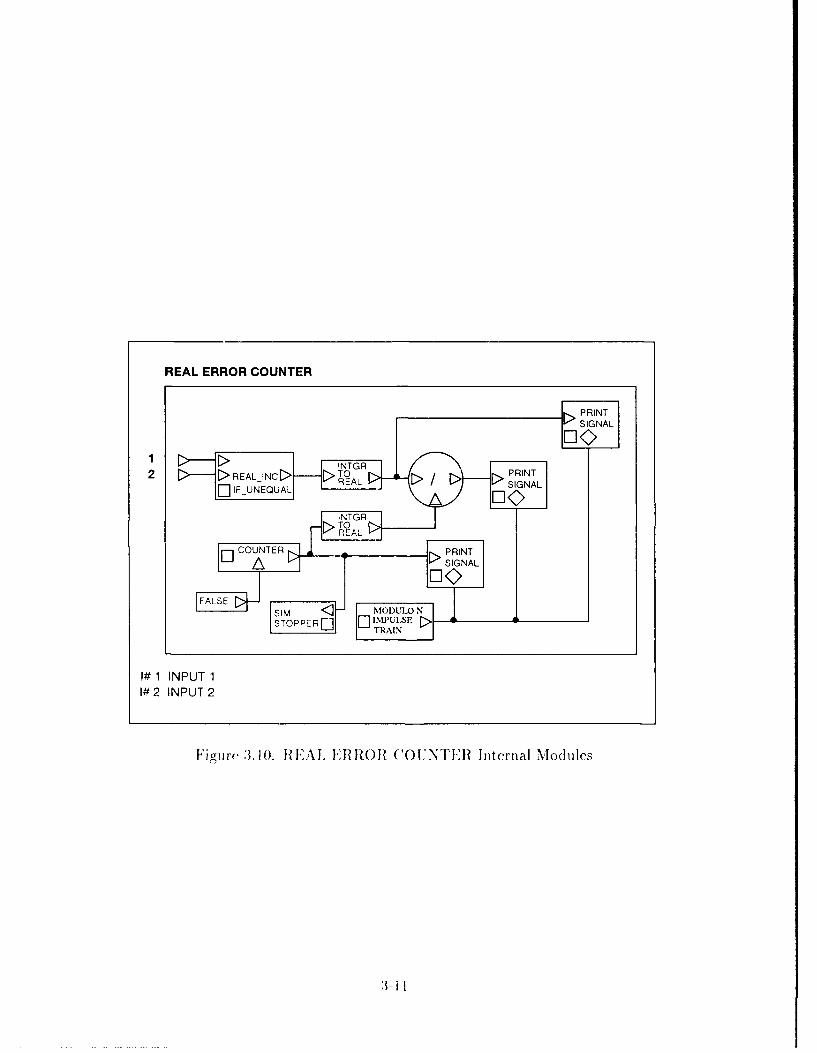
3.1.5 E, rror Detector. BOSS provides an error detector in the library. The

error detector is located under the group DEMODULATORS - INTERNALS. Added

to the BOSS supplied error detector was a print module so the output data would

include the BER calculation. Also added was a biock to stop the simulation when a

certain number of symbols were counted. The simulation stopper module was stored

as SIM STOPPER and is shown in Figure 3.9. The altered error counter was stored

as ?EA, I,' RROR COTTNTER and is shown in Figure 3.10. This niodule requires

an enable which is added as shown in Figure :3.11 and was stored as BPS!K E ItOI

3-9

COUNTER. The enable is required so the error counter will only be active for the

sample at the end of the symbol rather than active for every sample.

SIM STOPPER

l#TG I INPUT

Figure 3.9. SIM STOPPER Internal Modules

The BPSIK ERROR COUNTER module counts the number of times its two

inputs are unequal. The module prints the number of errors, the calculated I3ER,

and the number of symbols. BPSIK ERROR COUNTER requires the paramneters

shown in Table 3.5.

Tab~le :3.5. I3ISIK ERROR COUNTER Parameters

PRINT ESTIMATE MODULOSIM STOPPER NUMBER OF SYMBOLS

BIT RATESYMBOL FOR SAMPLE TIME

TIME DELAY TO INP~UT (SEC)

TIME" DELAY TO IN P1 T is thle jnmber of secoi(15 of (delay betweeii tratis-

mission of the first bit andl that li, appearig at the input of the denioduitor. T I1

DI) LAY TO IN P1T Ni as set to I < eci1s eas 1h niltegrat aIldm Ilte

de(-lays te i(,gnal by one symbiiol dii rait~in. 1) 11 INT 1EST I M AlE 10 (0 1) (. 11' Is a11 'tin1iit

t hat (let eriities after hiow ii ianv saij)les the I l E . iii iiber of sviibls 05 '( id I ilib r

31- i1)

REAL ERROR COUNTER

2 >RELINC >REL > />SIGIGNA

>~3 I IG

BPSK ERROR COUNTER

I ERROR2 COUNTER

[POSITION

IN NSYMBOL >

I# 1 INPUT 1I# 2 INPUT 2

Figure 3.11. BPSK ERROR COUNTER Internal Modules

of bits are calculated and saved. SIM STOPPER NUMBER OF ERRORS is an

input that terminates the simulation when a certain number of symbols are counted.

PRINT ESTIMATE MODULE and SIM STOPPER NUMBER OF ERRORS were

passedt up to the system level.

3.2 BPSK Systcn

The modules described in Section 3.1 are connected to form a BPSK system

model. This model was named BIPSK SYSTEM and stored in the group SYSTEM.

Figure3.12 shows the interconnedting of the modules. Table 3.6 shows the parameters

required by BPSISIK SYSTEM.

The parameter STOP-TIME specifies the maximum value of time (in seconds)

for the simulation. l)T is the time between discrete simulation signal samples (in

seconds). The other parameters have been presented in previous sections.

3.2.1 Dtcrmininq ISK Sysltcm lnicrnal lParamctcrs. Values for the pa-

rameters listed in Table 3.6 remain to be determined. STOP-TIM 1 is not important

3-12

BPSK SYSTEM

RANDT

PRINLT ETMTEMDLSYMBOL RATE(lIZVARIHANE

NI~OISER ENUMEATR OFSEDOL

VREIACE;NOISE'~ G ENER HATO)R S1KEl)D

3~- 13

to this system because the simulations will be stopped by the symbol count, riot by

the simulation clock. Therefore, the value of STOP-TIME was set to 1010 seconds

to ensure the simulator will run until enough symbols are counted. SYMBOL RAF]

for this simulation is arbitrary, so a symbol rate of 1000Hz will be used for all simlu-

lations. DT is the time between discrete simulation signal samples (in seconds). As

explained in Section 2.1.1, the signal will be sampled at a rate of ten times the sym-

bol rate, or 10 . seconds. SIM STOPPER NUMBER OF SYMBOLS and PRINT

ESTIMATE MODULO are parameters that will vary for different simulations and

will be determined later. NOISE GENERATOR SEED and DATA GENERATOR

SEED will be the values shown in Table 3.7. Parameter values for VARIANCE and

TRUE VALUE determine the expected system BER and will be developed in the

next section.

Table 3.7. NOISE GENERATOR SEED and DATA GENERATOR SEED Values

RUN NOISE GENERATOR SEED DATA GENERATOR SEED1 1,599,999,999 1,899,999,9992 1,699,999,999 1,999,999,9993 1,799,999,999 2,099,999,9994 1,899,999,999 1,299,999,9995 1,999,999,999 1,399,999,9996 2,099,999.999 1,499,999,9997 I1,299,999,999 1,599,999,9998 1,399,999,999 1,699,999,9999 1,299,999,999 1,899,999,99910 1,199,999,999 1,999,999,999

3.2.2 )d crinining Systen BER. To establish baseline parameters for com-

paring the estimated BIIR with the calculated BER, the expected system I31'R had to

be determined. The BE ,l for an antipodal 3PSIl\ svsten is calculated using( I 1:156)

tR ? =Q ( , ) (3.1)

:- 14

where

E6 is the energy per transmitted bit

No is the white noise power spectral density amplitude

and Q(-) is the well known complementary error function that is tabulated in many

communication texts and is defined by

Q(z) 1 / e=-dt (3.2)

3.2.2.1 Determining Energy Per Bit, Eb. Assuming equal energy sig-

nals, the energy per bit Eb is(11:157)

Eb = Is 2(t)dt = 2 s(t)dt (3.3)

LFor BPSK, s(t) is the bit amplitude A. Also, for antipodal BPSK signals,

s2(t) = .s(t) = s2 (t). Therefore, the energy per bit Eb is given by

Eb = A 2dt = A 2T (3.4)

3.2.2.2 Determining Noise Factor No. The noise factor No is deter-

mined by the value of VARIANCE entered and the simulation bandwidth. The

simulation bandwidth B, is a function of the sampling rate f,, where

B, -- 2 (i)T f, (:3.5)B 2 = DT

and is shown M Figure 3.13. The power, or variance (rN, in a. zero-mean, real-valued,

(;aussian randoni variable within the similation bandwidth Bs is found using

3- 15

f2 /~~2 cf f [/2 ( N 0 ) _f = ofl (36N f,2 GN(f)df = f/2 ) df 2 2 VARIANCE (3.6)

NOISEPOWER

G (f)

-- /2 0 A12

Figure 3.13. Simulation Bandwidth of a Gaussian Random Variable

The value of No is found from Equation 3.6 as

2(VAR lANCE)N, = 2(VARIANCE)(DT) (3.7)

3.2.3 MWS, SYSTEM Simulation lParam etcr Determinat ion. The BPSK SYS-

TIEM system internal parameters have been determined. Next. the system will be

3- 16

baselined using the conventional Monte Carlo technique. The system parameters

remaining to be determined are shown in 'Fable 3.8.

Table 3.8. BOSS SYSTEM Parameters Remaining To Be Determined

SIM STOPPER NUMBER OF ERRORSPRINT ESTIMATE MODULO

VARIANCENOISE GENERATOR IMAGINARY SEED

NOISE GENERATOR REAL SEEDTRUE VALUE

DATA GENERATOR SEED

The performance of the Monte Carlo techniques are to be evaluated by compar-

ing the estimated BER against the calculated BER. A desired calculated BER of 10 -

was chosen. This BER value was chosen so the simulation time of the conventional

Monte Carlo technique would not be excessive. VARIANCE and TRUE VALUE

(the hit amplitudes) determine the system BER. The parameter value VARIANCE

was chosen to be one because the the calculations are made easier in the Importance

Sampling section. Therefore, the bit amplitudes will be set to determine the system

BER. The value for TRUE VALUE remains to be determined.

After combining Equation 3.7, Equation 3.4, Equation 3.1 and simplifying, the

BER mav be rewritten as

BF? Q (VARANC)(I)T) (38)

Solving Equation 3.8 for the bit amplitude A yields

4 (VARIANCE)(DT) [Q-(I1?)] (3.9)

Stibstittiting in the known parameter values vields

3-17

A /(1) 10-4)_(1- [Q- 1 (10- 5 )] - 1.349

3.3 BPSk SYSEM I' erificatlion

The BPSK SYSTEM was simulated using the parameters previously disci.,uscd

to determine the estimated BER and estimation error. Ten simulations were ran

using the seed parameters listed in Table 3.7. The results of the runs are shown in

Table 3.9. All simulations took about 2 hours and 54 minutes to run.

Table 3.9. BPSK SYSTEM Using Conventional Monte Carlo Techniqtie Results

RUN ]:e (10-5)

1 1.402 1.003 1.604 1.305 1.706 1.30

7 1.208 1.20

9 1.3010 2.00

The statistics of the BPSK SYSTEM using conventional Monte Carlo tech-

niqi(es are shown in Table 3.10. According to Shanmugan(2:1917), this estimator is

"good" because the estimator error c is less than 1.

Table 3. 10. IB['SI SYSTEM Using Conventional Monte Carlo Technique Stat istics

FP,(1O- 5 ) 7-a (10-11) Tro,(10- 6 )

1.40 0.84 2.90 10.29

1' n(' xt, cliapter will develop tfhe modhdes for using the Modified Montie (adlo

teclul(iqii1c ,lsing llportan,ce Sampling.

3-18

IV. Implementing Importance Sampling

Most of the BPSK System model developed in the previous chapter is un-

changed using the Modified Monte Carlo technique with Importance Sampling. Mod-

ules to implement Importance Sampling will be new modules that eithe replace

existing modules or are added to the system model. The new system will be called

MODIFIED BPSK SYSTEM. This chapter will begin with building the new mod-

ules, incorporating the new modules into the system, and then evaluating the new

system as the performance compares with the old system.

4.1 Modified BPSK Syste' Decon position

MODIFIED BPSK SYSTEM requires a biased function generator, a weight

generator, and an error counter to calculate the estimated BER. The biasing proce-

dure is implemented by changing the VARIANCE parameter in the module CHAN-

NEL. The unbiasing procedure, however, requires adding a module for calculating

the error "weight" used for unbiasing the error count value. An error counter must

be added that will accumuiate the error weight sum and use that sum for calculating

the Importance Sampling estitmated BER.

4.1.1 Biased Noise 1'nnction. The biasing function B(x) was shown in Sec-

tion 2.3.1 to be

,f'(x)3(r) (.1)

The biased noise function suggested is of the form(3: I l

.f.(,) = c.f"V(7)/[fv(,)]" (.1.2)

4- 1

where c and a are constants to be calculated so the area under the pdf is one.

The equations to determine the constants c and a are shown as Equation2.27 and

Equation2.26, respectively.

Equation 4.2 represents the new noise to be added to the BPSK signal in

the channel module. Equation 2.26, with M = 10 being the number of samples

per symbol and T = 4.3, yields a = 0.605. Equation 2.27 shows that c = 0.13.

Substituting these values into Equation 4.2, the new noise pdf is

f (2n) = 0.25exp(-0.1975x 2) (4.3)

This Gaussian pdf has a variance of 2.53.

The previous module CHANNEL did not need to be modified to generate the

biased noise function. VARIANCE was again passed up to the system level.

4.1.2 Weight Generator. The weighting, or unbiasing, function is represented

by(4:69)

w(x) - f(x)(4)?x =f Wx (4.4)f*(x)

This simplifies to(4:69)

w(x) =(-/u)cxp[-(1 - a 21/a)(x'12)] (4.5)

Equation 4.5 repriesents the function that determines the weight of one noise

sample within a svrbol interval. 'lIh module to generate this weight function is

shown in Figure 1.1.

WEsI(;IiT G;ENE ATO I? req iiires the parameters shown in Table 4.1.MEAN

was set to 0.0 and VAIRIANCE was set to 1.0. ISEEI) was renamed NOISE (;N-

I:ATR() SE'l) aind was passed ii1) to thw system level.

41-2

WEIGHT GENERATOR

El ASIN>x>RAN-GENt X

0# 1 OUTPUT

Figure 4.1. WEIGHT GENERATOR Internal Modules

Table 4.1. WEIGHT GENERATOR Parameters

VARIANCEMEAN

VARiIAN(!'EMEVAN

This weight generator outputs a value for the noise at one sampling instant.

Equation 2.28 shows that the weight of the noise for one symbol interval is the

product of the weights of each noise sample in that symbol. WEIGHT FUNCTION

GENERATOR, shown in Figure 4.2, takes the value of each noise sample, multiplies

the value for 10 samples (one symbol), and outputs the value. Each SAMPLE

&-HOLD module samples the value at the symbol fraction shown in the input to

each SAMPLE &-HOLD. The TEN INPUT MULTIPLIER multiplies the inputs and

outputs the product after 10 samples have been taken.

WEIGHT FUNCTION GENERATORSSAMPLE

-HLD

GENERATOR01 >INU

> MULTIPUER

> --

SAMPULEPIE

0# 1 OUTPUT

Figure 4.2. WEIGHT FUNCTION GENERATOR lnteral Modules

WEIGHtT FtNCTION G'ENEtRATOR requires the paranieter~s s hown iTable

41.2. NOISE, ( l"NIM[AT()[ SFEEID will again be passed i ) to the systein('e to be

4-4

varied to determine the estimation error. VARIANCE and SYMBOL RATE (HZ)

will be passed to the system level. TIME DELAY TO INPUT (SEC) will be set

to 0.0 because there is no delay elements between the sample generation and the

input to the SAMPLE &-HOLD module. SYMBOL FRAC FOR SAMPLE TIME is

the parameter that determines which noise sample within a symbol each SAMPLE

&-HOLD module samples. The SYMBOL FRAC FOR SAMPLE TIME parameters

are entered for each module that inputs to each SAMPLE &-HOLD MODULE.

These values range from 0.0 to 0.9 in increments of 0.1 and are shown for each

module on Figure 4.2.

Table 4.2. WEIGHT FUNCTION GENERATOR Parameters

NOISE GENERATOR SEEDVARIANCE

TIME DELAY TO INPUT (SEC)SYMBOL FRAC FOR SAMPLE TIME

SYMBOL RATE (HZ)

4.1.3 Importance Sampling Error Counter. Once the weight for the noise in

each sample has been determined, the error counter must sum the values of the

weights when each error occurs. The estimated BER is determined by dividing the

weight sum by the number of transmitted symbols.

l"igure 4.3 shows the internal odu!es of the error counter that determines

the estimated BER using Importance Sampling. The module =REAL compares the

two inputs and determines if they are equal within a, parameter called ALLOWE1)

ROUNI)OFF FRACTION. If the inputs are equal, this Inodle outputs 'true', and

if the inputs are unequal, this module outputs 'false'. LOGICAL TO NIMERIC

converts the true or false outputs frorn tlie compare miodule into numerical outu)lts.

Ihe out put, is set to 0.0 when tihe inputs are equual, and 1.0 whien tlie inuputs are

uneq(ua.l. The nlwiltiplier module multiplies tl" ('rror weight )y 1.0 wlien an error

lhas occured and the Ii NNIN( SN ru()(1dile adds and stores the error weiglit sun.

1-5

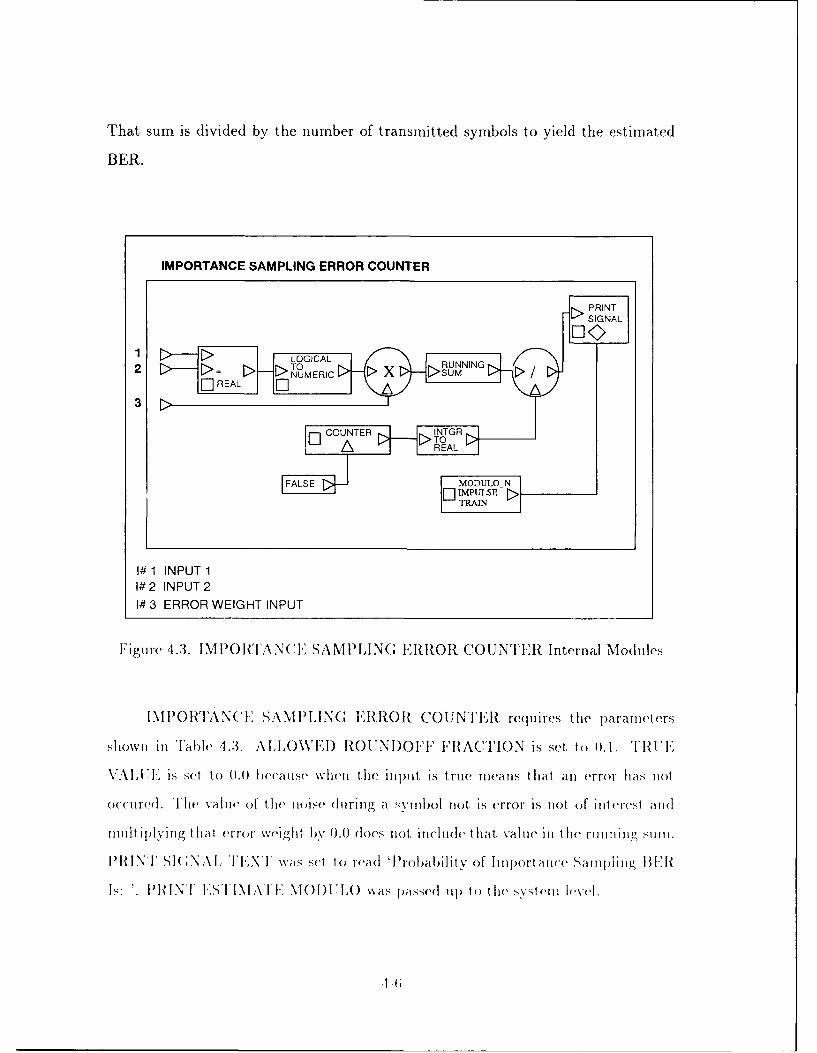
That sum is divided by the number of transmitted symbols to yield the estimated

BER.

IMPORTANCE SAMPLING ERROR COUNTER

2~~~~~~ PRINTJM RI ~ > U

I1 INU 1 IA2 INP=UT28 ININ

I3 ERRORTEIN WEG TRN U

Figue 43. IPORANC SAMLIN >TRORC NTRntrlMous

IMPPTAN('F A I PLIG lRRI{ OUTERreuirs he ~REALer

show in able4.3.A LOWLI ROII)OF EliACONDsUeLO 01 III''vA I Fis et o 00 Iwea se henI le ii pi~IUE asta nerrhsio

IIMl S( ;A I NE SAsPIN setM toNTI redeqo~blivo urs alic aalfJlic IIKI

Is,: '. IPlRINT' IK")il\IA'lIK \101)1 L() was passed up1 to thle sysleli level.

4.2 Modified BPSK System

'The BPSK system developed in Section 3.2 was modified to include the modules

developed in Section 4.1.3, Section 4.1.2, and Section 4.1.1. The model was named

MODIFIED BPSK SYSTEM and stored in the group SYSTEM. Figure 4.4 shows

the interconnecting of the modules. Table 4.4 shows the parameters required by

MODIFIED BPSK SYSTEM. All of the parameters listed have been covered in

previous sections.

4.3 MODIFIED BPSK SYSTEM Testing

MODIFIED BPSK SYSTEM was simulated using the parameters shown in

Table4.5. NOISE GENERATOR SEED and DATA GENERATOR SEED were var-

ied as shown in Table3.7.

Table4.6 shows the results of the tests. The results are obviously not what

were expected. The model has been extensively reviewed, rebuilt, and tested. Good

estirnated BER values were never given by the MODIFIED BPSK SYSTEM. Chapter

5 will speculate why the system does not work and suggest some further testing that

could be performed.

'Table 4.3. IMPORTANCE SAMPLING ERROR COUNTER Parameters

ALLOWED ROUNDOFF FRACTIONTRUE VALUEFALSE VALUE

PRINT ESTIMATE MODULOPI INT SIGNAL TEXT

4-7

MODIFIED BPSK SYSTEM

MGENERATO

Table~ 4..BOIFIED >H>S SYSEMDPARmtr

VARIANTANE

NOISE ~GENERATORI

II)TAE INUEFR OFSYMBI L

PRIN ESIMAE 4-UL

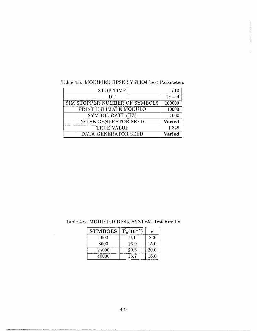
Table 4.5. MODIFIED BPSK SYSTEM Test Parameters

STOP-TIME lelODT le-4

SIM STOPPER NUMBER OF SYMBOLS 100000PRINT ESTIMATE MODULO 10000

SYMBOL RATE (HZ) 1000NOISE GENERATOR SEED Varied

TRUE VALUE 1.349DATA GENERATOR SEED Varied

Table 4.6. MOI)IFIED BPSK SYSTEM Test Results

SYMBOLS t0 (10- 5 ) c

4000 9.1 8.38000 16.9 15.0

24000 29.3 20.0'10000 35.7 16.0

41-9

V. Conclusions

This chapter will discuss the test results of the system using conventional

Monte Carlo technique and the system using modified Monte Carlo technique with

Importance Sampling. Furthcr, possible reasons for the modified system not working

are given.

5.1 Conventional Monte Carlo Technique

BPSK SYSTEM was tested using the modules and parameters as explained in

Chapter 3. The results of the test are shown in Table 3.9 and Table 3.10. The average

of the estimated BER is 1.4X10 - . The mean was well within the Monte Carlo

expected value of 0.5X10- to 2.0X10 - '. Further, the estimator error statistic e was

0.29. Again, this was well within the range of 0 to 1, which shows the conventional

Monte Carlo technique is a good estimator of the actual BER.

However, conventional Monte Carlo technique requires the simulator to gen-

erate 10k+ 1 symbols for a BER of 10 k . For simulations of low probability events,

the time for conventional Monte Carlo techniques become excessive. An extension of

the conventional Monte Carlo technique is to use Importance Sampling. Importance

Sampling is a method of reducing the number of required symbols while retaining

the confidence levels of conventional Monte Carlo. The results and discussion of

implementing Importance Sampling follow in the next section.

5.2 Modified Monte Carlo Technique Using Importance Sampling

MODIFIED BPSK SYSTEM was built to include Importance Sampling by

modifying the BPSK SYSTEM model. The MODIFIED P'SK SYSTEM model

and parameters are explained in Chapter 4. Some test results are shown in Table

4.6.

5-1

The test results received using MODIFIED BPSK SYSTEM were not the re-

sults expected. The estimated BER started out higher than expected, and then

gradually got worse as the simulation ran. The estimated BER should have settled

into a value in the same range as the conventional Monte Carlo technique did.

The model MODIFIED BPSK SYSTEM was built using the theory of Modi-

fied Monte Carlo simulation with Importance Sampling as explained in articles by

Balaban and Shanmugan[2], Jeruchim[3], Lu and Yao[4], and Mitchel[6]. The arti-

cles, while for the most part similar, do differ in their approaches and methods to

setting up an Importance Sampling model.

The only differences between the BPSK SYSTEM model and the MODIFIED

BPSK SYSTEM model are the CHANNEL module, the WEIGHT FUNCTION

GENERATOR module, and the IMPORTANCE SAMPLING ERROR COUNTER

module. Because the BPSK SYSTEM model worked as expected, the unchanged

modules kept for the MODIFIED BPSK MODULE were not considered to be caus-

ing the faulty data. Each of the changed modules will now be discussed as they may

have contributed to the error.

5.2.1 CHANNEL Module. There was no actual changes to the CHANNEL

module. The change was increasing the parameter VARIANCE to make errors oc-

cur more frequently. The fact that increasing the noise power caused errors to occur

more frequently was evident in the data. The value to set the VARIANCE param-

eter to was not clear in the articles. One article optimized the VARIANCE to 2.5

while another article stated the optimum new VARIANCE was about 4.32 times the

baseline VARIANCE. VARIANCES in the range of 2.0 to 20 in increments of 0.2

were used with no improvement of the data shown.

.5.2.2 WEIGHT FUNCTION GENERATOR? Module. The weight functions

were given in the various articles as either:

5-2

1. w(x) = fx(x)lf,(x), or

2. w(x) [fx(x)]O'c, or3. w(x) =( -)exp[-!(1 - X2].

which are all equivalent equations. This weighting function is realized in the WEIGHT

GENERATOR module. The only question in this function is from where the input

variable x is derived. The articles infer that the variable x is input from the noise

sample from the biased Gaussian pdf. However, the WEIGHT FUNCTION GEN-

ERATOR output using that input seems to have an amplitude too high for the noise

sample.

The estimated BER is determined by

77

where 71 is the sum of the individual error weights for each symbol and N is the

total number of bits counted in the simulation. Using conventional Monte Carlo, the

BER is determined by dividing a relatively small number of errors by a relatively

large number of bits. In Chapter 3, on the average, each test had 14 errors for 106

symbols. Using Modified Monte Carlo, for the estimated BER j3 to remain within

the expected Monte Carlo range of values, the number of bits N would decrease by

the "sample saving". That would mean that the sum of the error weights 7 would

decrease by the same magnitude. As an example using the conventional Monte Carlo

numbers given above, if the sample savings is a magnitude of 103 , then

N

SW, 10-3

where V represents the suin of the error weights and c is the index for each error.

5-3

For all simulations, the weight of each noise sample ranged from 102 to 106

with the average noise sample value being approximately 10'. This was a discrepancy

that can only be explained by the input variable x of the weight function generator

being incorrect.

The sample and hold modules that pick out the noise value at a particular

sample time in the symbol worked correctly. The multiply module used to form the

product of the 10 sample noise weights functioned correctly. The module WEIGHT

GENERATOR was tested using a constant generator as the source, rather than the

WEIGHT GENERATOR, and the output was as expected.

5.2.3 IMPORIANCE SAMPLING ERROR COUNTER Module. This mod-

ule was generated from the module REAL ERROR COUNTER. The only changes

were for this module to sum the error weights and only output the estimated BER

for Importance Sampling. This module functioned correctly when tested as a stand

alone module with known inputs. The only critical part of this module is that the

error occurrence multiplier arrive at one input of multiply module at the same time

the error weight of the noise that caused the error arrived at the other input. The

timing was confirmed as correct.

5.3 Probable Problem

From the analysis performed in the previous section, the problem must lie

in how the weight of each noise sample is determined. Either the weight function

equation is incorrect or the variable xc to put into the weight equationi was not

generated in this module. Every reasonable (and some not so reasonable) input and

combination of inputs was used for the variable r, all with invalid results.

5-41

5.4 Recommendations

The idea of using Modified Monte Carlo simulation technique with Impor-

tance Sampling to simulate low probability events seems an invaluable tool for the

researcher. The following items are recommended for further study:

1. Determine the problem with the model derived to implement Modified Monte

Carlo technique with Importance Sampling. Test the model to determine the

sample savings as a function of system memory, BER, and variance of the new

noise pdf.

2. Apply the working model to simulations performed for previous thesis and

determine the time saved and samples reduced using the Modified Monte Carlo

technique with Importance Sampling.

3. Generate a self-contained module that when inserted into most simulation mod-

els only requires the parameters of that particular model be input. In other

words, make the Importance Sampling model as "exportable" as possible.

5-5

Bibliography

1. Balaban, Philip and K. Sam Shanmugan. "Computer-Aided Modeling, Analysis,and Design of Communication Systems: Introduction and Issue Overview,"IEEE Journal on Selected Areas in Communcications, 2: 1-7 (January 1984).

2. Balaban, Philip and K. Sam Shanmugan. "A Modified Monte-Carlo SimulationTechnique for the Evaluation of Error Rate in Digital Communication Systems,"IEEE Transactions on Communications, 28: 1916-1924 (November 1980).

3. Jeruchim, Michel C. -'Techniques for Estimating the Bit lrror Rate in the Sim-ulation of Digital Communication Systems." IEEE Journal on Selected Areasin Communications, 1:153-170 (January 1984).

4. Lu, Dingqing and Kung Yao. "Improved Importance Sampling Technique forEfficient Simulation of Digital Communication Systems," I EEE Journal onSelected Areas in Communications, 6: 67-74 (January 1988)

5. Matis, Kurt R. and James W. Modestino. "Interactive Simulation of DigitalCommunication Systems," IEEE Journal on Selected Areas in Communications1: 51-55 (January 1984).

6. Mitchel, R. L. "Importance Sampling Applied to Simulation of False AlarmStatistics," IEEE Transactions on Aerospace and Electronic Systems 1: 15-24(.January 1981).

7. Morgan, Capt Fernando A. Analysis and Simulation of a Pseudonoise Synchro-niation System. MS Thesis AFIT/GEI/ENG/88D-31. School of Engineering, AirForce Institute of Technology (AU), Wright-Patterson AFB Oi, December 1988.

8. Mouftah, Hussein T. and Charles 1i. Saner. "Guest Editorial Comiuter-AidedModeling, Analysis, and Design of Communication Networks: Introduction andIssue Overview," IEEF .IonUrn-al on, Selrcthd Arcas in Communications. 1: 126-129 (January 1988).

9. Palmer, Lary C. "Computer Modeling and Simulation of Communications Satel-lite Channels," IEEk' .Io urn al on Slhcted Arras in (Jorwnunications 1: 89-101(.Jaimlary 1984).

10. Shamugan, K. Sam. -An (Tpdate oin Software Packages for Siinmlalion of Comn-nu nication Systems ( Limks)," II'J:'l' .Iournal ol Seltccd Areas in ('otillmulnica-tions 1: 5-10 (.Jamlary 1 988).

11. Sklar. Bernard. Digital ( om IIn nica/ionls. Onglewood Cliffs. New .Jersev: )remn-Iice flall, 1988.

12. ST':/AR ('orporation. Lawrence, 1KA. BOSS (Bl/ock-Orih ut d Softuarf t imda-tor) srr 's .I(an atl (B oss version: st 'at 2.(02 LI it lim), 1 989.

HI[3 1

13. Stoops, Capt Stephen Alan. Simulation of Electronic Warfare Receivers. MSThesis AFIT/GE/ENG/89D-53. School of Engineering, Air Force Institute ofTechnology (AU), Wright-Patterson AFB OH, December 1989.

111-2

Vita

Captain John B. Bennett was born on 29 August 1952 in Jackson, Mississippi.

He graduated from Forest Hill High School in Jackson, Mississippi in 1970. After

attending Delta State University in Cleveland, Mississippi for one year, he enlisted

in the USAF in June 1970. After basic training, he served for eleven years as a

Wideband Radio Technician before attending the University of Arkansas under the

Airman Education and Commissioning Program (AECP). He graduated from the

University of Arkansas in 1984 with the degree of Bachelor of Science in Electrical

Engineering. After graduation, he received a commission in the USAF through

Officer's Training School at Lackland AFB, Texas. After commissioning, he served

as an Aircraft Nuclear Safety/Compatibility engineer at the Air Force Weapons

Laboratory at Kirtland AFB, New Mexico until entering the School of Engineering,

Air Force Institute of Technology, in May 1989.

Permanent address: 104 Sunset StripJoliet, Illinois 60435

VITA- I

December 1990 Master's Thesis

IMPLEMENTATION OF THE MODIFIED MONTE CARLOTECHNIQUE USING IMPORTANCE SAMPLINGON THE BLOCK ORIENTED SYSTEM SIMULATOR

John B. Bennett, Captain, USAF

Air Force Institute of TechnologyWPAFB OH 45433-6583 AFlT/GE/ENG 90D-o3

Approved for public release; distribution unlimited

Abstract

The purpose of this effort was to implement the Modified Monte Carlo technique using ImportanceSampling on the Block Oriented System Simulator (BOSS). In this thesis, computer simulation techniquesof communications systems were reviewed. Next, conventional Monte Carlo techniques and Modified MonteCarlo techniques using Importance Sampling were reviewed. Models of Binary Phase Shift Keying (BPSK)systems using both Monte Carlo techniques were implemented and simulated. Reasons for the model usingImportance Sampling not working correctly are postulated.

The Monte Carlo technique is a method of ensuring that an inherently infinite procedure, such as de-termining system bit error rate (BER), can be determined within an appropriate accuracy and a confidencerange after a set number of samples. Conventional Monte Carlo requires 10" samples be generated todetermine a BER of 10- k. This number of samples results in an estimated BER in the range of 0.5 to 2.0of the true BER. The number of samples required using conventional Monte Carlo techniques can resultin unacceptable simulation times for low probability events. Importance Sampling is a method of reducingthe number of samples required to determine an estimated BER with the same accuracy and confidence asconventional Monte Carlo.

Monte Carlo, modified Monte Carlo, importance sampling, Block Oriented System 71Simulator, conventional Monte Carlo, simulation, error weighting, sample reduction,probability of error, Monte Carlo, low probability simulation

Unclassified Unclassified Unclassified U I.