Integrated design optimization of voltage channel distribution and control voltages for tracking

the dynamic shapes of smart plates

This article has been downloaded from IOPscience. Please scroll down to see the full text article.

2010 Smart Mater. Struct. 19 125013

(http://iopscience.iop.org/0964-1726/19/12/125013)

Download details:

IP Address: 202.118.74.168

The article was downloaded on 13/11/2010 at 06:04

Please note that terms and conditions apply.

View the table of contents for this issue, or go to the journal homepage for more

Home Search Collections Journals About Contact us My IOPscience

IOP PUBLISHING SMART MATERIALS AND STRUCTURES

Smart Mater. Struct. 19 (2010) 125013 (8pp) doi:10.1088/0964-1726/19/12/125013

Integrated design optimization of voltagechannel distribution and control voltagesfor tracking the dynamic shapes of smartplatesShutian Liu and Zheqi Lin

State Key Laboratory of Structural Analysis for Industrial Equipment, Department ofEngineering Mechanics, Dalian University of Technology, Dalian 116024,People’s Republic of China

E-mail: stliu@dlut.edu.cn

Received 28 March 2010, in final form 10 October 2010Published 12 November 2010Online at stacks.iop.org/SMS/19/125013

AbstractThis paper investigates a control scheme for tracking the dynamic shapes of structures withlimited numbers of voltage channels. Integrated design optimization of voltage channeldistribution and control parameters for structural dynamic shape control is formulated as anoptimization problem with discrete variables and continuous variables coexisting. A two-leveloptimization method based on a simulated annealing algorithm is proposed. In the first level,the optimum channel distribution is determined by optimizing the objective function which isthe optimal value obtained in the second level. The optimum control parameters are obtained byusing a sequential linear least-squares algorithm in the second level. The effectiveness of thepresent design methodology and optimization scheme is then demonstrated through numericalexamples for tracking the dynamic shapes of composite plates.

(Some figures in this article are in colour only in the electronic version)

1. Introduction

Smart structures have attracted a great deal of attention inthe last few decades. The development of smart structureshas created new avenues of research, particularly in thefields of health monitoring, vibration control and shapecontrol [1–4]. With the emergence of high-performancepiezoelectric materials which undergo electromechanicaleffects, a smart structure with embedded or surface mountedpiezoelectric actuators can be capable of varying or morphingits geometric shape during its operational life to meet themission’s requirement. Such a structure usually requiresa suitable combination of active control methods for highperformance. Shape control of structures using piezoelectricmaterials has gained wide attention, and many works havealready been reported in this area [5, 6].

Koconis et al [7] first investigated the shape control ofcomposite plates and shells with embedded actuators. Theyused the Raleigh–Ritz method to determine the voltages

needed to achieve a specified desired shape. Hsu et al [8]applied the gradient projection algorithm to find the optimalvalues of design variables in the shape control of plates. Cheeet al [9] employed the buildup voltage distribution (BVD),linear least-squares (LLS) and simplex algorithms for findingthe optimum voltages in all actuators to achieve the desiredstructural shapes. Liew et al [10] presented an optimizationalgorithm based on computational intelligence (CI) to derivethe optimal voltage distribution and gain control matrix forthe shape control of FGM plates that contain piezoelectricsensor and actuator patches. Chen et al [11] proposed anapproach employing displacement–stress dual criteria for staticshape control. This approach is based on normal displacementcontrol and stress modification is considered in the wholeoptimization process to control high stress in the local domain.The control input voltage is obtained by using an iterationalgorithm.

Besides optimizing the applied voltages for shapecontrol of structures, another important issue that needs

0964-1726/10/125013+08$30.00 © 2010 IOP Publishing Ltd Printed in the UK & the USA1

Smart Mater. Struct. 19 (2010) 125013 S Liu and Z Lin

to be addressed is the determination of the optimalconfiguration parameters of the piezoelectric actuators.Different optimization methods are proposed for designoptimization of piezoelectric actuator patterns. Merkhujeeand Joshi [12] presented a heuristic iterative procedure tofind the optimal shape of piezoelectric actuators based on theresidual voltages of elements in order to minimize the errorbetween the desired and the current structural configuration.Dawood et al [13] used a three-dimensional brick element forthe shape control analysis of composite plates integrated withdistributed piezoelectric actuators. A weighted shape controlmethod is used to determine the required input voltages toachieve a specified structural shape. They also examined theeffects of different lamination angles, boundary conditions,plate length-to-thickness ratios and actuator dimensions on thecontrol voltages. Liu et al [14] presented an investigationinto optimization of PZT-based actuators by simultaneouslyoptimizing two sets of design variables, i.e. controlling andgeometrical parameters for morphing structural shapes. Inthe algorithm, the controlling parameters are optimized usingthe linear least-squares method and their determination isembedded in the optimization of geometrical parameters.

In contrast to static shape control, less work has beencarried out on dynamic shape control of structures. Forsterand Livne [15] presented an integrated multidisciplinaryoptimization to solve the dynamic shape control problem inwhich the structure is forced to vibrate at given frequencies anda given shape of motion. The host structure and its actuators,as well as electric fields required, are used as design variables.Luo and Tong [16] formulated a sequential linear least-squaresalgorithm (SLLS) for tracking the dynamic shapes of PZTsmart structures. In their later work [17], a segment-basedsequential least-squares algorithm (SSLLS) is proposed totrack the dynamic shapes of smart structures considering bothtracking precision and electrical energy consumption.

In implementing shape control of structures usingpiezoelectric materials, extensive studies have been devoted tothe associated design optimization problems. In most of theseoptimization models, the voltage of each actuator is treated asan independent variable, which means the number of voltagechannels must be the same as that of the actuators. To obtainhigh-precision control of structure shape, a large number ofactuators may be used. In many practical cases, only limitednumbers of voltage channels may be available when takingcontrol cost and operational efficiency into account. Therefore,it would be ideal to find a way to carry out precise shape controlwith limited voltage channels.

To address this issue, a shape control design problemconsidering the limitation on the number of voltage channelsis formulated as a design optimization of voltage channeldistribution and voltage of each channel. A parameterizedformulation of voltage channel distribution which shows therelationship between the actuators and voltage channels ispresented in this paper. The optimal channel distribution andoptimal voltage of each channel for tracking dynamic shapesare determined by a two-level optimization method basedon a simulated annealing algorithm. Numerical examplesof composite plate dynamic shape control are presented tovalidate the developed method.

Figure 1. Geometry and distribution of the PZT stiffeners of acomposite plate.

2. Description of the optimization model

For simplicity in presentation and as a representative example,a thin composite plate with PZT beam actuators bonded onthe surface is investigated here, as shown in figure 1. Theshape of the composite plate is controlled by Na actuators withNchannel voltage channels and Nchannel � Na. In order to givea parameterized formulation for voltage channel distribution,a distribution indicator vector ξ = (ξ1, ξ2, . . . , ξNa)

T anda distribution matrix D = [Di j ] are introduced. ξi (i =1, 2, . . . , Na) is an integer ranging from 1 to Nchannel. Theelement of the distribution matrix D is defined as

Di j = δ(ξ j − j) (1)

where δ(x) is the Kronecker function:

δ(ξ j − j) ={

1 ξ j = j

0 ξ j �= j .(2)

Then, in the static shape control problem, the re-lationship between applied voltages of PZT actuatorsV = (V1, V2, . . . , VNa)

T and voltages of channels Φ =(�1,�2, . . . ,�Nchannel )

T can be written as

V = DΦ. (3)

In the dynamic shape control problem, an applied voltagehistory for PZT actuators over a period of time V(t) ={{V(ti+1)}, {V(ti+2)}, . . . , {V(ti+n)}} can be formulated as

V(t) = DΦ(t) (4)

where

D =

⎡⎢⎢⎣

DD [0]

[0] . . .

D

⎤⎥⎥⎦ (5)

and Φ(t) = {{Φ(ti+1)}, {Φ(ti+2)}, . . . , {Φ(ti+n)}} denotes thevoltage history of the channels.

The motion equations of PZT smart structures can beexpressed in the following finite element formulation:

[M]{U(t)} + [C]{U(t)} + [Kuu]{U(t)}= {F(t)} − [Kuφ]{V(t)} = {F(t)} − [Kuφ][D]{Φ(t)} (6)

2

Smart Mater. Struct. 19 (2010) 125013 S Liu and Z Lin

where [M], [C], [Kuu] are mass, damping and stiffnessmatrices; [U(t)], [U(t)], [U(t)] are nodal displacement,velocity and acceleration vectors; [Kuφ] is the coupledelectrical/mechanical stiffness matrix and {F(t)} is themechanical loading.

The transverse displacements {w(ti+1)} of the nodesconsidered at time ti+1 can be obtained from the globaldisplacement vector by using a weighting matrix [Ru(i+1)]:

{w(ti+1)} = [Ru(i+1)]{U(ti+1)}. (7)

The square error between the actuated and desired shapeat time t is defined as

e = {{wc(t)} − {wd(t)}}T{{wc(t)} − {wd(t)}} (8)

where {wc(t)} and {wd(t)} are the computed shapes and desiredshapes at time t , respectively.

Considering the shape error function over a period oftime [ti+1, ti+n], the design optimization of voltage channeldistribution and control voltages for tracking dynamic shapescan be formulated as

Find: X = (ξ ,�(t))T

Min: E =∫ ti+n

ti+1

{{wc(t)} − {wd(t)}}T{{wc(t)}

− {wd(t)}} dt .

(9)

3. Optimization scheme

For the structural shape control problem defined in equa-tion (9), both continuous and discrete design variables areincluded in the optimization model. No existing optimizationalgorithm is effective in solving these problems directly. A newsolution strategy is proposed as follows.

We analyze problem (9) again and find that it can be re-formulated as follows:

Find: ξ = (ξ1, ξ2, . . . , ξNa)T

Min: g(ξ ) = minΦ

∫ ti+n

ti+1

{{wc(t)} − {wd(t)}}T{{wc(t)}

− {wd(t)}} dt .

(10)

Two optimization levels are included in equation (10). The firstoptimization level is a combinatorial optimization problem, inwhich we seek to find some channel distribution to minimizethe objective function, which can be obtained through solvingthe second optimization level. The second optimization levelmeans to find the optimum voltage history over a period of timefor each channel under a given voltage channel distribution.

For the tracking dynamic shape problem in (10), theHoubolt numerical integration method is employed to solvethe structure motion equation. The optimum voltage history foreach channel can be obtained by using a sequential linear least-squares algorithm. The appendix presents the details of thecalculation and the optimum solution can be found by solvingthe linear algebraic equation expressed as

[D]T[RkVn

]T[RkVn

][D]{Φkn} = [Rk

Vn]T({wk

dn} − {wk

cρn}). (11)

The second optimization level is done to determine theoptimum voltage history for a given channel distribution andto obtain the objective function considered as a measureof the voltage channel distribution for the first optimizationlevel. Since it is an optimization problem with discrete designvariables in the first optimization level, the mathematical-programming-based algorithms lose their power. Someiterative algorithms, such as the genetic algorithm, simulatedannealing and tabu search, are believed to be applicable to thiskind of optimization problem [18]. In this paper a simulatedannealing algorithm is employed to find the optimum voltagechannel distribution. A simulated annealing algorithm is aniterative search method for optimization problems inspiredby an analogy to the statistical mechanics of annealing insolids [19]. It performs a stochastic search in the state space,gradually adjusting a parameter called ‘temperature’. Unlikeother downhill-type optimization algorithms, annealing allowsperturbations to move uphill in a controlled fashion, whichmakes it possible to jump out of local minima and potentiallyfall into a more promising downhill path.

4. Simulated annealing algorithm-based two-leveloptimization method

Starting with an initial solution and armed with adequateperturbation and evaluation functions, the simulated annealingalgorithm does a random walk in the space of possiblesolutions. During the search process, whether a new solutionis accepted or not is determined by the Metropolis criterionwhich simulates the annealing process at a given temperatureT . Temperature is initialized to a value T0 at the beginningand is slowly reduced. The annealing procedure halts when thetemperature exceeds the terminating temperature.

The core of the simulated annealing algorithm is theMetropolis criterion. In the physical problem to coerce somematerial into a low energy state, we heat it and then cool itvery slowly, allowing it to come to thermal equilibrium at eachtemperature. Metropolis devised a similar scheme to simulatehow the system reaches thermodynamic equilibrium at eachfixed temperature in the schedule of decreasing temperaturesused to anneal it. The idea is implemented as follows: generatea local neighbor Snew of any given state S, such as movinga particle to a new location in the physical system, and thenevaluate the resulting change in objective function (energy)�F . Let F(S) return the objective value of a given stateS. If the objective value of the new state Snew is lower thanthat of the current state Scur, that is �F < 0, then the newstate is accepted as the starting point for the next move bysetting Scur = Snew. If �F > 0, the new state is accepted ona probabilistic basis, which means uphill moves will happenoccasionally. The probability of an uphill move at temperatureT is

PT = e− F(Snew)−F(Scur )T . (12)

The inferior state is accepted only if a uniform random numberwhich is generated in the range 0–1 is smaller than PT .This criterion for accepting the new state is known as theMetropolis criterion. For simulating the amount of time forwhich annealing must be applied at temperature T , a value of

3

Smart Mater. Struct. 19 (2010) 125013 S Liu and Z Lin

Table 1. The mechanical properties of the smart plate.

Composite plate PZT actuator Adhesive layer

EL = 143 GPa Es = 70 GPa Ea = 3.0 GPaET = 9.7 GPa μs = 0.25 Ga = 1.07 GPaG LT = 6.0 GPa ρs = 7500 kg m−3

μLT = 0.3 e31 = −5.2 N mV−1

ρ = 2300 kg m−3 e32 = −5.2 N mV−1

M needs to be provided. That means M states are generatedand examined by the Metropolis criterion at each temperature.

Simulated annealing is applicable for combinatorialoptimization problems, and when it is used for the task in thispaper several base components are needed.

(a) States: distribution indicator vector ξ = (ξ1, ξ2, . . . , ξNa )T

represents the solution space over which a good answer isto be searched for.

(b) Move set: a local neighbor ξ ′ of any given state ξ

is generated by probabilistic changing of ξi (i =1, 2, . . . , Na).

(c) Evaluation function: the objective function of the secondlevel g(ξ), which is defined by equation (10), is chosen asthe evaluation function measuring any given state. g(ξ)

is obtained by solving an optimization problem whichconsiders control voltages as variables.

(d) Initial temperature: the simulated annealing algorithmneeds to start from a high temperature which permitsan aggressive random search of the state space andmost uphill moves are allowed. However, too high atemperature causes a waste of processing time. It isinitialized by using the procedure described in [20], T0 =−(Fmax − Fmin)/ ln pr, where Fmax and Fmin are themaximum and minimum objective function values in a setof random solutions. pr is the initial accepted probability,pr ≈ 1.

(e) Cooling schedule: to anneal the problem from a randomstate to a good, frozen one, the temperature decreases inthe form of Tnew = αTold, 0 < α < 1.

According to the base components for the simulatedannealing algorithm, the whole procedure of the optimizationscheme for problem (10) is defined as shown below.

Step 1: obtain the influence coefficient matrix using finiteelement analysis.Step 2: compute initial temperature T0.Step 3: generate an initial state ξ randomly, calculate theobjective function value F .Step 4: in the current temperature T , generate a new stateξ ′, which is a local neighbor of ξ , evaluate the new stateand return the objective function value F ′.Step 5: accept the new state according to the Metropoliscriterion. If min(1, exp(−(F ′ − F)/T )) � random(0, 1),accept new state ξ = ξ ′; else, maintain state ξ . Then,turn back to step 4. Until M (set to be the amountof actuators) states are generated and examined by theMetropolis criterion, turn to step 6.

Figure 2. The desired time functions of the shape variations.

Step 6: temperature decreases, Tnew = αTold, setα = 0.95. If the current temperature reaches the giventerminating temperature, the algorithm ends; else, turnback to step 4.

5. Numerical simulations

To validate the present formulation and the proposed solutionstrategy, the design optimization examples of a compositelaminated plate with orthogonally placed PZT stiffeners areemployed. Consider a laminated cantilever rectangular plateof 240 mm ×200 mm with orthogonally distributed PZT beamactuators as shown in figure 1. The mechanical properties ofeach part of the smart plate are shown in table 1. The laminatedplate has the following ply sequence: (90/0/−90)s. The platethickness is taken as h = 0.6 mm. The cross section of thePZT beam is assumed to be in rectangular shape with a widthof 2 mm and a height of 0.5 mm. The PZT beam actuators arebonded to the plates with a bondline thickness of ta = 0.1 mm.A finite element model for the PZT stiffened plate has beendepicted in [21].

The PZT stiffened plate is controlled by the given numbersof voltage channels to achieve the desired shapes. Consider thefollowing twisting deformation as the desired structural shapeof the rectangular plate:

wd(x, y) = (cosh x − 1) sin y

G(13)

where G is a factor (assumed to be 30 here). The maximumdeflection is 9.63 × 10−5 (m), which is 16.1% of the platethickness. We consider two types of time functions fordeflections of the plate as shown in figure 2, namely sine andtriangular functions of time. The present optimization schemeis implemented to find the optimum solutions according todifferent numbers of voltage channels. As a representativeexample, the optimum solution of six voltage channels isdepicted in detail.Case 1. Tracking twisting shape with sine function of time.Figure 3 shows the process of optimization iteration, fromwhich we can see the resemblance between the optimizationprocess and the annealing process of solid substances inphysics. At high temperature, the search is almost random andthe probability of an uphill move is large. With the decline of

4

Smart Mater. Struct. 19 (2010) 125013 S Liu and Z Lin

Figure 3. The iterative process of twisting shape control with a sinefunction of time.

Figure 4. The optimum time-dependent control voltage of eachchannel for case 1.

Figure 5. Optimum channel distribution to achieve twisting shape ofcomposite plate for case 1. The numbers labeled indicate the channeldistribution indicator.

temperature, fewer uphill moves are allowed and the energy ofthe system decreases. At the coldest temperatures, very fewdisruptive uphill moves are permitted and the state is closeto freezing into its final form. A state with lowest energy

Figure 6. The deflections of the plate twisting at point A for case 1.

Figure 7. The achieved shape of the plate twisting at time 250 ms forcase 1.

(optimum solution) is obtained when annealing terminates.The optimum time-dependent control voltage of each channelis found finally as showed in figure 4 and the optimum voltagechannel distribution is plotted as figure 5.

In the dynamic twisting tracking for the PZT stiffenedplate using the present algorithm, the time-dependentdeflections at point A are illustrated in figure 6, which showsthat the desired structural movements are tracked with highprecision. Figure 7 shows the computed plate shape at atime of 250 ms. In order to show further information aboutthe effectiveness of shape control, the relative differences ofobservation points between the actuated and desired ones areillustrated in figure 8. It is worth noting that the relative error inthe region of y = 0 has no definition as the desired deformationis equal to zero. For plotting convenience the relative errorsin this region are set to zero. It can be seen that the largerrelative errors occur near the supporting area. The maximumrelative error is 9.15%. Since the deflections at these areas arevery small, the relative errors are larger. Therefore, the desiredtwisting shape motions can be achieved with high accuracy byusing the proposed method.

The effect of the different numbers of voltage channelson the control performance is examined. The optimal controlschemes of 4, 6, 8, 10, 20, 30 and 60 channels are obtainedby using the proposed method. Figure 9 shows the squared

5

Smart Mater. Struct. 19 (2010) 125013 S Liu and Z Lin

Figure 8. Comparisons of the achieved and desired shape at time250 ms for case 1.

Figure 9. The square difference of the displacement between thedesired shape and the actual shape according to different numbers ofchannels.

Figure 10. The iterative process of twisting shape control withtriangular function of time.

difference of the displacement between the desired shape andthe actuated shape according to different numbers of channels.We can see that control performance gets better with theincrease in channel number. However, the improvement getssmaller. In fact, as we show in the previous example, highaccuracy has been achieved even with just six voltage channels.It is worth noting that fewer numbers of voltage channelsshould be used for designing efficient and cost-effective controlsystems.Case 2. Tracking twisting shape with triangular functionsof time. When the composite plate is desired to move in a

Figure 11. The optimum time-dependent control voltage of eachchannel for case 2.

Figure 12. Optimum channel distribution to achieve twisting shapeof composite plate for case 2. The numbers labeled indicate thechannel distribution indicator.

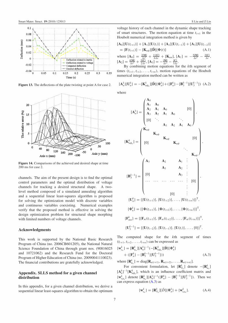
triangular function of time, the iteration history is shown infigure 10. The optimum time-dependent control voltage ofeach channel and the optimum voltage channel distribution areplotted in figures 11 and 12. The voltage variations illustratedin figure 11 are almost the same as those defined by thedesired time functions except in the vicinities of the non-smooth points. The time-dependent deflections at point A areillustrated in figure 13, from which we can see that the desireddynamic shape is achieved with high precision. Figure 14shows the relative error between the actuated and desired shapeat 200 ms, which shows the desired twisting shape is matchedwell at the specified moment.

6. Conclusion

This paper presents an investigation into constrained dynamicshape control of a composite plate with PZT actuators. ThePZT actuators are controlled by limited numbers of voltage

6

Smart Mater. Struct. 19 (2010) 125013 S Liu and Z Lin

Figure 13. The deflections of the plate twisting at point A for case 2.

Figure 14. Comparisons of the achieved and desired shape at time200 ms for case 2.

channels. The aim of the present design is to find the optimalcontrol parameters and the optimal distribution of voltagechannels for tracking a desired structural shape. A two-level method composed of a simulated annealing algorithmand a sequential linear least-squares algorithm is proposedfor solving the optimization model with discrete variablesand continuous variables coexisting. Numerical examplesverify that the proposed method is effective in solving thedesign optimization problem for structural shape morphingwith limited numbers of voltage channels.

Acknowledgments

This work is supported by the National Basic ResearchProgram of China (no. 2006CB601205), the National NaturalScience Foundation of China through grant nos. (90816025and 10721062) and the Research Fund for the DoctoralProgram of Higher Education of China (no. 20090041110023).The financial contributions are gratefully acknowledged.

Appendix. SLLS method for a given channeldistribution

In this appendix, for a given channel distribution, we derive asequential linear least-squares algorithm to obtain the optimum

voltage history of each channel in the dynamic shape trackingof smart structures. The motion equation at time ti+1 in theHoubolt numerical integration method is given by

[A0]{U(ti+1)} + [A1]{U(ti)} + [A2]{U(ti−1)} + [A3]{U(ti−2)}= {F(ti+1)} − [Kuφ][D]{Φ(t)} (A.1)

where [A0] = 2[M]�t2 + 11[C]

6�t + [Kuu], [A1] = − 5[M]�t2 − 3[C]

�t ,[A2] = 4[M]

�t2 + 3[C]2�t , [A3] = −[M]

�t2 − [C]3�t .

By combining motion equations for the kth segment oftimes (ti+1, ti+2, . . . , ti+n), motion equations of the Houboltnumerical integration method can be written as

[Akn]{Uk

n} = −[Kkuφn

][D]{Φkn}+({Fk

n}−[Bk−13 ]{Uk−1

3 }) (A.2)

where

[Akn] =

⎛⎜⎜⎜⎜⎜⎜⎝

A0

A1 A0

A2 A1 A0 [0]A3 A2 A1 A0

[0] . . .. . .

A3 A2 A1 A0

⎞⎟⎟⎟⎟⎟⎟⎠

,

[Kkuφn

] =

⎛⎜⎜⎜⎜⎜⎜⎝

Kuφ

Kuφ

Kuφ [0][0] Kuφ

. . .

Kuφ

⎞⎟⎟⎟⎟⎟⎟⎠

,

[Bk−13 ] =

⎛⎜⎜⎜⎜⎜⎜⎜⎜⎜⎜⎝

A3 A2 A1...

A3 A2...

[0] A3...

· · · · · · · · · · · · · · · ... [0]...

[0] ...

⎞⎟⎟⎟⎟⎟⎟⎟⎟⎟⎟⎠

,

{Ukn} = {{U(ti+1)}, {U(ti+2)}, . . . , {U(ti+n)}}T,

{Φkn} = {{Φ(ti+1)}, {Φ(ti+2)}, . . . , {Φ(ti+n)}}T,

{Fkmn} = {{Fm(ti+1)}, {Fm(ti+2)}, . . . , {Fm(ti+n)}}T,

{Uk−13 } = {{U(ti−2)}, {U(ti−1)}, {U(ti)}, . . . , {0}}T.

The computed shape for the kth segment of times(ti+1, ti+2, . . . , ti+n) can be expressed as

{wkcn

} = [Rkun

][Akn]−1(−[Kk

uφn][D]{Φk

n}+ ({Fk

n} − [Bk−13 ]{Uk−1

3 })) (A.3)

where [Rkun

] = diag[Ru(i+1), Ru(i+2), . . . , Ru(i+n)].For convenient formulation, let [Rk

Vn] denote −[Rk

un]

[Akn]−1[Kk

uφn], which is an influence coefficient matrix and

{wkcρn

} denote [Rkun

][Akn]−1({Fk

n} − [Bk−13 ]{Uk−1

3 }). Then wecan express equation (A.3) as

{wkcn

} = [RkVn

][D]{Φkn} + {wk

cρn}. (A.4)

7

Smart Mater. Struct. 19 (2010) 125013 S Liu and Z Lin

The desired shapes at times (ti+1, ti+2, . . . , ti+n) can be writtenas

{wkdn} = {{wd(ti+1)}, {wd(ti+2)}, . . . , {wd(ti+n)}}T. (A.5)

The error function over a time period can be defined by

E({�kn}) = {{wk

cn} − {wk

dn}}T{{wk

cn} − {wk

dn}}

= {[RkVn

][D]{Φkn} + {wk

cρn} − {wk

dn}}T{[Rk

Vn][D]{Φk

n}+ {wk

cρn} − {wk

dn}}. (A.6)

The optimal voltages are then obtained by imposing

∂ E

∂{Φkn}

= 0 (A.7)

which gives

[D]T[RkVn

]T[RkVn

][D]{Φkn} = [Rk

Vn]T({wk

dn} − {wk

cρn}). (A.8)

References

[1] Alkhatib R and Golnaraghi M F 2003 Active structuralvibration control: a review Shock Vib. Dig. 35 367–83

[2] Chopra I 2002 Review of state of art of smart structures andintegrated systems AIAA J. 40 2145–87

[3] Lin M, Qing X, Kumar A and Beard S J 2001 Smart layer andsmart suitcase for structural health monitoring applicationsProc. SPIE 4332 98–106

[4] Hurlebausa H and Gaul L 2006 Smart structure dynamicsMech. Syst. Signal Process. 20 255–81

[5] Irschiik H 2002 A review on static and dynamic shape controlof structures by piezoelectric actuation Eng. Struct. 24 5–11

[6] Frecker M I 2003 Recent advances in optimization of smartstructures J. Intell. Mater. Syst. Struct. 14 207–16

[7] Koconis D B, Kollar L P and Springer G S 1994 Shape controlof composite plates and shells with embedded actuators II:desired shape specified J. Compos. Mater. 28 262–85

[8] Hsu C Y, Lin C C and Gaul L 1997 Shape control of compositeplates by bonded actuators with high performanceconfiguration J. Reinf. Plast. Compos. 16 1692–710

[9] Chee C, Tong L and Steven G 2000 A buildup voltagedistribution (BVD) algorithm for shape control of smartplate structures Comput. Mech. 26 115–28

[10] Liew K M, He X Q and Ray T 2004 On the use ofcomputational intelligence in the optimal shape control offunctionally graded smart plates Comput. Methods Appl.Mech. Eng. 193 4475–92

[11] Chen W, Wang D and Li M 2004 Static shape controlemploying displacement–stress dual criteria Smart Mater.Struct. 13 468–72

[12] Merkhujee A and Joshi S 2002 Piezoelectric sensors andactuators spatial design for shape control of piezolaminatedplates AIAA J. 40 1204–10

[13] Shaik Dawood M S I, Iannucci L and Greenhalgh E S 2008Three-dimensional static shape control analysis of compositeplates using distributed piezoelectric actuators Smart Mater.Struct. 17 025002

[14] Liu S, Tong L and Lin Z 2008 Simultaneous optimization ofcontrol parameters and configurations of PZT actuators formorphing structural shapes Finite Elem. Anal. Des.44 417–24

[15] Forster E and Livne E 2000 Integrated design optimization ofstrain actuated structures for dynamic shape controlAIAA-2000-1366

[16] Luo Q and Tong L 2006 A sequential linear least squarealgorithm for tracking dynamic shapes of smart structuresInt. J. Numer. Methods Eng. 67 66–88

[17] Luo Q and Tong L 2007 A segment based sequential leastsquares algorithm with optimum energy control for trackingthe dynamic shapes of smart structures Smart Mater. Struct.16 1517–26

[18] Youssef H, Sait S M and Adiche H 2001 Evolutionaryalgorithms, simulated annealing and tabu search: acomparative study Eng. Appl. Artif. Intell. 14 167–81

[19] Kirkpatrick S, Gelatt C D Jr and Vecchi M P 1983 Optimizationby simulated annealing Science 220 671–80

[20] Wang L 2001 Intelligent Optimization Algorithms withApplications (Beijing: Tsinghua University Press)

[21] Luo Q and Tong L 2006 High precision shape control of platesusing orthotropic piezoelectric actuators Finite Elem. Anal.Des. 42 1009–20

8