093904

Hindawi Publishing CorporationJournal of Control Science and EngineeringVolume 2007, Article ID 93904, 12 pagesdoi:10.1155/2007/93904

Research ArticleThe Best Achievable H2 Tracking Performancesfor SIMO Feedback Control Systems

Shinji Hara,1 Toni Bakhtiar,1 and Masaaki Kanno2

1 Department of Information Physics and Computing, The University of Tokyo, 7-3-1 Hongo, , Bunkyo-Ku ,Tokyo 113-8656, Japan

2 Japan Science and Technology Agency, 4-1-8 Honcho, Kawaguchi-Shi , Saitama 332-0012, Japan

Received 20 August 2006; Revised 10 January 2007; Accepted 12 April 2007

Recommended by Sigurd Skogestad

This paper is concerned with the inherent H2 tracking performance limitation of single-input and multiple-output (SIMO) lineartime-invariant (LTI) feedback control systems. The performance is measured by the tracking error between a step reference inputand the plant output with additional penalty on control input. We employ the plant augmentation strategy, which enables usto derive analytical closed-form expressions of the best achievable performance not only for discrete-time system, but also forcontinuous-time system by exploiting the delta domain version of the expressions.

Copyright © 2007 Shinji Hara et al. This is an open access article distributed under the Creative Commons Attribution License,which permits unrestricted use, distribution, and reproduction in any medium, provided the original work is properly cited.

1. INTRODUCTION

Problems concerning the fundamental performance limita-tions and tradeoff in feedback control systems have been in-tensively studied for decades motivated by the work of Bodeon logarithmic sensitivity integral [1]. There are two main re-search directions in the area. First direction lies in the exten-sions of Bode’s integral theorem to assess design constraintsand performance limitations via logarithmic type integrals(see, e.g., [2, 3]). Second direction focuses on the formula-tions of optimal control problems to quantify and charac-terize the fundamental performance limits in terms of plantparameters or properties.

Research in the latter direction relates to the plant/con-troller design integration, where the main attention is not todesign a robust or optimal controller but to design a plantwhich is easily controllable in practice. Therefore, study oncontrol performance limitations achievable by feedback con-trol has been paid much attention in the recent years as seenin a special issue of the IEEE Transactions on Automatic Con-trol in August 2003 and books by Seron et al. [4] and by Sko-gestad and Postletwaite [5].

Optimal tracking and regulation problems are two im-portant research topics which follow the second direction. Inthe former problem, the tracking ability is measured by theminimal tracking error between output and reference inputand is optimized over all possible stabilizing controllers. In

the latter problem, the control performance is measured bythe control input energy against impulsive disturbance input.

In particular, the H2 tracking performance limitationachievable by feedback control has been intensively in-vestigated, which has led to some complete results forsingle-input and single-output (SISO) continuous/discrete-time/sampled-data systems. Beyond the SISO case, existingresults on the optimal tracking performance problem includethe single-input and multiple-output (SIMO) [6, 7] andmultiple-input and multiple-output (MIMO) [8–10] cases.Results on the H2 energy regulation problem are availablefor continuous-time systems [11] and discrete-time systems[12]. A recent result which is formulated in the state spaceapproach and in both of the H2 and H∞ optimal controlframeworks can be found in [13]. It is known that the energyregulation problem relates closely to the problem of feedbackstabilization over signal-to-noise ratio constrained channels[14, 15].

In general, the existing results demonstrate in a clearmanner how the control performance level may be limitedby plant unstable poles and nonminimum phase zeros, andadditionally the directional aspects of such poles and zeros inthe case of a multivariable system.

This paper focuses on the H2 optimal tracking problemswith control input penalty for possibly unstable, nonmini-mum phase, SIMO LTI plants. The tracking performance ismeasured by the tracking error between the measurement

2 Journal of Control Science and Engineering

output and a step reference input with additional penalty oncontrol input. We note that none of the results for the SIMOor MIMO cases [6, 7, 9, 10] except one in [8] are practicallyuseful, since problems without control input constraint wereonly treated. Also [8] only considers the marginally stablecase. Moreover, the result in [9] is only valid for the MIMOright invertible case, where the number of inputs is greaterthan or equal to that of outputs. In other words, the resultcannot be applied to the SIMO case.

The problem formulation employed here is more realisticthan the problem without penalty on the control input, sincethe controller cannot produce an input beyond the capabil-ity of the actuator in practice. The treatment of the SIMOcase is also of practical significance, since in such a case, theplant to be controlled has only one actuator with two ormore sensors, which commonly appears in real control ap-plications to get better control performance by putting ex-tra sensors. The classes of feedback systems investigated herecover continuous-time and discrete-time systems and thusare fairly wide. We will provide comprehensive results of theanalytical closed-form expressions on the performance limi-tations by a unified approach (delta operator).

The main contribution of the present paper is to deriveanalytical closed-form expressions of the H2 optimal track-ing performance under control input penalty for SIMO LTIdiscrete-time systems. The idea of the derivation is to im-plement the well-known plant augmentation strategy, whichenables us to apply directly the result of the problem with-out control input penalty [6]. Corresponding expressions forcontinuous-time systems are derived by reformulating theproblem in terms of the delta operator [16]. Then, paralleldiscussions with the continuous-time case can be carried outfor the discrete-time case, where we strengthen the expres-sion for unstable plants presented in [7].

In general, our results show that the plant gain as wellas the plant’s nonminimum phase zeros and unstable polesimpose inevitable limitation on the tracking performance,and they are confirmed by a numerical example. We alsoapply the continuous-time results to an inverted pendulumsystem and provide the closed-form expression of the bestachievable tracking performances in terms of plant param-eters. This enables us to discuss the selection of the optimalpendulum length which gives the smallest possible value oftracking performance without solving the Riccati equationor the LMI problem corresponding to the H2 optimal con-trol problem.

The remainder of this paper is organized as follows. InSection 2, we describe the problem formulation includingthe description of the standard unity feedback control systemand a brief explanation about the plant augmentation strat-egy. Section 3 provides analytical closed-form expressions ofthe optimal performance in the discrete-time case. Section 4is devoted to the continuous-time results, where we apply theresults to an inverted pendulum system to show the effective-ness of our result for the plant design. We conclude the paperin Section 5 with remarks on the sampled-data feedback case.

The notation used throughout this paper is fairly stan-dard. We denote the real set by R and the complex set by C.

K Pr

−e u y

Figure 1: Unity feedback control system.

For any z ∈ C, its complex conjugate is denoted by z. Forany vector v we will use vT , vH , and ‖v‖ as its transpose, con-jugate transpose, and Euclidean norm, respectively. For anymatrix A ∈ Cm×n, we denote its conjugate transpose by AH

and its column space by R[A]. Several subsets in the com-plex plane are defined as follows: C− := {s ∈ C : Re s < 0},C+ := {s ∈ C : Re s > 0}, C+ := {s ∈ C : Re s ≥ 0},D := {z ∈ C : |z| < 1}, Dc := {z ∈ C : |z| ≥ 1},D

c:= {z ∈ C : |z| > 1}. We denote by RH∞ the set of

all rational matrix functions which are bounded and analyticin Dc. We define by x(z) the Z-transform of sequence x(k).The cardinality of a set S is denoted by #S.

2. PROBLEM FORMULATION

2.1. Feedback control systems

We consider the LTI unity feedback control system depictedin Figure 1, where P denotes a SIMO LTI plant to be con-trolled and K is a stabilizing controller. The plant P can bewritten as

P = (

P1,P2, . . . ,Pm)T

, (1)

where Pi (i = 1, . . . ,m) are scalar transfer functions. The sig-nals r ∈ Rm, u ∈ R, y ∈ Rm, and e := r − y ∈ Rm arethe reference input, the control input, the measurement out-put, and the error signals, respectively. Hereafter, it will beassumed that all the vectors and matrices involved in the se-quel have compatible dimensions.

The plant rational transfer function P admits right andleft coprime factorizations

P = NM−1 = ˜M−1Ñ , (2)

where N ,M, Ñ , ˜M ∈ RH∞, and there exist X ,Y , ˜X , ˜Y ∈RH∞ that satisfy the double Bezout identity

(

˜X − ˜Y

− Ñ ˜M

)(

M YN X

)

= I. (3)

The set of all stabilizing controllers K is then characterizedby the Youla parameterization

K := {

K : K = (Y −MQ)(NQ− X)−1

= (Q Ñ − ˜X)−1( ˜Y −Q˜M); Q ∈ RH∞}

.(4)

We only focus on the discrete-time case in the remainderof this section and the next section, while the continuous-time case will be discussed in Section 4.

A number η ∈ C is said to be a zero of P if Pi(η) = 0 holdsfor some i = 1, . . . ,m. In addition, if η lies in D

c, then η is

Shinji Hara et al. 3

said to be a nonminimum phase zero. The plant P is said to beminimum phase if it has no nonminimum phase zeros; oth-erwise, it is said to be nonminimum phase. A number λ ∈ Cis said to be a pole of P if P(λ) is unbounded. If λ lies in D

c,

then λ is an unstable pole of P. We say P is stable if it has nounstable poles; otherwise, it is unstable. An equivalent state-ment for pole λ is that ˜M(λ)w = 0 for some unitary vector w,and w is called a pole direction vector associated with λ. Fortechnical reasons, it is assumed that the plant does not havenonminimum phase zeros and unstable poles at the same lo-cation.

A transfer function Θ, not necessarily square, is called aninner if Θ is in RH∞ and Θ∼(z)Θ(z) = I for all z = e jθ .Here we define Θ∼(z) := ΘT(z−1). A transfer function Φ iscalled an outer if Φ is in RH∞ and has a right inverse whichis analytic in D

c. For P ∈ RH∞,

P(z) = Θ(z)Φ(z), (5)

where Θ is an inner and Φ is an outer, is called an inner-outerfactorization of P. We call Θ the inner factor and Φ the outerfactor.

2.2. H2 optimal tracking problem

The problem to be investigated in this paper is the standardH2 optimal tracking problem, where we consider a unit stepfunction r as the reference input signal defined by

r(k) =⎧

⎨

⎩

ν, k ≥ 0

0, k < 0, r(z) = zν

z − 1(6)

with ν = (ν1, ν2, . . . , νm)T is a constant vector of unit lengthand specifies the direction of the reference input. An exten-sion of this benchmark case can be undertaken by consider-ing other typical classes of reference signals such as real si-nusoids and ramp signals [10]. This result shows that non-minimum phase zeros and unstable poles maintain a signifi-cant role even in a more complex fashion and lead to a rathercomplicated expression of the optimal performance. Anotherextension may also dwell on the use of noncausal action fortracking such as preview control [17].

The performance index to be minimized in the presentpaper is given by

Jd :=∞∑

k=0

(∥

∥e(k)∥

∥

2+∣

∣uw(k)∣

∣

2), (7)

where uw is the weighted control input, that is, uw(k) =Z−1{W(z)u(z)}, with proper, stable, and minimum phaseweighting function W(z). Note that, if W = 0, the problemthen reduces to an H2 tracking error minimization problem(i.e., the H2 optimal tracking problem without control inputpenalty), which has been discussed in [6, 7].

It follows from the well-known Parseval’s identity that (7)can be further written as

Jd =∥

∥e(z)∥

∥

22 +

∣

∣uw(z)∣

∣

22

= ∥

∥So(z)r(z)∥

∥

22 +

∣

∣W(z)K(z)So(z)r(z)∣

∣

22,

(8)

where So := (I + PK)−1 is the output sensitivity function.Using (2)–(4), the optimal performance can then be repre-sented by

J∗d = infQ∈RH∞

∥

∥

∥

∥

∥

{[

WYX

]

−[

WMN

]

Q

}

˜Mr

∥

∥

∥

∥

∥

2

2

. (9)

We make the following standard assumptions to guaran-tee the finiteness of Jd.

Assumption 1. N(1) �= 0.

Assumption 2. For r(k) in (6), ν ∈ R[N(1)].

Assumption 3. P(z) has a pole at z = 1.

In order for Jd to be finite, it is obvious that the outputsensitivity function So must have a zero at z = 1 with inputzero direction ν, that is, So(1)ν = 0. The condition N(1) �= 0is then required to avoid any hidden pole-zero cancelationat z = 1 so that the open loop system has an integrator inthe discrete-time sense. The condition ν ∈ R[N(1)] requiresthat the input signal must enter from the direction lying inthe column space of N(1) and gives the condition of stepreference signal r so that a nonright invertible plant P maytrack. In order to make the steady state error zero, the open-loop transfer function PK must contain an integrator. Con-sequently, plant P must have an integrator instead of com-pensator K , which should have no integrator to maintain afinite control energy cost. Assumption 3 is thus necessary.

2.3. Plant augmentation

To solve the tracking error problem under control penalty,we adopt the well-known plant augmentation approach. Thiskey idea is initially implemented in solving the tracking per-formance problem in one of the authors’ conference papers[11].

An augmented plant Pa is defined as

Pa :=(

WP

)

, (10)

from which we obtain the corresponding step input signalra := (0, rT)T with direction νa := (0, νT)T and the trackingmeasure

Jda :=∞∑

k=0

∥

∥ea(k)∥

∥

2, (11)

where

ea :=(

0r

)

−(

uwy

)

. (12)

One of the key points addressed by this strategy is that thetracking measure does not explicitly include the control in-put penalty u.

Furthermore, the corresponding right and left coprimefactorizations of Pa are expressed as

Pa = NaM−1a = ˜M−1

a˜Na, (13)


where

Na =(

WMN

)

, Ma =M,

˜Ma =(

1 00 ˜M

)

, Ña =(

WÑ

)

,

(14)

and the corresponding double Bezout identity is written as⎛

⎝

˜Xa − ˜Ya

− Ña ˜Ma

⎞

⎠

(

Ma Ya

Na Xa

)

= I , (15)

where Ya = (0,Y), ˜Xa = ˜X , ˜Ya = (0, ˜Y), and

Xa =(

1 WY0 X

)

. (16)

With a free parameter Qa = (Q0,Q) ∈ RH∞, where Q0 is anew scalar free parameter, the optimal tracking performanceJ∗da can be expressed as

J∗da = infQa∈RH∞

∥

∥

(

Xa −NaQa)

˜Mara∥

∥

22, (17)

and subsequently, we have

J∗da = infQ∈RH∞

∥

∥

∥

∥

∥

{[

WYX

]

−[

WMN

]

Q

}

˜Mr

∥

∥

∥

∥

∥

2

2

. (18)

The expression of J∗da in (18) is exactly equivalent to that ofJ∗d in (9) for the original plant P, that is, J∗da = J∗d holds. Bytaking into account that there is no explicit penalty imposedon the control input for computing J∗da in (18), we can im-mediately follow the approach of the tracking error problemin [6] to derive the analytical closed-form expression of J∗d .

3. DISCRETE-TIME CASE

3.1. Closed-form expression

This section provides an analytical closed-form expression ofthe optimal tracking performance for the discrete-time case.The derivation is almost parallel to the continuous-time case[7, 11].

Note first that (17) can be expressed as

J∗d = infQa∈RH∞

∥

∥

∥

∥

[

I + Na(

˜Ya −Qa˜Ma)] νaz − 1

∥

∥

∥

∥

2

2. (19)

Write N = (N1, . . . ,Nm)T with Ni (i = 0, 1, . . . ,m) beingscalar transfer functions, and

Na =(

N0,N)T

, (20)

where N0 = WM. We denote by λk ∈ Dc(k = 1, . . . ,nλ) the

unstable poles of P(z) and by ηi j ∈ Dc

(i = 1, . . . ,m, j =1, . . . ,ni) the nonminimum phase zeros of Pi(z).

We further define the following index sets:

Jz := {

i : Ni(1) �= 0}

,

Jp := {

k : ˜M(

λk)

ν = 0}

,

Jpi := {

k : Ni(

λk) = 0

}

(i = 0, 1, . . . ,m).

(21)

Note that Jp contains the index of unstable poles whose di-rection is coincident with that of the step input signal r. Dueto the relation N = PM, Jpi contains the index of unstablepoles of P but not those of Pi. The index set Jpi will play akey role of strengthening the expression for unstable plantsin [7], where we explicitly identify the nonminimum phasezeros of N . To facilitate our derivation, we introduce the fol-lowing inner-outer factorization of Na(z):

Na(z) = Θ(z)Φ(z), (22)

where Θ is an inner factor and Φ is an outer factor.

Theorem 1. Suppose that the SIMO plant P(z) given in (1)has unstable poles λk (k = 1, . . . ,nλ) and Pi(z) has nonmini-mum phase zeros ηi j (i = 1, . . . ,m, j = 1, . . . ,ni). Then, underAssumptions 1–3, the optimal tracking performance J∗d is givenby

J∗d = Jds + Jdu, (23)

where

Jds = Jds1 + Jds2 (24)

with

Jds1 :=∑

i∈Jzν2i

ni∑

j=1

∣

∣ηi j∣

∣

2 − 1∣

∣ηi j − 1∣

∣

2 ,

Jds2 := 12π

∑

i∈Jzν2i

∫ π

0log

[∣

∣Pi(1)∣

∣

2

∥

∥P(1)∥

∥

2 ×∥

∥P(

e jθ)∥

∥

2+∣

∣W(

e jθ)∣

∣

2

∣

∣Pi(

e jθ)∣

∣

2

]

× dθ

1− cos θ,

Jdu = Jdu1 + Jdu2

(25)

with

Jdu1 :=∑

i∈Jzν2i

∑

k∈Jpi

∣

∣λk∣

∣

2 − 1∣

∣λk − 1∣

∣

2 ,

Jdu2 :=∑

k,�∈Jp

(∣

∣λk∣

∣

2 − 1)(∣

∣λ�∣

∣

2 − 1)

hkh�(

λk − 1)(

λ� − 1)(

λkλ� − 1)

× (

1−Θ∼

(

λk)

Θ(1))(

1−Θ∼

(

λ�)

Θ(1))

,

hk :=

⎧

⎪

⎪

⎨

⎪

⎪

⎩

1; #Jp = 1,∏

�∈Jp , � �=k

λk − λ�1− λ�λk

; #Jp ≥ 2.

(26)

Proof. See the appendix for the proof.

Theorem 1 reveals that the optimal performance intracking a step reference signal is explicitly characterized bythe plant’s nonminimum phase zeros ηi j and unstable polesλk, the plant direction [18] which is mostly determined by


the plant gain, and the reference input direction ν. Further-more, the problem of minimizing the tracking error undercontrol input penalty generally provides additional limits im-posed by W , which appears in the logarithmic term in Jds2and the inner factor Θ in Jdu2.

If we set W = 0 then we can easily obtain the nonpenaltyresult [6]. If the plant is marginally stable, we can see J∗d = Jds(or, Jdu = 0). In this theorem we also provide a stronger ex-pression than that in [7] by examining explicitly additionaleffects caused by unstable poles λk in Jcu1. We defer the dis-cussion of this part until the end of Section 4.2, while statingfirst a number of remarks and corollaries of Theorem 1.

We may also derive the optimal controller within thisapproach. For (marginally) stable case, for instance, we canmake the term (A.9) in the appendix zero by selecting theoptimal free parameter Q∗a as

Q∗a (z) =[

Θ∼(1)Φ(z)

+ ˜Ya(z)]

˜M−1a (z). (27)

The expression of the optimal controller can then be ob-tained by following the Youla parameterization (4). For un-stable case, we need additional effort to simplify the expres-sion of Q∗a .

3.2. Remarks and corollaries

We here note that Jds1 and Jdu1 in Theorem 1 reflect the ef-fects contributed by nonminimum phase zeros and unsta-ble poles. Such zeros or poles close to the unit circle mayor may not have a significant effect depending on the in-put direction νi and those farther outside the unit circleprovide less effect. An interesting fact may also be drawnconcerning with the zero at infinity. Immediately we have(|ηi j|2 − 1)/|ηi j − 1|2 → 1 as ηi j → ∞, which reveals thatin discrete-time system one zero at infinity contribute onepenalty to the performance level. Therefore without loss ofgenerality the effect of time delays can be treated as a num-ber of zeros at infinity, instead of directly handled as a timedelay system as in [8, 10], which provides a consistent result.The second term Jds2 concerns the effect due to the changesin the plant direction with frequency, (see [7, 18]).

Now we make a couple of remarks on the last term Jdu2,in particular, on the existence of the inner factor Θ(z).

(1) The expression in the theorem is complete for SIMOmarginally stable plants in the sense that the bestachievable tracking performance with control inputpenalty is characterized by nonminimum phase ze-ros and the gain of the plant without using any in-ner outer factors or solving any Riccati equation. (SeeCorollary 1 for the SISO case).

(2) The expression for the general unstable case is notcomplete in that it includes an inner factor Θ(z) in thelast term Jdu2. We can only obtain a closed-form ex-pression of Θ(z) for the SISO without control inputpenalty case. (see Corollary 2).

(3) However, fortunately, there exists a special case wherethe term Jdu2 caused by unstable poles is zero even ifthe plant is unstable. (see Corollary 3).

(4) We can also show that Jdu = Jdu1 + Jdu2 is zero whenthe sets of all unstable poles of Pi(z) (i = 1, . . . ,m) arecompletely the same as seen in Corollary 4. The caseoften happens for practical applications where we haveonly one actuator but we may add one or more extrasensors. The extra sensor can dramatically improve thetracking performance for unstable and nonminimumphase plants as seen in the example of an inverted pen-dulum in Section 4.3.

We now consider four specific cases for illustrating theimplication of Theorem 1. The first case is the simplest case,where we consider a (marginally) stable scalar system.

Corollary 1. Suppose that the plant P(z) is SISO marginallystable and has nonminimum phase zeros ηi (i = 1, . . . ,nη).Under Assumptions 1 and 3, one has

J∗d =nη∑

i=1

∣

∣ηi∣

∣

2−1∣

∣ηi−1∣

∣

2 +1

2π

∫ π

0

log[

1+∣

∣W(

e jθ)∣

∣

2/∣∣P

(

e jθ)∣

∣

2]

1−cos θdθ.

(28)

By Corollary 1, the effect of constant wighting functionW can be understood easily, where a bigger W makes thecontrol effort more costly and thus worsen the performancelevel. The performance can also be constrained by minimumphase zeros close to the unit circle, since in the vicinity ofsuch zeros |P(e jθ)| is rather small. In addition, in the low-frequency range such zeros may have more negative effectdue to the terms 1/(1 − cos θ). In some limited and sim-ple cases, we can obtain the closed expression of the integralterm. For example, if P(z) = (z − η)/z(z − 1) (0 < η < 1)and W = 1, then

J∗d = 1 +η −

√

η2 + 2η + 5 + 1

2(η − 1), (29)

where the first term of the right-hand side is caused by a zeroat infinity and the second one corresponds to the integralterm. We can readily see from the second term that the mini-mum phase zero η also affects the performance limit and thatit tends to infinity as η goes to one.

The second corollary is for the SISO without control in-put penalty case, that is, W(z) = 0. Suppose the plant hasnonminimum phase zeros ηi (i = 1, . . . ,nη). Then the innerfactor in (22) can, without loss of generality, be fixed as

Θ(z) =nη∏

i=1

z − ηi1− ηiz

, (30)

from which we get Θ(1) = 1. Let φ(z) := Θ∼(z)Θ(1), that is,

φ(z) =nη∏

i=1

1− ηiz

z − ηi. (31)

Then the achievable performance for SISO without controlinput penalty case can be stated as follows.


Corollary 2. Consider the nonpenalty case, that is, W(z) = 0,for the SISO plant P(z) which has nonminimum phase zeros ηi(i = 1, . . . ,nη) and unstable poles λk (k = 1, . . . ,nλ). Then, onehas

J∗d =nη∑

i=1

∣

∣ηi∣

∣

2 − 1∣

∣ηi − 1∣

∣

2 +∑

k,�∈Jp

(∣

∣λk∣

∣

2 − 1)(∣

∣λ�∣

∣

2 − 1)

hkh�(

λk − 1)(

λ� − 1)(

λkλ� − 1)

× (

1− φ(

λk))(

1− φ(

λ�))

.(32)

The third corollary is for a special class of SIMO unstablesystems, where the tracking performance limit is explicitlygiven in terms of plant characteristics.

Corollary 3. Let the SIMO plant P satisfy P(1) =[P1(1), 0, . . . , 0]T , and let the input signal r be given by (6)with ν = (1, 0, . . . , 0)T . Suppose that P1(z) is (marginally) sta-ble and has nonminimum phase zeros η1 j ( j = 1, . . . ,n1) andP has unstable poles λk (k = 1, . . . ,nλ). Then, one has

J∗d =n1∑

j=1

∣

∣η1 j∣

∣

2 − 1∣

∣η1 j − 1∣

∣

2 +∑

k∈Jp1

∣

∣λk∣

∣

2 − 1∣

∣λk − 1∣

∣

2

+1

2π

∫ π

0

log[(∥

∥P(e jθ)∥

∥

2+∣

∣W(

e jθ)∣

∣

2)/∣∣P1

(

e jθ)∣

∣

2]

1− cos θdθ.

(33)

Proof. Since ν = (1, 0, . . . , 0)T , only the nonminimum phasezeros and the plant gain of P1(z) give effects. The unstablepoles of P(z) contributed by Pi(z) (i ≥ 2), if any, will not giveeffects through Jdu2, that is, Jdu2 = 0, since the pole directionsdo not coincide with that of the input signal, that is ˜M(λk)ν �=0, but through Jdu1 as the nonminimum phase zeros of N1(z).

The last corollary deals with SIMO plant P(z), in whichthe set of unstable poles of Pi(z) (i = 1, . . . ,m) are completelythe same.

Corollary 4. Consider the SIMO plant P(z) given in (1).Suppose that Pi(z) has nonminimum phase zeros ηi j (i =1, . . . ,m, j = 1, . . . ,ni) and has unstable poles λk (k =1, . . . ,nλ) for all i = 1, . . . ,m, that is, the set of unstable polesof Pi(z) are the same. Then, one has

J∗d = Jds1 + Jds2. (34)

Proof. If the set of unstable poles of Pi(z) (i = 1, . . . ,m) arecompletely the same, then it is not difficult to verify that Jpiis empty for i = 1, . . . ,m. Note that Jp0 may not be empty,but this will not give any effect since the first element of νais zero. Furthermore, we know that Jp is also empty for the

case, since ˜M(λk)ν �= 0 for all k = 1, . . . ,nλ. These two factsmake Jdu1 = 0 and Jdu2 = 0. Hence, Jdu = 0.

k = 1

k = 2

k = 4

0 0.5 1 1.5

W

6

6.5

7

7.5

J∗ d

Figure 2: J∗d with respect to k and W .

3.3. Numerical example

Consider a single-input two-output discrete-time plant P(z)given by

P(z) =[

P1(z)P2(z)

]

=

⎡

⎢

⎢

⎢

⎣

z − η

(z − 1)(1− 2z)k(z − 1)z(z − λ)

⎤

⎥

⎥

⎥

⎦

, (35)

where |λ| > 1 and k > 0. Thus, P1(z) is (marginally) stableand has nonminimum phase zeros at z = ∞ and z = η pro-vided |η| > 1, and P2(z) has one nonminimum phase zero atz = ∞ and one unstable pole at z = λ.

We can easily see that coprime factors of P(z) can be writ-ten as

N(z) =

⎡

⎢

⎢

⎢

⎣

(z − η)(z − λ)z(1− 2z)(1− λz)

k(z − 1)2

z2(1− λz)

⎤

⎥

⎥

⎥

⎦

, M(z) = (z − 1)(z − λ)z(1− λz)

,

˜M(z) =

⎡

⎢

⎢

⎣

z − 1z

0

0z − λ

1− λz

⎤

⎥

⎥

⎦

, ˜N(z) =

⎡

⎢

⎢

⎢

⎣

z − η

z(1− 2z)k(z − 1)z(1− λz)

⎤

⎥

⎥

⎥

⎦

.

(36)

We choose ν = (1, 0)T ∈ R[N(1)], which gives ˜M(λ)ν �=0. Therefore, this example is in the case of Corollary 3. Wecalculate the optimal tracking performance J∗d based on theexpression in the corollary. Note that the first element ofN(z), N1(z), includes a nonminimum phase zero at z = λwhich is an unstable pole of P2(s) in addition to the originalzeros at z = ∞ and z = η. This extra zero in N1(z) yields thesecond term of J∗d . For example, Figure 2 depicts the optimaltracking performance for η = 2 and λ = 3 with respect to


W = 1W = 2W = 3

0.6 0.7 0.8 0.9 1 1.1 1.2 1.3 1.4 1.5

η

0

5

10

15

20

25

30

35

40

45

50

J∗ d

Figure 3: J∗d with respect to η and W .

k = {1, 2, 4} and W from 0 to 1.5. In this case, the optimalperformance is given by

J∗d = 6 +1

2π

∫ π

0

log[

1 +(∣

∣P2(

e jθ)∣

∣

2+ W2

)/∣

∣P1(e jθ)∣

∣

2]

1− cos θdθ,

(37)

where the first term of the right-hand side is calculated as

6 = limη∞→∞

η2∞ − 1(

η∞ − 1)2 +

η2 − 1(

η − 1)2 +

λ2 − 1(

λ− 1)2 (38)

with η = 2 and λ = 3.We can see from Figure 2 that bigger k increases the gain

of P2(z) while larger W makes the control effort more expen-sive. Furthermore, Figure 3 plots the achievable performancefor k = 1, W = {1, 2, 3}, and λ = 3 when η varies from 0.6to 1.5. It is shown that the performance tends to infinity as ηtends to 1 from either side. A minimum phase zero close to 1makes |P1(e jθ)| small, thus rendering the integral term large,and a nonminimum phase zero close to 1 blows the first termup.

4. CONTINUOUS-TIME CASE

4.1. Approach using δ-operator

This section is devoted to the continuous-time case and wederive an analytical closed-form expression of the minimalvalue of the performance index

Jc :=∫∞

0

(∥

∥e(t)∥

∥

2+∣

∣uw(t)∣

∣

2)dt (39)

for the continuous-time plant P(s), where uw(t) =L−1{W(s)u(s)}. To this end, we invoke the delta domain

expression by reformulating the discrete-time problem interms of the delta operator [16], and we show that we canreadily derive the continuous-time counterpart based on thediscrete-time result obtained in the previous section.

For any sequence x(k), k = 1, 2, . . . , the delta operator δis defined by

δx(k) = x(k + 1)− x(k)T

, (40)

where T > 0 is the sampling time. By taking the Z-transformof the above equation we obtain

δx(z) = z − 1T

x(z). (41)

Hence, we obtain the relationship between the Z-transformvariable z and the delta operator δ as

δ = z − 1T

or z = Tδ + 1. (42)

Furthermore, for any sequence x(k) we define its delta trans-form by

D{

x(k)} = xT(δ) := T

∞∑

k=0

x(k)(Tδ + 1)−k, (43)

or equivalently, xT(δ) = Tx(z)|z=Tδ+1.The optimal performance J∗c is then recovered by letting

the sampling time T approach zero in the following perfor-mance index:

JT := T∞∑

k=0

(∥

∥e(k)∥

∥

2+∣

∣uw(k)∣

∣

2), (44)

where uw(k) = D−1{W(δ)uT(δ)}. We here omit the deriva-tion process since it can be done in a straightforward man-ner. For instance, it is immediate to derive the delta domaincounterparts of Lemmas 1 and 2 in the appendix. The com-plete derivation is given in [19].

The delta domain expression, however, helps us to under-stand the dynamics of the solution with respect to the sam-pling time T . In addition, making T tend to zero will recoverthe continuous-time results in [7], which is rewritten in thefollowing section.

4.2. Closed-form expression

For the finiteness of Jc we impose the following assumptionsfor P(s) with coprime factorizations (2).

Assumption 4. N(0) �= 0.

Assumption 5. ν ∈ R[N(0)].

Assumption 6. P(s) has a pole at s = 0.

We denote by pk ∈ C+ (k = 1, . . . ,np) the unstable polesof P(s) and by zi j ∈ C+ (i = 1, . . . ,m, j = 1, . . . ,ni) the


nonminimum phase zeros of Pi(s). We further introduce thefollowing index sets:

Iz := {

i : Ni(0) �= 0}

,

Ip := {

k : ˜M(

pk)

ν = 0}

,

Ipi := {

k : Ni(

pk) = 0

}

(i = 0, 1, . . . ,m).

(45)

Define an inner-outer factorization of Na(s) such that

Na(s) = Θ(s)Φ(s), (46)

and subsequently define Θ∼(s) := ΘT(−s).

Theorem 2. Suppose that the SIMO plant P(s) given in (1)has unstable poles pk (k = 1, . . . ,np) and Pi(s) has nonmini-mum phase zeros zi j (i = 1, . . . ,m, j = 1, . . . ,ni). Then, underAssumptions 4–6, the optimal tracking performance J∗c is givenby

J∗c = Jcs + Jcu, (47)

where

Jcs = Jcs1 + Jcs2 (48)

with

Jcs1 :=∑

i∈Izν2i

ni∑

j=1

2 Re zi j∣

∣zi j∣

∣

2 ,

Jcs2 := 1π

∑

i∈Izν2i

∫∞

0log

[∣

∣Pi(0)∣

∣

2

∥

∥P(0)∥

∥

2 ×∥

∥P( jω)∥

∥

2+∣

∣W( jω)∣

∣

2

∣

∣Pi( jω)∣

∣

2

]

× dω

ω2,

Jcu = Jcu1 + Jcu2

(49)

with

Jcu1 :=∑

i∈Izν2i

∑

k∈Ipi

2 Re pk∣

∣pk∣

∣

2 ,

Jcu2 :=∑

k,�∈Ip

4 Re pk Re p�(

pk + p�)

pk p�σkσ�

× (

1−Θ∼

(

pk)

Θ(0))(

1−Θ∼

(

p�)

Θ(0))

,

σk :=

⎧

⎪

⎪

⎨

⎪

⎪

⎩

1; #Ip = 1,∏

�∈Ip ,� �=k

p� − pkp� + pk

; #Ip ≥ 2.

(50)

In the case of W = 0, that is, the problem without controlinput penalty, the expressions in Theorem 2 validate those in[7, Theorem 3.3] in a more explicit form. In the above the-orem we explicitly spell out the effect of the nonminimumphase zeros of N into two terms Jcs1 and Jcu1, while [7, Theo-rem 3.3] writes it out as a single term J∗s , the optimal perfor-mance with respect to the stable part of the plant Ps. In our

Mu

x

mg

θ

Figure 4: The inverted pendulum system.

version, Jcs1 accounts for the effects contributed by nonmini-mum phase zeros zi j (i ∈ Iz) of the plant P and Jcu1 identifiesthose affected by unstable poles pk (k ∈ Ipi). Then it is re-vealed that unstable poles may also deteriorate the achievableperformance in the same way as nonminimum phase zeros.This fact, however, is not elucidated in [7].

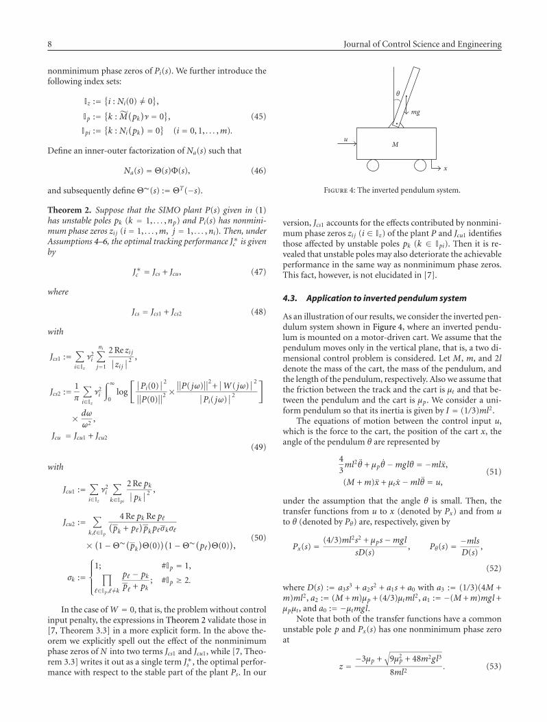
4.3. Application to inverted pendulum system

As an illustration of our results, we consider the inverted pen-dulum system shown in Figure 4, where an inverted pendu-lum is mounted on a motor-driven cart. We assume that thependulum moves only in the vertical plane, that is, a two di-mensional control problem is considered. Let M, m, and 2ldenote the mass of the cart, the mass of the pendulum, andthe length of the pendulum, respectively. Also we assume thatthe friction between the track and the cart is μt and that be-tween the pendulum and the cart is μp. We consider a uni-form pendulum so that its inertia is given by I = (1/3)ml2.

The equations of motion between the control input u,which is the force to the cart, the position of the cart x, theangle of the pendulum θ are represented by

43ml2θ + μpθ −mglθ = −mlx,

(M + m)x + μtx −mlθ = u,(51)

under the assumption that the angle θ is small. Then, thetransfer functions from u to x (denoted by Px) and from uto θ (denoted by Pθ) are, respectively, given by

Px(s) = (4/3)ml2s2 + μps−mgl

sD(s), Pθ(s) = −mls

D(s),

(52)

where D(s) := a3s3 + a2s2 + a1s + a0 with a3 := (1/3)(4M +m)ml2, a2 := (M +m)μp + (4/3)μtml2, a1 := −(M +m)mgl+μpμt, and a0 := −μtmgl.

Note that both of the transfer functions have a commonunstable pole p and Px(s) has one nonminimum phase zeroat

z =−3μp +

√

9μ2p + 48m2gl3

8ml2. (53)


Now we derive analytical closed-form expressions for thebest achievable tracking error performance J∗c for two differ-ent cases, namely, the SISO case (Case 1): P(s) = Px(s), andthe SITO case (Case 2): P(s) = [Px(s),Pθ(s)]T . We assumeW(s) = 1 for simplicity and define the following functions:

f1(ω) := ω2[(a0 − a2ω2)2

+(

a1ω− a3ω3)2]

,

f2(ω) := m2l2(

43lω2 + g

)2

+ μ2pω

2.(54)

Case 1. The control objective in this case is to stabilize thesystem by measuring the cart position x only. The optimaltracking performance is given by

J∗c1 = Jz +1π

∫∞

0log

[

1 +f1(ω)f2(ω)

]

dω

ω2

+2[

1−Θ∼(p)Θ(0)]2

p,

(55)

where p is the unstable pole of Px(s) and

Jz = 16ml2

−3μp +√

9μ2p + 48m2gl3

. (56)

Note that, in (55), Θ(s) is determined from the followinginner-outer factorization:

[

Mx(s)Nx(s)

]

= Θ(s)Φ(s), (57)

where Px(s) = Nx(s)Mx(s)−1.Figure 5 illustrates the situation in Case 1. Here we as-

sume that the ratio between the mass and the length of thependulum is constant, that is, m/l = 2.145π [kg/m] andM = 2 [kg]. We also assume that μt = 1/4 and μp = 1/3. Wecompute the optimal tracking performance for l from 1 to4 [m] by using (55), that is, Theorem 2. We can see from thefigure that the values of J∗c1 are fairly large which are caused bythe third term of J∗c1. Although the optimal length of the pen-dulum which gives the lowest possible value of J∗c1 is around2.8 [m], it is implied that the stabilization by a single sensorof the cart position is very hard in practice.

One of the reasonable practical solutions is to add an ex-tra sensor which measures the pendulum angle θ. Indeed, thecontinuous-time counterpart of Corollary 4 can be appliedto the case and a reasonable result can be obtained as seenbelow.

Case 2. We will control both the cart position x and the pen-dulum angle θ by measuring those two quantities. Note thatPθ(0) = 0, which leads to the step input direction ν = (1, 0)T .Thanks to the shared unstable pole in both Px(s) and Pθ(s),the optimal tracking error performance is simply representedby

J∗c2 = Jz +1π

∫∞

0log

[

1 +f1(ω) + m2l2ω4

f2(ω)

]

dω

ω2. (58)

The values of optimal costs J∗c2 for Case 2 are quite smallin comparison with J∗c1 as seen in Figure 6. The main reason

1 1.5 2 2.5 3 3.5 4

l (m)

0.9

0.95

1

1.05

1.1

1.15

1.2×105

J∗ c1

Figure 5: The optimal tracking performance of Case 1.

0 0.5 1 1.5 2

l (m)

3

3.5

4

4.5

5

5.5

6J∗ c2

Figure 6: The optimal tracking performance of Case 2.

is that the unstable pole p does not give any effect, that is,J∗cu = 0, since p is a common pole of Px(s) and Pθ(s), and itsdirection is not coincident with that of step input signal, thatis, ˜M(p)ν �= 0.

Although the expression (58) is rather complicated, itonly includes the plant parameters. Hence, we can directlysee the relation between the best achievable control perfor-mance and the plant parameters without solving the corre-sponding Riccati equation or the LMI problem. This is oneof the advantages of deriving the closed-form expression. Forexample, we can see that Jz is a monotone increasing func-tion of the length l, while the second term in (58) tends toinfinity when the length l goes to zero. These clearly indicatethat there exists an optimal length l which minimizes the H2

cost (58). In fact, Figure 6 shows that the best length of thependulum is about 0.2 [m] for this case.


r(t) e(t)

− Sek uk u(t) y(t)

Kd H Pc

Figure 7: Sampled-data feedback control system.

rk[1 0 . . . 0] −

rk ek uk yk0Kd

Ptyk

P f0

ek−

Figure 8: Approximation of the sampled-data feedback control sys-tem.

5. CONCLUSION

We have examined the H2 tracking performance problemfor SIMO LTI feedback control systems, where the trackingperformance is quantified by the error response with con-trol input penalty. We first provided analytical closed-formexpressions of the best achievable tracking performance fordiscrete-time systems by introducing the idea of plant aug-mentation. We have addressed several cases where we canhave complete solutions for the H2 performance limits. Wenext discussed the continuous-time case by exploiting thedelta domain expression based on the discrete-time resultand derived the continuous-time counterpart. We then ap-plied the result to an inverted pendulum system to confirmthe effectiveness of the closed-form expression in plant de-sign.

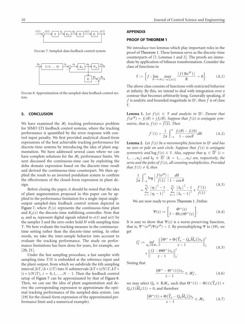
Before closing the paper, it should be noted that the ideaof plant augmentation proposed in this paper can be ap-plied to the performance limitation for a single-input single-output sampled-data feedback control system depicted inFigure 7, where Pc(s) represents the continuous-time plantand Kd(z) the discrete-time stabilizing controller. Note thatek and uk represent digital signals related to e(t) and u(t) bythe sampler S and the zero-order hold H with sampling timeT . We here evaluate the tracking measure in the continuous-time setting rather than the discrete-time setting. In otherwords, we take the inter-sample behavior into account toevaluate the tracking performance. The study on perfor-mance limitations has been done for years, for example, see[20, 21].

Under the fast sampling procedure, a fast sampler withsampling time T/N is embedded at the reference input andthe plant output, from which we subdivide the kth samplinginterval [kT , (k+1)T) into N subintervals [kT+(i/N)T , kT+(i + 1/N)T), i = 0, 1, . . . ,N − 1. Then the feedback controlsetup of Figure 7 can be approximated by that of Figure 8.Then, we can use the idea of plant augmentation and de-rive the corresponding expression to approximate the opti-mal tracking performance of the sampled-data system. (see[19] for the closed-form expression of the approximated per-formance limit and a numerical example).

APPENDIX

PROOF OF THEOREM 1

We introduce two lemmas which play important roles in theproof of Theorem 1. These lemmas serve as the discrete-timecounterparts of [7, Lemmas 1 and 2]. The proofs are imme-diate by application of bilinear transformation. Consider theclass of functions in

F :={

f : limR→∞

maxθ∈[−π/2,π/2]

∣

∣ f(

Re jθ )∣

∣

R= 0

}

. (A.1)

The above class consists of functions with restricted behaviorat infinity. By this, we intend to deal with integration over acontour that becomes arbitrarily long. Generally speaking, iff is analytic and bounded magnitude inDc, then f is of classF.

Lemma 1. Let f (z) ∈ F and analytic in Dc. Denote thatf (e jθ) = f1(θ) + j f2(θ). Suppose that f (z) is conjugate sym-metric, that is, f (z) = f (z). Then

f ′(1) = 12π

∫ π

−πf1(θ)− f1(0)

1− cos θdθ. (A.2)

Lemma 2. Let f (z) be a meromorphic function in Dc and hasno zero or pole on unit circle. Suppose that f (z) is conjugatesymmetric and log f (z) ∈ F. Also, suppose that ηi ∈ Dc

(i =1, . . . ,nη) and λk ∈ D

c(k = 1, . . . ,nλ) are, respectively, the

zeros and the poles of f (z), all counting multiplicities. Providedthat f (1) �= 0, then

12π

∫ π

−πlog

∣

∣

∣

∣

f (e jθ)f (1)

∣

∣

∣

∣

dθ

1− cos θ

=nη∑

i=1

∣

∣ηi∣

∣

2 − 1∣

∣ηi − 1∣

∣

2 −nλ∑

k=1

∣

∣λk∣

∣

2 − 1∣

∣λk − 1∣

∣

2 +f ′(1)f (1)

.

(A.3)

We are now ready to prove Theorem 1. Define

Ψ(z) :=[

Θ∼(z)I −Θ(z)Θ∼(z)

]

. (A.4)

It is easy to show that Ψ(z) is a norm-preserving function,that is, Ψ∼(e jθ)Ψ(e jθ) = I . By premultiplying Ψ to (19), weget

J∗d := infQa∈RH∞

∥

∥

∥

∥

[

Θ∼ + Φ(

˜Ya −Qa˜Ma)]

νaz − 1

∥

∥

∥

∥

2

2

+∥

∥

∥

∥

(

I −ΘΘ∼

)

νaz − 1

∥

∥

∥

∥

2

2.

(A.5)

Noting that(

Θ∼ −Θ∼(1))

νaz − 1

∈H⊥2 , (A.6)

we may select Qa ∈ RH∞ such that Θ∼(1) − Φ(1)( ˜Ya(1) +Qa(1)˜Ma(1)) = 0, and therefore

[

Θ∼(1) + Φ(

˜Ya −Qa˜Ma)]

νaz − 1

∈H2. (A.7)


As a result, we can write J∗d = J1 + J2, where

J1 :=∥

∥

∥

∥

(

Θ∼ −Θ∼(1))

νaz − 1

∥

∥

∥

∥

2

2+∥

∥

∥

∥

(

I −ΘΘ∼

)

νaz − 1

∥

∥

∥

∥

2

2, (A.8)

J2 := infQa∈RH∞

∥

∥

∥

∥

[

Θ∼(1) + Φ(

˜Ya −Qa˜Ma)]

νaz − 1

∥

∥

∥

∥

2

2. (A.9)

Next we will show that J1 = J∗ds1 + J∗ds2 + Jdu1 and J2 = Jdu2.A direct calculation leads to

J1 = − 12π

∫ π

−πRe

(

νHa Θ(

e jθ)

Θ∼(1)νa)− 1

1− cos θdθ. (A.10)

Let f (z) := νHa Θ(z)Θ∼(1)νa. Under Assumption 2, we ob-tain f (1) = 1. Applying Lemma 1 yields J1 = − f ′(1) =−νHa Θ(1)Θ∼(1)νa. Denote the inner factor Θ(z) in (22) asΘ(z) = [w0(z),w1(z), . . . ,wm(z)]T . According to Assump-tion 2, we may select νa = Θ(1) without loss of generality.Noting that the first element of νa is zero, we have

J1 = −m∑

i=0

wi(1)w′i (1) = −∑

i∈Jzν2iw′i (1)wi(1)

. (A.11)

Condition i ∈ Jz guarantees that wi(1) �= 0. Since wi(z) is anelement of the inner factor Θ(z), it has the same set of non-minimum phase zeros as Ni(z), which includes the set of un-stable poles of P but not those of Pi as well as the set of non-minimum phase zeros of Pi(z). Hence, by invoking Lemma 2,we have1

w′i (1)wi(1)

= −ni∑

j=1

∣

∣ηi j∣

∣

2 − 1∣

∣ηi j − 1∣

∣

2 −∑

k∈Jpi

∣

∣λk∣

∣

2 − 1∣

∣λk − 1∣

∣

2

+1

2π

∫ π

−πlog

∣

∣

∣

∣

wi(

e jθ)

wi(1)

∣

∣

∣

∣

dθ

1− cos θ.

(A.12)

Noting here that |wi(e jθ)| = |Pi(e jθ)|/‖Pa(e jθ)‖, we obtain

log∣

∣

∣

∣

wi(

e jθ)

wi(1)

∣

∣

∣

∣= −1

2log

[∣

∣Pi(1)∣

∣

2

∥

∥Pa(1)∥

∥

2

∥

∥Pa(

e jθ)∥

∥

2

∣

∣Pi(

e jθ)∣

∣

2

]

. (A.13)

We can see from Assumption 3 that |Pi(1)| and ‖P(1)‖ areinfinite but |W(1)| is finite, and therefore

∣

∣Pi(1)∣

∣

2

∥

∥Pa(1)∥

∥

2 =∣

∣Pi(1)∣

∣

2

∥

∥P(1)∥

∥

2+∣

∣W(1)∣

∣

2 =∣

∣Pi(1)∣

∣

2

∥

∥P(1)∥

∥

2 (A.14)

holds. Also note that

∥

∥Pa(

e jθ)∥

∥

2

∣

∣Pi(

e jθ)∣

∣

2 =∥

∥P(

e jθ)∥

∥

2+∣

∣W(

e jθ)∣

∣

2

∣

∣Pi(

e jθ)∣

∣

2 . (A.15)

1 The second term in the right-hand side is not explicitly examined in theexpression in [7].

This completes the proof of J1 = J∗ds1 +J∗ds2 +Jdu1. Next, by fac-torizing ˜Ma(z)νa = gm(z)h(z), where gm(z) is left invertiblein RH∞ and h(z) is defined by

h(z) =∏

k∈Jp

z − λk1− λkz

, (A.16)

we can show that J2 = Jdu2 by following the standard partialfraction expansion using in the proof of [7, Theorem 3.3].

REFERENCES

[1] H. W. Bode, Network Analysis and Feedback Amplifier Design,Van Nostrand, Princeton, NJ, USA, 1945.

[2] J. Chen, “Logarithmic integrals, interpolation bounds, andperformance limitations in MIMO feedback systems,” IEEETransactions on Automatic Control, vol. 45, no. 6, pp. 1098–1115, 2000.

[3] J. S. Freudenberg and D. P. Looze, “Right half plane poles andzeros and design tradeoffs in feedback systems,” IEEE Transac-tions on Automatic Control, vol. 30, no. 6, pp. 555–565, 1985.

[4] M. M. Seron, J. H. Braslavsky, and G. C. Goodwin, Fundamen-tal Limitations in Filtering and Control, Springer, London, UK,1997.

[5] S. Skogestad and I. Postletwaite, Multivariable Feedback Con-trol: Analysis and Design, John Wiley & Sons, Chichester, UK,2nd edition, 2005.

[6] T. Bakhtiar and S. Hara, “H2 control performance limitationsfor SIMO systems: a unified approach,” in Proceedings of the6th Asian Control Conference (ASCC ’06), pp. 555–563, Bali,Indonesia, July 2006.

[7] G. Chen, J. Chen, and R. Middleton, “Optimal tracking per-formance for SIMO systems,” IEEE Transactions on AutomaticControl, vol. 47, no. 10, pp. 1770–1775, 2002.

[8] J. Chen, S. Hara, and G. Chen, “Best tracking and regulationperformance under control energy constraint,” IEEE Transac-tions on Automatic Control, vol. 48, no. 8, pp. 1320–1336, 2003.

[9] J. Chen, L. Qiu, and O. Toker, “Limitations on maximal track-ing accuracy,” IEEE Transactions on Automatic Control, vol. 45,no. 2, pp. 326–331, 2000.

[10] O. Toker, J. Chen, and L. Qiu, “Tracking performance limita-tions in LTI multivariable discrete-time systems,” IEEE Trans-actions on Circuits and Systems I, vol. 49, no. 5, pp. 657–670,2002.

[11] S. Hara and C. Kogure, “Relationship between H2 control per-formance limits and RHP pole/zero locations,” in Proceedingsof the Society of Instrument and Control Engineers Annual Con-ference (SICE ’03), pp. 1242–1246, Fukui, Japan, August 2003.

[12] T. Bakhtiar and S. Hara, “H2 regulation performance limitsfor SIMO feedback control systems,” in Proceedings of the 17thInternational Symposium on Mathematical Theory of Networksand Systems (MTNS ’06), pp. 1966–1973, Kyoto, Japan, July2006.

[13] V. Kariwala, S. Skogestad, J. F. Forbes, and E. S. Meadows,“Achievable input performance of linear systems under feed-back control,” International Journal of Control, vol. 78, no. 16,pp. 1327–1341, 2005.

[14] J. H. Braslavsky, R. Middleton, and J. S. Freudenberg, “Feed-back stabilization over signal-to-noise ratio constrained chan-nels,” in Proceedings of the American Control Conference, vol. 6,pp. 4903–4908, Boston, Mass, USA, June-July 2004.


[15] R. Middleton, J. H. Braslavsky, and J. Freudenberg, “Stabiliza-tion of non-minimum phase plants over signal-to-noise ra-tio constrained channels,” in Proceedings of the 5th Asian Con-trol Conference (ASCC ’04), vol. 3, pp. 1914–1922, Melbourne,Australia, July 2004.

[16] R. Middleton and G. C. Goodwin, Digital Control and Estima-tion: A Unified Approach, Prentice-Hall, Englewood Cliffs, NJ,USA, 1990.

[17] J. Chen, Z. Ren, S. Hara, and L. Qiu, “Optimal tracking perfor-mance: preview control and exponential signals,” IEEE Trans-actions on Automatic Control, vol. 46, no. 10, pp. 1647–1653,2001.

[18] A. R. Woodyatt, M. M. Seron, J. S. Freudenberg, and R. Mid-dleton, “Cheap control tracking performance for non-right-invertible systems,” International Journal of Robust and Non-linear Control, vol. 12, no. 15, pp. 1253–1273, 2002.

[19] S. Hara and T. Bakhtiar, “H2 tracking performance limitationsfor SIMO feedback systems: a unified approach to control in-put penalty case,” Tech. Rep. METR2006-33, Department ofMathematical Informatics, The University of Tokyo, Tokyo,Japan, May 2006.

[20] J. Chen, S. Hara, L. Qui, and R. Middleton, “Best achievabletracking performance in sampled-data control systems,” inProceedings of the 41st IEEE Conference on Decision and Con-trol (CDC ’02), vol. 4, pp. 3889–3894, Las Vegas, Nev, USA,December 2002.

[21] J. S. Freudenberg, R. Middleton, and J. H. Braslavsky, “Inher-ent design limitations for linear sampled-data feedback sys-tems,” International Journal of Control, vol. 61, no. 6, pp. 1387–1421, 1995.

Submit your manuscripts athttp://www.hindawi.com

VLSI Design

Hindawi Publishing Corporationhttp://www.hindawi.com Volume 2014

International Journal of

RotatingMachinery


Hindawi Publishing Corporation http://www.hindawi.com

Journal ofEngineeringVolume 2014


Shock and Vibration


Mechanical Engineering

Advances in


Civil EngineeringAdvances in

Acoustics and VibrationAdvances in



Electrical and Computer Engineering

Journal of


Distributed Sensor Networks


The Scientific World JournalHindawi Publishing Corporation http://www.hindawi.com Volume 2014

SensorsJournal of


Modelling & Simulation in EngineeringHindawi Publishing Corporation http://www.hindawi.com Volume 2014


Active and Passive Electronic Components


Chemical EngineeringInternational Journal of

Control Scienceand Engineering

Journal of


Antennas andPropagation




Navigation and Observation


Advances inOptoElectronics

Hindawi Publishing Corporation http://www.hindawi.com

Volume 2014

RoboticsJournal of


093904

Documents

Transcript of 093904