09-Limited Dependent Variable Models
71
1 Limited Dependent Variable Models EMET 8002 Lecture 9 August 27, 2009
-
Upload
zhang-lucy -
Category
Documents
-
view
222 -
download
0
Transcript of 09-Limited Dependent Variable Models

8/3/2019 09-Limited Dependent Variable Models
http://slidepdf.com/reader/full/09-limited-dependent-variable-models 1/71
1
Limited Dependent VariableModels
EMET 8002
Lecture 9
August 27, 2009
8/3/2019 09-Limited Dependent Variable Models
http://slidepdf.com/reader/full/09-limited-dependent-variable-models 2/71
2
Limited Dependent Variables
A limited dependent variable is a dependentvariable whose range is restricted
For example: Any indicator variable such as whether or not a
household is poor (i.e., 0 or 1)
Test scores (generally bound by 0 and 100)
The number of children born to a woman is a non-negative integer

8/3/2019 09-Limited Dependent Variable Models
http://slidepdf.com/reader/full/09-limited-dependent-variable-models 3/71
3
Outline
Logit and probit models for binary dependentvariables
Tobit model for corner solutions

8/3/2019 09-Limited Dependent Variable Models
http://slidepdf.com/reader/full/09-limited-dependent-variable-models 4/71
4
Why do we care?
Let’s start with a review of the linear probabilitymodel to examine some of its shortcomings
The model is given by:
where
0 1 1 ...k k
y x x u β β β = + + + +
( ) ( ) 0 1 11| | ...k k
P y E y x x β β β = = = + + +x x

8/3/2019 09-Limited Dependent Variable Models
http://slidepdf.com/reader/full/09-limited-dependent-variable-models 5/71
5
Linear Probability Model
There will be three undesirable features of this model:
1.
The error term will not be homoskedastic. This violatesassumption LMR.4. Our OLS estimates will still be unbiased,but the standard errors are incorrect. Nonetheless, it is
easy to adjust for heteroskedasticity of unknown form.
2.
We can get predictions that are either greater than 1 orless than 0!
3.
The independent variables cannot be linearly related to thedependent variable for all possible values.
8/3/2019 09-Limited Dependent Variable Models
http://slidepdf.com/reader/full/09-limited-dependent-variable-models 6/71
6
Linear Probability Model
Example
Let’s look at how being in the labour force isinfluenced by various determinants:
Husband’s earnings
Years of education
Previous labour market experience
Age
Number of children less than 6 years old
Number of children between 6 and 18 years of age
8/3/2019 09-Limited Dependent Variable Models
http://slidepdf.com/reader/full/09-limited-dependent-variable-models 7/71
7
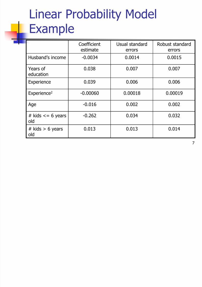
Linear Probability Model
ExampleCoefficientestimate
Usual standarderrors
Robust standarderrors
Husband’s income -0.0034 0.0014 0.0015
Years of education
0.038 0.007 0.007
Experience 0.039 0.006 0.006
Experience2 -0.00060 0.00018 0.00019
Age -0.016 0.002 0.002
# kids <= 6 yearsold
-0.262 0.034 0.032
# kids > 6 yearsold 0.013 0.013 0.014

8/3/2019 09-Limited Dependent Variable Models
http://slidepdf.com/reader/full/09-limited-dependent-variable-models 8/71
8
Linear Probability Model
Example
Using standard errors that are robust to unknownheteroskedasticity is simple and does notsubstantially change the reported standard errors
Interpreting the coefficients:
All else equal, an extra year of education increases theprobability of participating in the labour force by 0.038(3.8%)
All else equal, an additional child 6 years of age or lessdecreases the probability of working by 0.262
8/3/2019 09-Limited Dependent Variable Models
http://slidepdf.com/reader/full/09-limited-dependent-variable-models 9/71
9
Linear Probability Model
Example Predicted probabilities:
Sometimes we obtain predicted probabilities that are outsideof the range [0,1]. In this sample, 33 of the 753observations produce predicted probabilities outside of [0,1].
For example, consider the following observation: Husband’s earnings = 17.8
Years of education = 17
Previous labour market experience = 15
Age = 32
Number of children less than 6 years old = 0
Number of children between 6 and 18 years of age = 1
The predicted probability is 1.13!!
8/3/2019 09-Limited Dependent Variable Models
http://slidepdf.com/reader/full/09-limited-dependent-variable-models 10/71
10
Linear Probability Model
Example
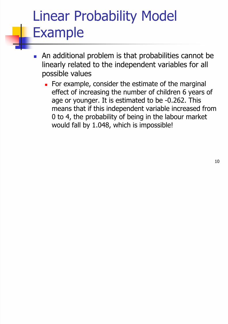
An additional problem is that probabilities cannot belinearly related to the independent variables for allpossible values
For example, consider the estimate of the marginaleffect of increasing the number of children 6 years of age or younger. It is estimated to be -0.262. Thismeans that if this independent variable increased from
0 to 4, the probability of being in the labour marketwould fall by 1.048, which is impossible!
8/3/2019 09-Limited Dependent Variable Models
http://slidepdf.com/reader/full/09-limited-dependent-variable-models 11/71
11
Linear Probability Model
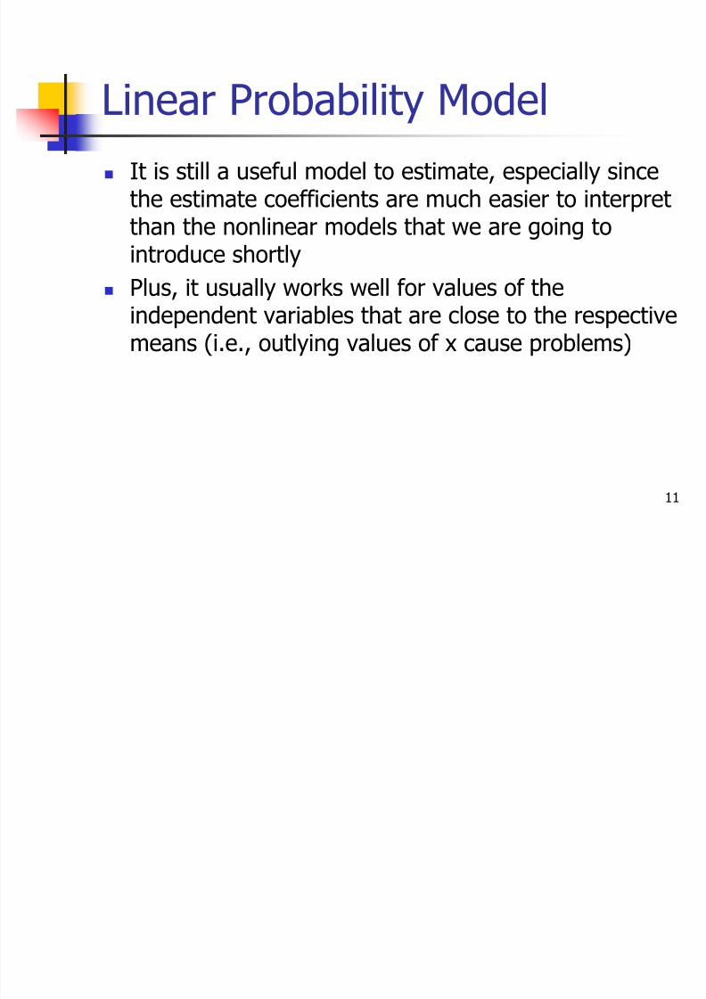
It is still a useful model to estimate, especially sincethe estimate coefficients are much easier to interpretthan the nonlinear models that we are going tointroduce shortly
Plus, it usually works well for values of theindependent variables that are close to the respectivemeans (i.e., outlying values of x cause problems)

8/3/2019 09-Limited Dependent Variable Models
http://slidepdf.com/reader/full/09-limited-dependent-variable-models 12/71
12
Limited Dependent Variables
Models
In this lecture we’re going to cover estimationtechniques that will better address the nature of thedependent variable
Logit & Probit
Tobit
8/3/2019 09-Limited Dependent Variable Models
http://slidepdf.com/reader/full/09-limited-dependent-variable-models 13/71
13
Logit and Probit Models for
Binary Response
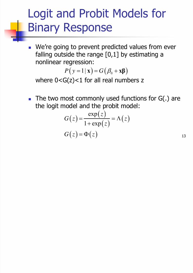
We’re going to prevent predicted values from everfalling outside the range [0,1] by estimating anonlinear regression:
where 0<G(z)<1 for all real numbers z
The two most commonly used functions for G(.) arethe logit model and the probit model:
( ) ( )01|P y G β = = +x xβ
( )( )
( )
( )
( ) ( )
exp
1 exp
zG z z
zG z z
= = Λ
+= Φ
8/3/2019 09-Limited Dependent Variable Models
http://slidepdf.com/reader/full/09-limited-dependent-variable-models 14/71
14
Logit and Probit Models for
Binary Response
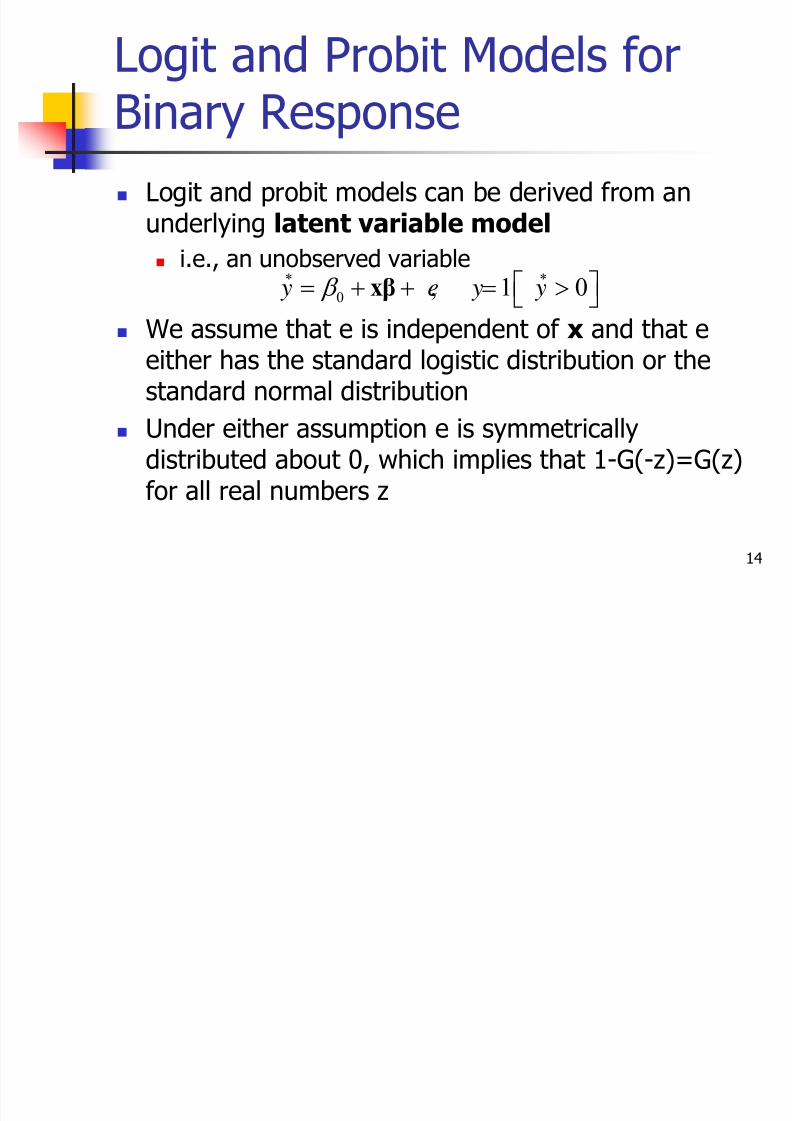
Logit and probit models can be derived from anunderlying latent variable model
i.e., an unobserved variable
We assume that e is independent of x and that eeither has the standard logistic distribution or thestandard normal distribution
Under either assumption e is symmetricallydistributed about 0, which implies that 1-G(-z)=G(z)for all real numbers z
* *
0 , 1 0 y e y y β ⎡ ⎤= + + = >⎣ ⎦xβ

8/3/2019 09-Limited Dependent Variable Models
http://slidepdf.com/reader/full/09-limited-dependent-variable-models 15/71
15
Logit and Probit Models for
Binary Response
We can now derive the response probability for y:( ) ( )( )
( )( )( )
( )
*
0
0
0
0
1| 0 |
0 |
|
1
P y P y
P e
P e
G
G
β
β
β
β
= = >
= + + >
= > − +
⎡ ⎤= − − +⎣ ⎦
= +
x x
xβ x
xβ x
xβ
xβ
8/3/2019 09-Limited Dependent Variable Models
http://slidepdf.com/reader/full/09-limited-dependent-variable-models 16/71
16
Logit and Probit Models for
Binary Response In most applications of binary response models our main
interest is to explain the effects of the x’s on the responseprobability P(y=1|x)
The latent variable interpretation tends to give the impression
that we are interested in the effects of the x’s on y* For probit and logit models, the direction of the effect of the x’s
on E(y*|x) and E(y|x)=P(y=1|x) are the same
In most applications however, the latent variable does not have
a well-defined unit of measurement which limits itsinterpretation. Nonetheless, in some examples this is a veryuseful tool for thinking about the problem.

8/3/2019 09-Limited Dependent Variable Models
http://slidepdf.com/reader/full/09-limited-dependent-variable-models 17/71
17
Logit and Probit Models for
Binary Response
The sign of the coefficients will tell us the direction of the partial effect of x j on P(y=1|x)
However, unlike the linear probability model, themagnitudes of the coefficients are not especiallyuseful
If x j is a roughly continuous variable, its partial effectis given by: ( ) ( )
j
j
p dG z
x dz
β ∂
=
∂
x

8/3/2019 09-Limited Dependent Variable Models
http://slidepdf.com/reader/full/09-limited-dependent-variable-models 18/71
18
Logit and Probit Models for
Binary Response In the linear probability model the derivative of G was simply 1,
since G(z)=z in the linear probability model.
In other words, we can move from this nonlinear functionback to the linear model by simply assuming G(z)=z.
For both the logit and the probit models g(z)=dG(z)/dz isalways positive (since G is the cumulative distribution function,g is the probability density function). Thus, the sign of β j is the
same as the sign of the partial effect.
The magnitude of the partial effect is influenced by the entirevector of x’s
8/3/2019 09-Limited Dependent Variable Models
http://slidepdf.com/reader/full/09-limited-dependent-variable-models 19/71
19
Logit and Probit Models for
Binary Response
Nonetheless, the relative effect of any twocontinuous explanatory variables do not depend on x
The ratio of the partial effects for x j and xh is β j /βh,which does not depend on x

8/3/2019 09-Limited Dependent Variable Models
http://slidepdf.com/reader/full/09-limited-dependent-variable-models 20/71
20
Logit and Probit Models for
Binary Response Suppose x1 is a discrete variable, its partial effect of going from
c to c+1 is given by:
Again, this effect depends on x
Note, however, that the sign of β1 is enough to know whetherthe discrete variable has a positive or negative effect
This is because G() is strictly increasing
( )( )
( )
0 1 2 2
0 1 2 2
1 ...
...
k k
k k
G c x x
G c x x
β β β β
β β β β
+ + + + + −
+ + + +
8/3/2019 09-Limited Dependent Variable Models
http://slidepdf.com/reader/full/09-limited-dependent-variable-models 21/71
21
Logit and Probit Models for
Binary Response
We use Maximum Likelihood Estimation, whichalready takes into consideration theheteroskedasticity inherent in the model
Assume that we have a random sample of size n
To obtain the maximum likelihood estimator,conditional on the explanatory variables, we need thedensity of yi given xi
( ) ( ) ( )
1
| ; 1 , 0,1
y y
i i i f y G G y
−
⎡ ⎤ ⎡ ⎤= − =⎣ ⎦ ⎣ ⎦x
βx
βx
β

8/3/2019 09-Limited Dependent Variable Models
http://slidepdf.com/reader/full/09-limited-dependent-variable-models 22/71
22
Logit and Probit Models for
Binary Response
When y=1: f(y| xi:β)=G( x
iβ)
When y=0: f(y| xi:β)=1-G( xiβ)
The log-likelihood function for observation i isgiven by:
The log-likelihood for a sample of size n is obtainedby summing this expression over all observations
( ) ( ) ( ) ( )log 1 log 1i i i i i
l y G y G⎡ ⎤ ⎡ ⎤= + − −⎣ ⎦ ⎣ ⎦β x β x β
( ) ( )1
n
i
i
L l
=
= ∑β β

8/3/2019 09-Limited Dependent Variable Models
http://slidepdf.com/reader/full/09-limited-dependent-variable-models 23/71
23
Logit and Probit Models for
Binary Response The MLE of β maximizes this log-likelihood
If G is the standard logit cdf, then we get the logitestimator
If G is the standard normal cdf, then we get the
probit estimator
Under general conditions, the MLE is:
Consistent Asymptotically normal
Asymptotically efficient
8/3/2019 09-Limited Dependent Variable Models
http://slidepdf.com/reader/full/09-limited-dependent-variable-models 24/71
24
Inference in Probit and Logit Models
Standard regression software, such as Stata, willautomatically report asymptotic standard errors forthe coefficients
This means we can construct (asymptotic) t-tests forstatistical significance in the usual way:
( )ˆ ˆ j j jt se β β =

8/3/2019 09-Limited Dependent Variable Models
http://slidepdf.com/reader/full/09-limited-dependent-variable-models 25/71
25
Logit
and Probit
Models for Binary
Response: Testing Multiple Hypotheses
We can also test for multiple exclusion restrictions(i.e., two or more regression parameters are equal to0)
There are two options commonly used:
A Wald test
A likelihood ratio test
8/3/2019 09-Limited Dependent Variable Models
http://slidepdf.com/reader/full/09-limited-dependent-variable-models 26/71
26
Logit
and Probit
Models for Binary
Response: Testing Multiple Hypotheses
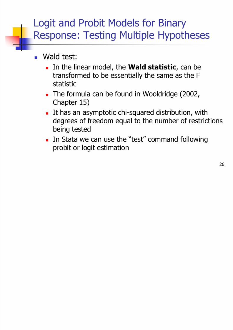
Wald test:
In the linear model, the Wald statistic, can betransformed to be essentially the same as the Fstatistic
The formula can be found in Wooldridge (2002,Chapter 15)
It has an asymptotic chi-squared distribution, with
degrees of freedom equal to the number of restrictionsbeing tested
In Stata we can use the “test” command followingprobit or logit estimation
8/3/2019 09-Limited Dependent Variable Models
http://slidepdf.com/reader/full/09-limited-dependent-variable-models 27/71
27
Logit
and Probit
Models for Binary
Response: Testing Multiple Hypotheses
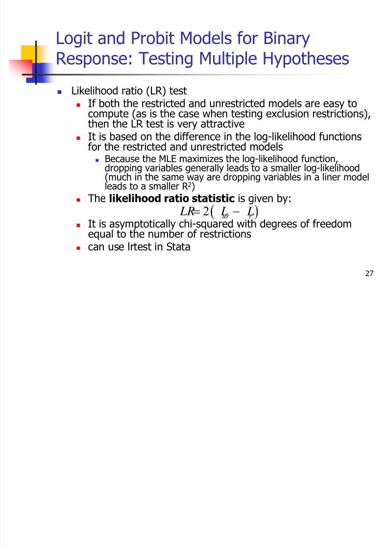
Likelihood ratio (LR) test If both the restricted and unrestricted models are easy to
compute (as is the case when testing exclusion restrictions),then the LR test is very attractive
It is based on the difference in the log-likelihood functions
for the restricted and unrestricted models Because the MLE maximizes the log-likelihood function,
dropping variables generally leads to a smaller log-likelihood(much in the same way are dropping variables in a liner modelleads to a smaller R 2)
The likelihood ratio statistic is given by:
It is asymptotically chi-squared with degrees of freedomequal to the number of restrictions
can use lrtest in Stata
( )2 ur r LR L L= −

8/3/2019 09-Limited Dependent Variable Models
http://slidepdf.com/reader/full/09-limited-dependent-variable-models 28/71
28
Logit and Probit Models for BinaryResponse: Interpreting Probit
and Logit
Estimates
Recall that unlike the linear probability model, theestimated coefficients from Probit or Logit estimationdo not tell us the magnitude of the partial effect of achange in an independent variable on the predicted
probability
This depends not just on the coefficient estimates,
but also on the values of all the independentvariables and the coefficients
8/3/2019 09-Limited Dependent Variable Models
http://slidepdf.com/reader/full/09-limited-dependent-variable-models 29/71
29
Logit and Probit Models for BinaryResponse: Interpreting Probit
and Logit
Estimates
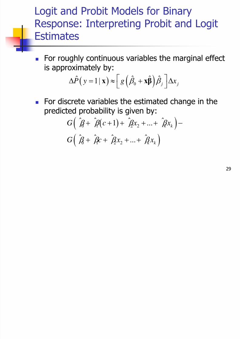
For roughly continuous variables the marginal effectis approximately by:
For discrete variables the estimated change in thepredicted probability is given by:
( ) ( )0ˆ ˆ ˆˆ 1|
j jP y g x β β ⎡ ⎤Δ = ≈ + Δ
⎣ ⎦x xβ
( )( )( )
0 1 2 2
0 1 2 2
ˆ ̂ ˆ ˆ1 ...
ˆ ˆ ˆ ˆ...
k k
k k
G c x x
G c x x
β β β β
β β β β
+ + + + + −+ + + +

8/3/2019 09-Limited Dependent Variable Models
http://slidepdf.com/reader/full/09-limited-dependent-variable-models 30/71
30
Logit and Probit Models for BinaryResponse: Interpreting Probit
and Logit
Estimates
Thus, we need to pick “interesting” value of x atwhich to evaluate the partial effects Often the sample averages are used. Thus, we obtain
the partial effect at the average (PEA)
We could also use lower or upper quartiles, forexample, to see how the partial effects change assome elements of x get large or small
If xk is a binary variable, then it often makes sense touse a value of 0 or 1 in the partial effect equation,
rather than the average value of xk

8/3/2019 09-Limited Dependent Variable Models
http://slidepdf.com/reader/full/09-limited-dependent-variable-models 31/71
31
Logit and Probit Models for BinaryResponse: Interpreting Probit
and Logit
Estimates
An alternative approach is to calculate the averagepartial effect (APE)
For a continuous explanatory variable, x j, the APE is:
The two scale factors (at the mean for PEA andaveraged over the sample for the APE) differ sincethe first uses a nonlinear function of the average and
the second uses the average of a nonlinear function
( ) ( )1 1
0 0
1 1
ˆ ˆ ̂ ˆ ˆ ̂n n
i j i j
i i
n g n g β β β β − −
= =
⎡ ⎤ ⎡ ⎤+ = +⎣ ⎦ ⎣ ⎦∑ ∑x β x β

8/3/2019 09-Limited Dependent Variable Models
http://slidepdf.com/reader/full/09-limited-dependent-variable-models 32/71
32
Example 17.1: Married Women’s
Labour Force Participation
We are going to use the data in MROZ.RAW toestimate a labour force participation for women usinglogit and probit estimation.
The explanatory variables are nwifeinc, educ, exper,
exper2, age, kidslt6, kidsge6
probit inlf nwifeinc educ exper expersq age kidslt6kidsge6
8/3/2019 09-Limited Dependent Variable Models
http://slidepdf.com/reader/full/09-limited-dependent-variable-models 33/71
33
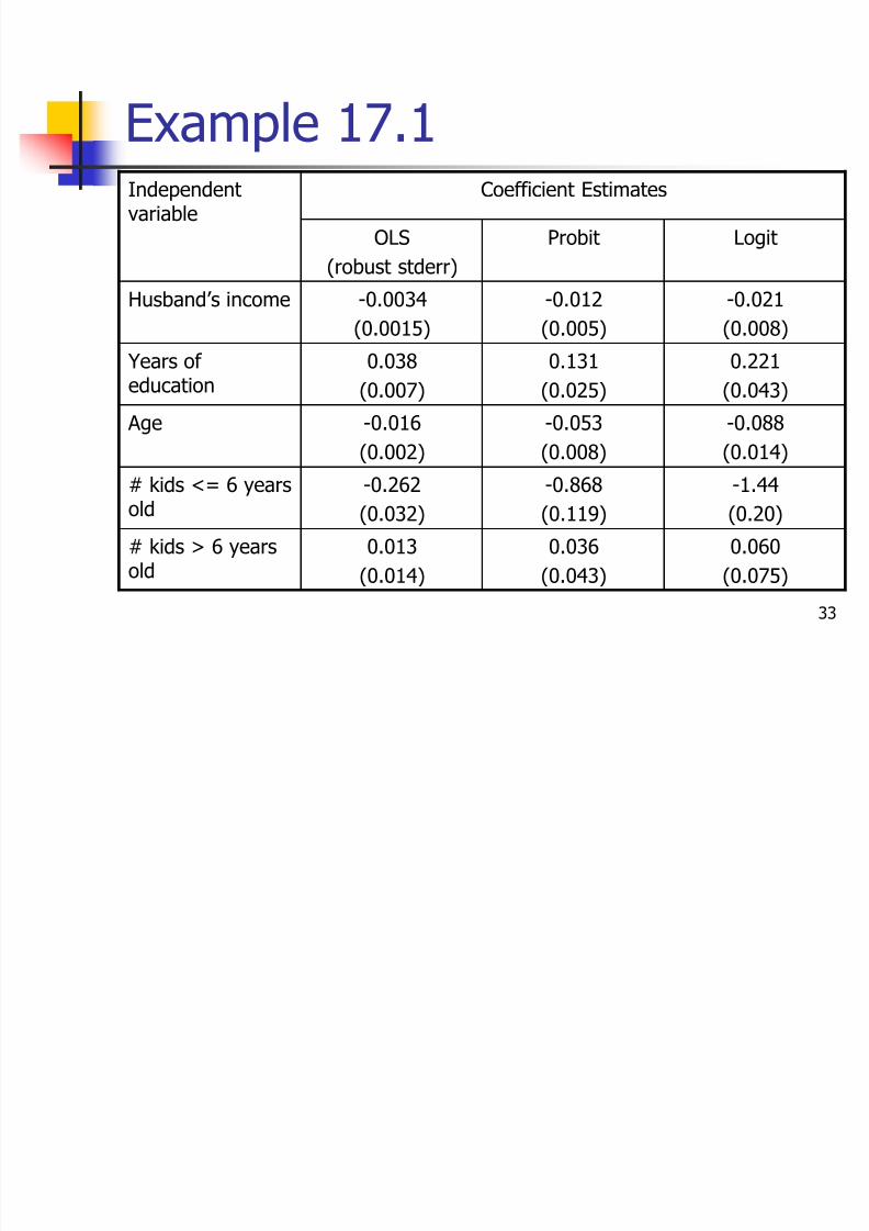
Example 17.1Independentvariable
Coefficient Estimates
OLS
(robust stderr)
Probit Logit
Husband’s income -0.0034
(0.0015)
-0.012
(0.005)
-0.021
(0.008)
Years of education
0.038
(0.007)
0.131
(0.025)
0.221
(0.043)
Age -0.016
(0.002)
-0.053
(0.008)
-0.088
(0.014)# kids <= 6 yearsold
-0.262
(0.032)
-0.868
(0.119)
-1.44
(0.20)
# kids > 6 years
old
0.013
(0.014)
0.036
(0.043)
0.060
(0.075)

8/3/2019 09-Limited Dependent Variable Models
http://slidepdf.com/reader/full/09-limited-dependent-variable-models 34/71
34
Example 17.1
True or false:
The Probit and Logit model estimates suggest that thelinear probability model was underestimating thenegative impact of having young children on the
probability of women participating in the labour force.
8/3/2019 09-Limited Dependent Variable Models
http://slidepdf.com/reader/full/09-limited-dependent-variable-models 35/71
35
Example 17.1
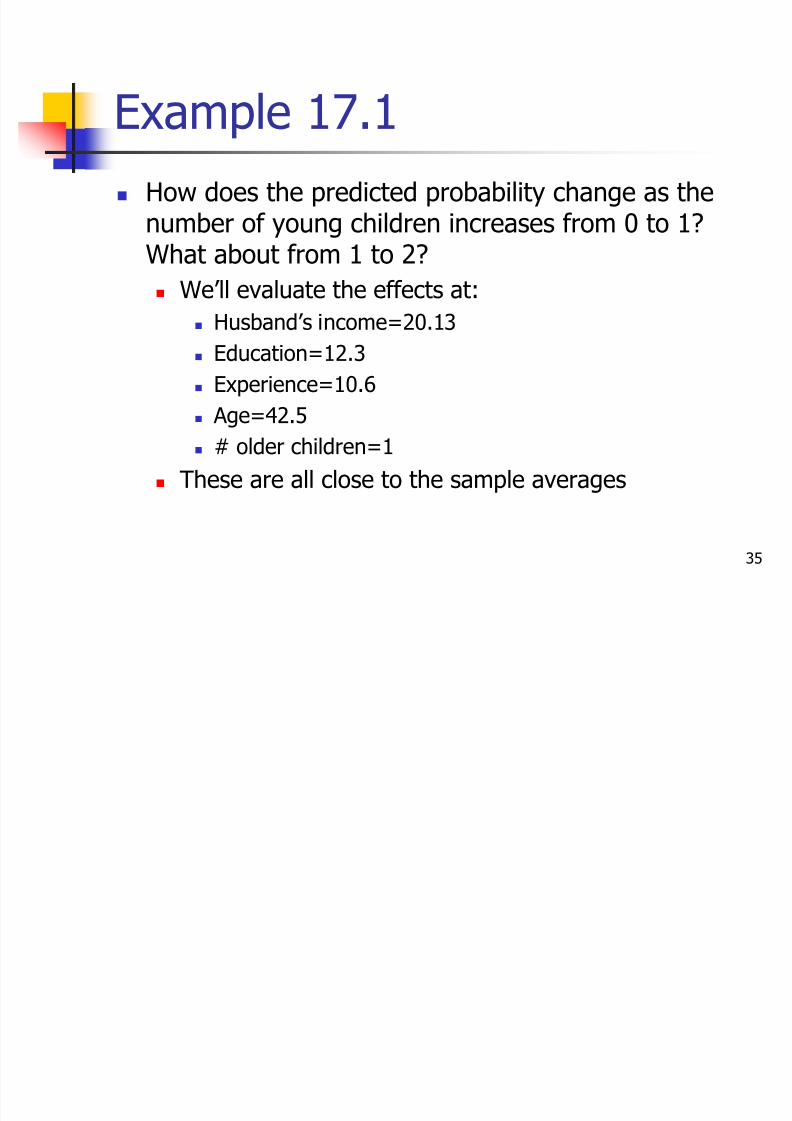
How does the predicted probability change as thenumber of young children increases from 0 to 1?What about from 1 to 2?
We’ll evaluate the effects at:
Husband’s income=20.13
Education=12.3
Experience=10.6
Age=42.5 # older children=1
These are all close to the sample averages
8/3/2019 09-Limited Dependent Variable Models
http://slidepdf.com/reader/full/09-limited-dependent-variable-models 36/71
36
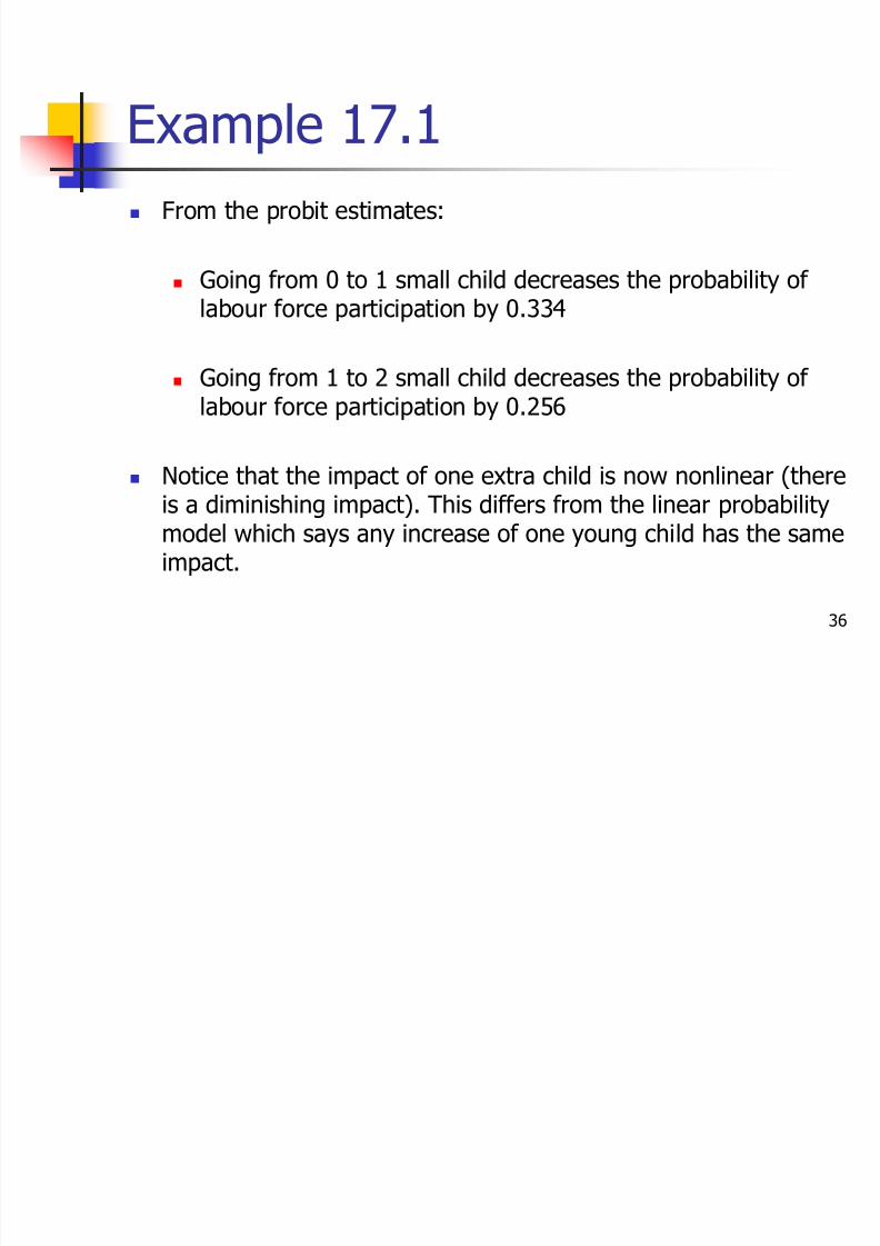
Example 17.1 From the probit estimates:
Going from 0 to 1 small child decreases the probability of labour force participation by 0.334
Going from 1 to 2 small child decreases the probability of labour force participation by 0.256
Notice that the impact of one extra child is now nonlinear (thereis a diminishing impact). This differs from the linear probabilitymodel which says any increase of one young child has the same
impact.

8/3/2019 09-Limited Dependent Variable Models
http://slidepdf.com/reader/full/09-limited-dependent-variable-models 37/71
37
Logit
and Probit
Models for Binary
Response
Similar to linear models, we have to be concerned with
endogenous explanatory variables. We don’t have time to coverthis so see Wooldridge (2002, Chapter 15) for a discussion
We need to be concerned with heteroskedasticity in probit andlogit models. If var(e| x) depends on x then the responseprobability no longer has the form G(β0+β x) implying that moregeneral estimation techniques are required
The linear probability can be applied to panel data, typically
estimated using fixed effects Logit and probit models with unobserved effects are difficult
to estimate and interpret (see Wooldridge (2002, Chapter15))

8/3/2019 09-Limited Dependent Variable Models
http://slidepdf.com/reader/full/09-limited-dependent-variable-models 38/71
38
The Tobit Model for Corner
Solution Responses
Often in economics we observes variables for which 0(or some other fixed number) is in an optimaloutcome for some units of observations, but a rangeof positive outcomes prevail for other observations
For example:
Number of hours worked annually
Trade flows
Hours spent on the internet Grade on a test (may be grouped at both 0 and 100)

8/3/2019 09-Limited Dependent Variable Models
http://slidepdf.com/reader/full/09-limited-dependent-variable-models 39/71
39
The Tobit Model for Corner
Solution Responses
Let y be a variable that is roughly continuous overstrictly positive values but that takes on zero with apositive probability
Similar to the binary dependent variable context wecan use a linear model and this might not be so badfor observations that are close to the mean, but we
may obtain negative fitted values and thereforenegative predictions for y
8/3/2019 09-Limited Dependent Variable Models
http://slidepdf.com/reader/full/09-limited-dependent-variable-models 40/71
40
The Tobit Model for Corner
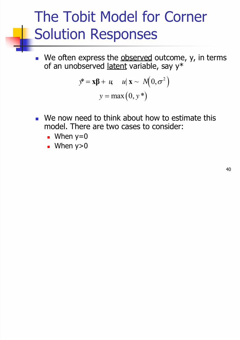
Solution Responses We often express the observed outcome, y, in terms
of an unobserved latent variable, say y*
We now need to think about how to estimate this
model. There are two cases to consider: When y=0
When y>0
( )
( )
2* , | ~ 0,
max 0, *
y u u N
y y
σ = +
=
xβ x
8/3/2019 09-Limited Dependent Variable Models
http://slidepdf.com/reader/full/09-limited-dependent-variable-models 41/71

8/3/2019 09-Limited Dependent Variable Models
http://slidepdf.com/reader/full/09-limited-dependent-variable-models 42/71
42
The Tobit Model for Corner
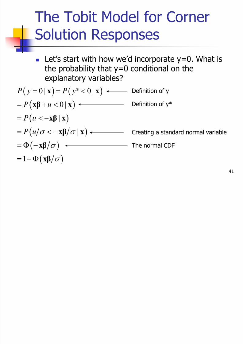
Solution Responses What is the probability that y>0 conditional on the
explanatory variables?
Since y is continuous for values greater than 0, theprobability is simply the density of the normalvariable u
We can now put together these two pieces to formthe log-likelihood function for the Tobit model (seeequation 17.22 in Wooldridge)
8/3/2019 09-Limited Dependent Variable Models
http://slidepdf.com/reader/full/09-limited-dependent-variable-models 43/71

8/3/2019 09-Limited Dependent Variable Models
http://slidepdf.com/reader/full/09-limited-dependent-variable-models 44/71
44
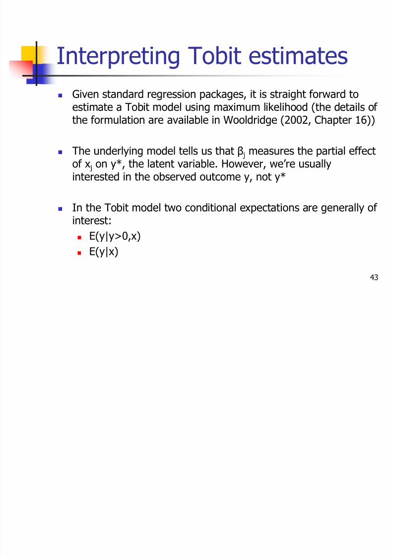
Interpreting Tobit estimates
Take home message: Conditional expectations in theTobit are much more complicated than in the linearmodel
E(y|x) is a nonlinear of function of both x and β.Moreover, this conditional expectation can be shownto be positive for any values of x and β.
( ) ( )
( ) ( ) ( )
| 0, /
| / /
E y y
E y
σλ σ
σ σφ σ
> = +
= Φ +
x xβ xβ
x xβ xβ xβ
8/3/2019 09-Limited Dependent Variable Models
http://slidepdf.com/reader/full/09-limited-dependent-variable-models 45/71
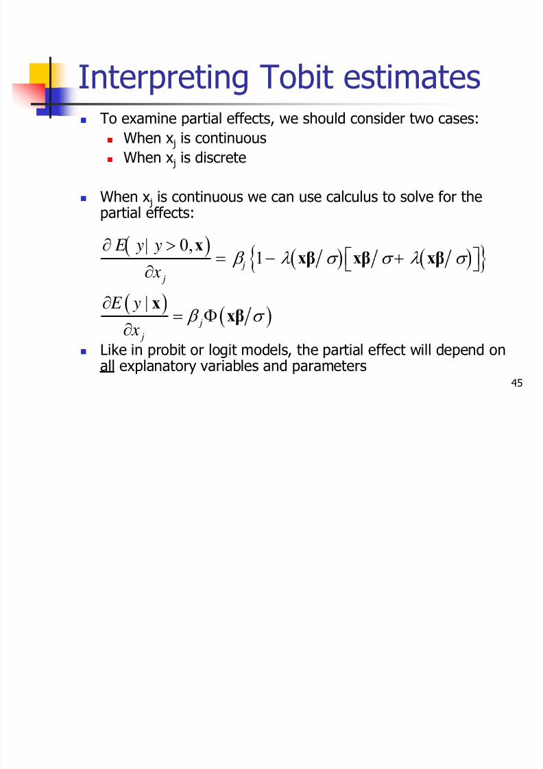
45
Interpreting Tobit estimates To examine partial effects, we should consider two cases:
When x j is continuous When x j is discrete
When x j is continuous we can use calculus to solve for the
partial effects:
Like in probit or logit models, the partial effect will depend onall explanatory variables and parameters
( )( ) ( ){ }
( )( )
| 0,1
|
j
j
j
j
E y y
x
E y
x
β λ σ σ λ σ
β σ
∂ >⎡ ⎤= − +⎣ ⎦∂
∂= Φ
∂
x
xβ xβ xβ
x
xβ

8/3/2019 09-Limited Dependent Variable Models
http://slidepdf.com/reader/full/09-limited-dependent-variable-models 46/71
46
Interpreting Tobit estimates When x
j
is discrete we estimate the partial effect asthe difference:
( ) ( )
( ) ( )
| 0, , 1 | 0, ,
| , 1 | ,
j j j j
j j j j
E y y x c E y y x c
E y x c E y x c
− −
− −
> = + − > =
= + − =
x x
x x

8/3/2019 09-Limited Dependent Variable Models
http://slidepdf.com/reader/full/09-limited-dependent-variable-models 47/71
47
Interpreting Tobit estimates Just like the probit and logit models, there are two
common approaches for evaluating the partialeffects:
Partial Effect at the Average (PEA)
Evaluate the expressions at the same average
Average Partial Effect (APE)
Calculate the mean over the values for the entire sample

8/3/2019 09-Limited Dependent Variable Models
http://slidepdf.com/reader/full/09-limited-dependent-variable-models 48/71
48
Example 17.2: Women’s
annual labour supply We can use the same dataset, MROZ.RAW, that we
used to estimate the probability of womenparticipating in the labour force to estimate theimpact of various explanatory variables on the total
number of hours worked
Of the 753 women in the sample:
428 worked for a wage during the year
325 worked zero hours in the labour market

8/3/2019 09-Limited Dependent Variable Models
http://slidepdf.com/reader/full/09-limited-dependent-variable-models 49/71
49
Tobit example: Women’s
annual labour supply reg hours nwifeinc educ exper expersq age kidslt6
kidsge6
tobit hours nwifeinc educ exper expersq age kidslt6kidsge6, ll(0)
8/3/2019 09-Limited Dependent Variable Models
http://slidepdf.com/reader/full/09-limited-dependent-variable-models 50/71
50
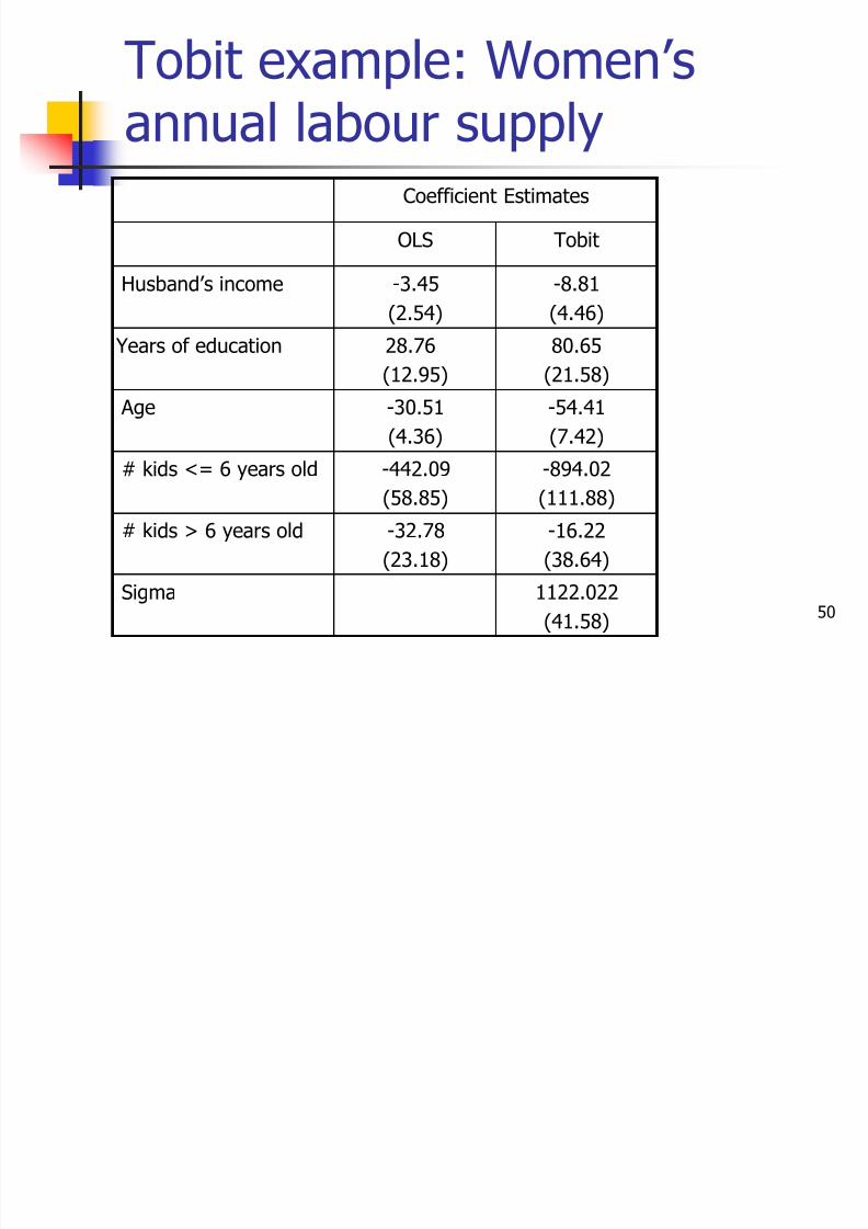
Tobit example: Women’s
annual labour supplyCoefficient Estimates
OLS Tobit
Husband’s income -3.45
(2.54)
-8.81
(4.46)
Years of education 28.76(12.95)
80.65(21.58)
Age -30.51
(4.36)
-54.41
(7.42)
# kids <= 6 years old -442.09
(58.85)
-894.02
(111.88)
# kids > 6 years old -32.78
(23.18)
-16.22
(38.64)Sigma 1122.022
(41.58)

8/3/2019 09-Limited Dependent Variable Models
http://slidepdf.com/reader/full/09-limited-dependent-variable-models 51/71
51
Tobit example: Women’s
annual labour supply The Tobit coefficient estimates all have the same sign
as the OLS coefficients
The pattern of statistical significance is also verysimilar
Remember though, we cannot directly compare theOLS and Tobit coefficients in terms of their effect onhours worked
b l ’
8/3/2019 09-Limited Dependent Variable Models
http://slidepdf.com/reader/full/09-limited-dependent-variable-models 52/71
52
Tobit example: Women’s
annual labour supply Let’s construct some marginal effects for some of the
discrete variables
First, the means of the explanatory variables:
Husband’s income: 20.12896
Education: 12.28685
Experience: 10.63081
Age: 42.53785
# young children: 0.2377158
# older children: 1.353254
b l ’
8/3/2019 09-Limited Dependent Variable Models
http://slidepdf.com/reader/full/09-limited-dependent-variable-models 53/71
53
Tobit example: Women’s
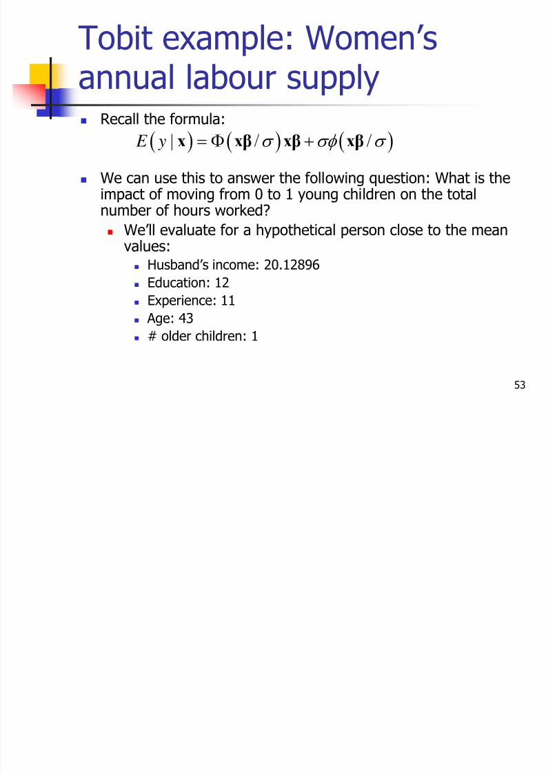
annual labour supply Recall the formula:
We can use this to answer the following question: What is theimpact of moving from 0 to 1 young children on the total
number of hours worked? We’ll evaluate for a hypothetical person close to the mean
values: Husband’s income: 20.12896
Education: 12 Experience: 11
Age: 43
# older children: 1
( ) ( ) ( )| / / E y σ σφ σ = Φ +x xβ xβ xβ
T bi l W ’
8/3/2019 09-Limited Dependent Variable Models
http://slidepdf.com/reader/full/09-limited-dependent-variable-models 54/71
54
Tobit example: Women’s
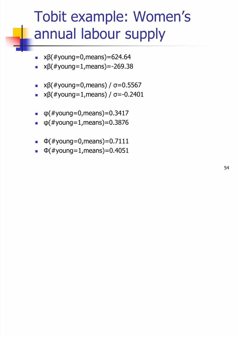
annual labour supply xβ(#young=0,means)=624.64
xβ(#young=1,means)=-269.38
xβ(#young=0,means) / σ=0.5567
xβ(#young=1,means) / σ=-0.2401
φ(#young=0,means)=0.3417
φ(#young=1,means)=0.3876
Φ(#young=0,means)=0.7111
Φ(#young=1,means)=0.4051
T bi l W ’

8/3/2019 09-Limited Dependent Variable Models
http://slidepdf.com/reader/full/09-limited-dependent-variable-models 55/71
55
Tobit example: Women’s
annual labour supply E(y|#young=0,means)=827.6
E(y|#young=1,means)=325.8
E(y|#young=0,means)-E(y|#young=1,means)=502
Thus, for a hypothetical “average” woman, going from 0 youngchildren to 1 young child would decrease hours worked by 502hours. This is larger than the OLS estimate of a 442 hourdecrease.
We could do the same thing to look at the impact of adding asecond young child.

8/3/2019 09-Limited Dependent Variable Models
http://slidepdf.com/reader/full/09-limited-dependent-variable-models 56/71
56
Specification Issues The Tobit model relies on the assumptions of normality and
homoskedasticity in the latent variable model
Recall, using OLS we did not need to assume a distributionalform for the error term in order to have unbiased (or consistent)estimates of the parameters.
Thus, although using Tobit may provide us with a more realisticdescription of the data (for example, no negative predictedvalues) we have to make stronger assumptions than when using
OLS.
In a Tobit model, if any of the assumptions fail, it is hard toknow what the estimated coefficients mean.
8/3/2019 09-Limited Dependent Variable Models
http://slidepdf.com/reader/full/09-limited-dependent-variable-models 57/71
57
Specification Issues One important limitation of Tobit models is that the expectation of y,
conditional on a positive value, is closely linked to the probability thaty>0
The effect of x j on P(y>0| x) is proportional to β j, as is the effect onE(y|y>0, x). Moreover, for both expressions the factor multiplying β j is
positive.
Thus, if you want a model where an explanatory variable has oppositeeffects on P(y>0| x) and E(y|y>0, x), then Tobit is inappropriate.
One way to informally evaluate a Tobit model is to estimate a probitmodel where: w=1 if y>0 w=0 if y=0
8/3/2019 09-Limited Dependent Variable Models
http://slidepdf.com/reader/full/09-limited-dependent-variable-models 58/71
58
Specification Issues The coefficient on x j in the above probit model, say
γ j, is directly related to the coefficient on x j in theTobit model, β j:
Thus, we can look to see if the estimated valuesdiffer.
For example, if the estimates differ in sign, this maysuggest that the Tobit model is in appropriate
j jγ β σ =
S ifi ti I A l
8/3/2019 09-Limited Dependent Variable Models
http://slidepdf.com/reader/full/09-limited-dependent-variable-models 59/71
59
Specification Issues: Annual
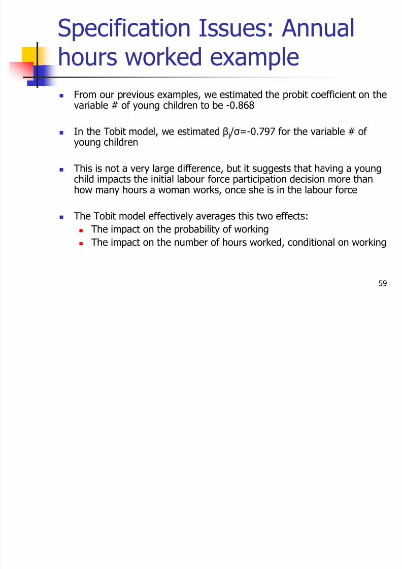
hours worked example From our previous examples, we estimated the probit coefficient on the
variable # of young children to be -0.868
In the Tobit model, we estimated β j /σ=-0.797 for the variable # of young children
This is not a very large difference, but it suggests that having a youngchild impacts the initial labour force participation decision more thanhow many hours a woman works, once she is in the labour force
The Tobit model effectively averages this two effects:
The impact on the probability of working
The impact on the number of hours worked, conditional on working

8/3/2019 09-Limited Dependent Variable Models
http://slidepdf.com/reader/full/09-limited-dependent-variable-models 60/71
60
Specification Issues If we find evidence that the Tobit model is
inappropriate, we can use hurdle or two-part models
These models have the feature that P(y>0|x) andE(y|y>0,x) depend on different parameters and thusx j can have dissimilar effects on the two functions(see Wooldridge (2002, Chapter 16))

8/3/2019 09-Limited Dependent Variable Models
http://slidepdf.com/reader/full/09-limited-dependent-variable-models 61/71
61
Practice questions 17.2, 17.3
C17.1, C17.2, C17.3
8/3/2019 09-Limited Dependent Variable Models
http://slidepdf.com/reader/full/09-limited-dependent-variable-models 62/71
62
Computer Exercise C17.2 Use the data in LOANAPP.RAW for this exercise.
Estimate a probit model of approve on white. Findthe estimated probability of loan approval for bothwhites and nonwhites. How do these compare to thelinear probability model estimates?
probit approve white
regress approve white

8/3/2019 09-Limited Dependent Variable Models
http://slidepdf.com/reader/full/09-limited-dependent-variable-models 63/71
63
Computer Exercise C17.2Probit LPM
White 0.784
(0.087)
0.201
(0.020)
Constant 0.547
(0.075)
0.708
(0.018)
• As there is only one explanatory variable and it takes only twovalues, there are only two different predicted probabilities: theestimated loan approval probabilities for white and nonwhite
applicants
•Hence, the predicted probabilities, whether we use a probit, logit, orLPM model are simply the cell frequencies:
•0.708 for nonwhite applicants•0.908 for white applicants

8/3/2019 09-Limited Dependent Variable Models
http://slidepdf.com/reader/full/09-limited-dependent-variable-models 64/71
64
Computer Exercise C17.2 We can do this in Stata using the following
commands following the probit estimation:
predict phat
summarize phat if white==1
summarize phat if white==0

8/3/2019 09-Limited Dependent Variable Models
http://slidepdf.com/reader/full/09-limited-dependent-variable-models 65/71
65
Computer Exercise C17.2 Now add the variables hrat, obrat, loanprc, unem,
male, married, dep, sch, cosign, chist, pubrec,mortlat1, mortlat2, and vr to the probit model. Isthere statistically significant evidence of
discrimination against nonwhites?

8/3/2019 09-Limited Dependent Variable Models
http://slidepdf.com/reader/full/09-limited-dependent-variable-models 66/71
66
Computer Exercise C17.2
approve
Coef.
Std. Err.
z
P>z
[95% Conf.Interval]
white
.5202525
.0969588
5.37
0.000
.3302168
.7102883
hrat
.0078763
.0069616
1.13
0.258
-.0057682
.0215209
obrat
-.0276924
.0060493
-4.58
0.000
-.0395488
-.015836
loanprc
-1.011969
.2372396
-4.27
0.000
-1.47695
-.5469881
unem -.0366849 .0174807 -2.10 0.036 -.0709464 -.0024234male
-.0370014
.1099273
-0.34
0.736
-.2524549
.1784521
married
.2657469
.0942523
2.82
0.005
.0810159
.4504779
dep
-.0495756
.0390573
-1.27
0.204
-.1261266
.0269753
sch
.0146496
.0958421
0.15
0.879
-.1731974
.2024967
cosign
.0860713
.2457509
0.35
0.726
-.3955917
.5677343
chist
.5852812
.0959715
6.10
0.000
.3971805
.7733818
pubrec
-.7787405
.12632
-6.16
0.000
-1.026323
-.5311578
mortlat1
-.1876237
.2531127
-0.74
0.459
-.6837153
.308468
mortlat2
-.4943562
.3265563
-1.51
0.130
-1.134395
.1456823
vr
-.2010621
.0814934
-2.47
0.014
-.3607862
-.041338
_cons
2.062327
.3131763
6.59
0.000
1.448512
2.676141

8/3/2019 09-Limited Dependent Variable Models
http://slidepdf.com/reader/full/09-limited-dependent-variable-models 67/71
67
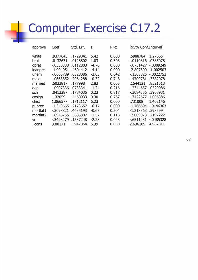
Computer Exercise C17.2 Estimate the previous model by logit. Compare the
coefficient on white to the probit estimate.
8/3/2019 09-Limited Dependent Variable Models
http://slidepdf.com/reader/full/09-limited-dependent-variable-models 68/71
68
Computer Exercise C17.2approve
Coef.
Std. Err.
z
P>z
[95% Conf.Interval]
white
.9377643
.1729041
5.42
0.000
.5988784
1.27665
hrat
.0132631
.0128802
1.03
0.303
-.0119816
.0385078
obrat
-.0530338
.0112803
-4.70
0.000
-.0751427
-.0309249
loanprc
-1.904951
.4604412
-4.14
0.000
-2.807399
-1.002503
unem
-.0665789
.0328086
-2.03
0.042
-.1308825
-.0022753
male
-.0663852
.2064288
-0.32
0.748
-.4709781
.3382078
married
.5032817
.177998
2.83
0.005
.1544121
.8521513
dep
-.0907336
.0733341
-1.24
0.216
-.2344657
.0529986
sch
.0412287
.1784035
0.23
0.817
-.3084356
.3908931
cosign
.132059
.4460933
0.30
0.767
-.7422677
1.006386
chist
1.066577
.1712117
6.23
0.000
.731008
1.402146
pubrec
-1.340665
.2173657
-6.17
0.000
-1.766694
-.9146363
mortlat1
-.3098821
.4635193
-0.67
0.504
-1.218363
.598599
mortlat2
-.8946755
.5685807
-1.57
0.116
-2.009073
.2197222
vr
-.3498279
.1537248
-2.28
0.023
-.6511231
-.0485328
_cons
3.80171
.5947054
6.39
0.000
2.636109
4.967311

8/3/2019 09-Limited Dependent Variable Models
http://slidepdf.com/reader/full/09-limited-dependent-variable-models 69/71
69
Computer Exercise C17.2 Use the average partial effect (APE) to calculate the
size of discrimination for the probit and logitestimates.

8/3/2019 09-Limited Dependent Variable Models
http://slidepdf.com/reader/full/09-limited-dependent-variable-models 70/71
70
Computer Exercise C17.2 This can be done in Stata using the user-written
command margeff For dummy variables the APE is calculated as a
discrete change in the dependent variable as thedummy variable changes from 0 to 1 (see Cameronand Trivedi, 2009, Chapter 14)
probit
...
margeff
logit ...
margeff

8/3/2019 09-Limited Dependent Variable Models
http://slidepdf.com/reader/full/09-limited-dependent-variable-models 71/71
Computer Exercise C17.2 Average Partial Effect of being White on Loan
Approval
Probit Logit OLS
White 0.104(0.023)
0.101(0.022)
0.129(0.020)
Partial Effect at the Average
White 0.106
(0.024)
0.097
(0.022)
0.129
(0.020)

![LIMITED DEPENDENT VARIABLES - BASICminiahn/ecn726/cn_limited.pdf · 2006. 10. 27. · LIMITED DEPENDENT VARIABLES - BASIC [1] Binary choice models • Motivation: • Dependent variable](https://static.fdocuments.us/doc/165x107/60f7d4918b31c671c84c8122/limited-dependent-variables-miniahnecn726cnlimitedpdf-2006-10-27-limited.jpg)