09-02 FRONT COVER - steinhardt.nyu.edu Working... · WORKING PAPER #09-05 April 2009....

IESP Working Paper Series

Risk Aversion and Support for Merit Pay: Theory and Evidence from Minnesota's Q Comp Program

Carl NadlerResearch DepartmentFederal Reserve Bank of Boston

Matthew WiswallDepartment of EconomicsNew York University

WORKING PAPER #09-05April 2009

Acknowledgements

.

Editorial Board

The editorial board of the IESP working paper series is comprised of senior research staff and affiliated faculty members from NYU's Steinhardt School of Culture, Education, and Human Development and Robert F. Wagner School of Public Service. The following individuals currently serve on our Editorial Board:

Amy Ellen Schwartz Director, IESP

NYU Steinhardt and NYU Wagner

Sean Corcoran NYU Steinhardt

Cynthia Miller-Idriss

NYU Steinhardt

Leslie Santee Siskin NYU Steinhardt

Leanna Stiefel

Associate Director for Education Finance, IESP NYU Wagner

Mitchell L. Stevens

NYU Steinhardt

Sharon L. Weinberg NYU Steinhardt

Beth Weitzman

NYU Wagner

The views expressed in this paper are those of the authors and do not necessarilyrepresent those of the Federal Reserve Bank of Boston or the Federal Reserve System. We thank Tavis Barr, Mary Burke, Rajashri Chakrabarti, Julie Berry Cullen, Jane Katz, Randy Reback, Jennifer Sallman, Leanna Stiefel, and Patrick Walsh for helpful comments.

Abstract

Recent research attributes the lack of merit pay in teaching to the resistance of teach-ers. This paper examines whether the structure of merit pay affects the types of teach-ers who support it. We develop a model of the relative utility teachers receive from merit pay versus the current fixed schedule of raises. We show that if teachers are riskaverse, teachers with higher base salaries would be more likely to support a merit pay program that allows them to keep their current base salary and risk only future salary increases. We test the predictions of the model using data from a new merit pay program, the Minnesota “Q Comp" program, which requires the approval of the teach-ers in each school district. Consistent with the model's predictions, we find that districts with higher base salaries and a higher proportion of teachers with masters degrees are more likely to approve merit pay.

1 Introduction

One of the more prominent findings in the recent education literature is the

wide distribution of teacher quality. Using administrative datasets that in-

clude classroom teachers and their students’ test scores, a number of studies

have documented large differences in the measured effectiveness of teachers,

even when accounting for the non-random sorting of teachers across schools

and other confounding education inputs.2 This variation in teacher quality

has prompted calls to reform how teachers are licensed, hired, and compen-

sated. One such reform, often referred to as “merit pay” or “performance

pay,” links teacher compensation to measures of performance. In most public

schools, teacher compensation is based almost entirely on years of experience

and accumulated graduate education credits and degrees earned (Lankford

and Wycoff 1997; Allegretto, Corcoran, and Mishel 2004). The goal of merit

pay is to create incentives for teachers to increase their level of teaching effort

and encourage better teachers to enter and stay in teaching (Podgursky and

Springer 2007). Despite the expectation that basing teacher compensation

at least in part on merit considerations may improve education outcomes,

merit pay programs have been estimated to exist in only about 10 percent of

public schools, and the existing programs are often limited in the proportion

2See Hanushek and Rivkin (2006), Wayne and Youngs (2003), and Hanushek (1997) forsummaries of the recent literature. Examples of the most recent research include: Clotfel-ter, Ladd, and Vigdor (2006) using data for North Carolina; Hanushek, Kain, and Rivkin(2005) using data for Texas; Rockoff (2004) using data for New Jersey; and Aaronson,Barrow, and Sander (2003) using data for Chicago; Nye, Konstantopoulos, and Hedges(2004) using data for Tennessee; and Boyd et al (2006) using data for New York City.

1

IESP Working Paper #09-05

of compensation that is tied to performance (Ballou and Podgursky 1993;

Ballou 2001).3

Earlier research on the reasons for the lack of merit pay in the teaching

profession has reached mixed conclusions. Murnane and Cohen (1986) pre-

sented some of the earliest findings using case studies of 6 school districts

that had merit pay programs and concluded that the teaching profession

is not suitable for merit pay. Referencing the literature on personnel eco-

nomics, they argued that there are multiple goals of teaching, some of which

cannot be measured, and basing teacher pay on the measurable goals creates

incentives to neglect the others. In addition, to the extent that there is a

team component to teaching, merit pay creates disincentives for cooperation

among teachers. Murnane and Cohen (1986) concluded that merit based

compensation works only under very special circumstances: small school dis-

tricts, with homogeneous populations and high base salaries, and where the

performance bonuses are small. Later research by Ballou and Podgursky

(1993) disputed this conclusion. Ballou and Podgursky argued that the lack

of merit pay in public schools is due to the opposition of teachers and their

unions, rather than a fundamental unsuitability of teaching for merit pay.

Ballou and Podgursky (1993) cited a number of attempts to create merit pay

plans in the 1980s that were ultimately derailed by opposition from teacher’s

unions. As further evidence of this, Ballou (2001) examined the 1993-94

3Some compensation in teaching may be indirectly tied to performance as in thecase where administrators provide additional pay for selected teachers to supervise extra-curricular activities or serve as department chairs or mentors for other teachers.

2


School and Staffing Surveys (SASS) and found that 20 percent of school dis-

tricts where unions are not present have merit pay programs, compared to 8

percent of school districts where unions have the right of collective bargain-

ing. Goldhaber et al (2008) using SASS 2000 data also find that unionization

reduces the incidence of merit pay.4

In recent years, teachers’ unions have begun working with policymakers

to develop merit pay programs. Reflecting this change, Randi Weingarten,

the current president of the American Federation of Teachers, has stated that

her union is open to education reforms including merit pay.5 The products

of this collaboration, including Denver’s ProComp, Minnesota’s Q Comp,

and Florida’s Merit Awards Program, differ from earlier merit pay programs

in that teachers can, either individually or collectively through their school

district, choose whether to change their compensation.

In this paper, we use the recent experience of the Q Comp (“Quality

Compensation for Teachers”) program in Minnesota to examine the condi-

tions under which teachers would voluntarily accept a merit pay basis for

compensation. A distinguishing feature of this program is that before a Q

Comp plan can be implemented in a district, the program needs the ap-

4To test whether more information on teaching performance might independently leadto the adoption of merit pay, Goldhaber et al (2008) also examine the relationship betweendistrict use of accountability standards and the incidence of merit pay. While accountabil-ity standards might plausibly change the nature of teaching by providing districts withmore information about teacher performance, they find no relationship between account-ability standards and merit pay adoption.

5Dillon, Sam; “Head of Teachers’ Union Offers to Talk on Tenure and Merit Pay,” NewYork Times, November 17, 2008.

3


proval of a district’s teachers, usually by a majority vote of the teachers.

Understanding the nature of teacher opposition to merit pay may help us

design merit pay programs that both improve educational outcomes and are

acceptable to enough teachers to win approval.

The analysis in this paper contributes to the literature in two ways. First,

incorporating the uncertainty that teachers face in a switch to merit pay, we

develop a theoretical model of the utility risk averse teachers receive from

merit pay relative to the current fixed schedule. Second, rather than use

surveys of teacher attitudes toward hypothetical merit pay programs, we use

actual district level approvals of the Q Comp program to explicitly provide

information on the conditions under which teachers would voluntarily accept

a merit pay reform.6

A distinguishing feature of our analysis is that we focus on heterogeneity

in the types of teachers who would gain from a switch to merit pay. Our

analysis complements the recent theoretical and empirical analysis of Gold-

haber et al (2008), which examines the district’s decision to offer merit pay.

In their model, the district offers merit pay if the gains in student achieve-

ment outweigh the political costs and the higher wages that the district may

have to offer teachers to compensate them for the uncertainty in compensa-

tion merit pay introduces. Their model is more general in the sense that a

teacher’s effort decision and the gains to merit pay to districts are explicitly

6We do not discuss the optimal merit pay program or the effects of merit pay on theteacher labor market. For an overview of these issues, see Podgursky and Springer (2007).

4


considered. However, in Goldhaber et al (2008) teachers are homogeneous

with respect to base pay and other characteristics as merit pay simply affects

the level and certainty of wages uniformly for all teachers. In addition, they

do not consider differences in the structure of merit pay and how these differ-

ences might appeal to different kinds of teachers, depending on the teacher’s

current base pay due to different levels of experience and education.

In our model, we find an important difference between a merit pay pro-

gram that bases all future salary on performance, and a program, like Q

Comp, that guarantees teachers that their future salary will not fall below

their current salary. We find that if teachers are risk averse and future com-

pensation is sufficiently risky, teachers with higher base salaries under the

current schedule will have larger gains from a switch to a merit pay pro-

gram that allows teachers to retain their current base salaries since a smaller

proportion of future salary is at risk. This implies that more experienced

teachers and teachers with higher levels of graduate education, who have

higher salaries under the current system, would be more likely to favor a Q

Comp type merit pay program than younger teachers and teachers with only

bachelors degrees. Underscoring this feature of Q Comp, when we examine

a general merit pay program that bases all future salary on performance,

we find the opposite pattern, as teachers with higher salaries before merit

pay implementation have more to lose from the switch. This theoretical

prediction is consistent with research by Ballou and Podgursky (1993) who

examined a survey of teachers’ attitudes toward a hypothetical general merit

5


pay program (the 1987-88 School and Staffing Surveys). They found that

teachers with masters degrees and more experience were more likely to op-

pose merit pay.

We test the predictions of the model by using district level information

on the characteristics of teachers and students for Minnesota school districts.

A significant finding from the empirical analysis is that Q Comp approval is

more likely in school districts with higher salaries and a higher percentage

of teachers who hold masters degrees. Although we cannot rule out the

possibility of omitted variable bias from the unobservable characteristics,

when we conduct a multivariate analysis including characteristics of each

district’s students, their surrounding communities, and other characteristics

of the district’s teachers, these findings prove to be robust.

The Q Comp program reverses the traditional opposition to merit pay

programs from those teachers who gain under the fixed salary schedule. Un-

der a program like Q Comp, most of the risk is borne by low base salary

teachers as a greater proportion of their future compensation will be based

on performance. By mandating that no teacher’s salary will be lowered as

a result of their district approving Q Comp, many of the disincentives from

leaving the fixed salary schedule for teachers who benefit from this schedule

are removed. The Q Comp merit pay program in effect re-calculates the

political economy of merit pay by shifting the risk of merit pay onto inexpe-

rienced teachers and teachers with only bachelors degrees. This may explain

the relative political viability of the Q Comp merit pay program and indicate

6


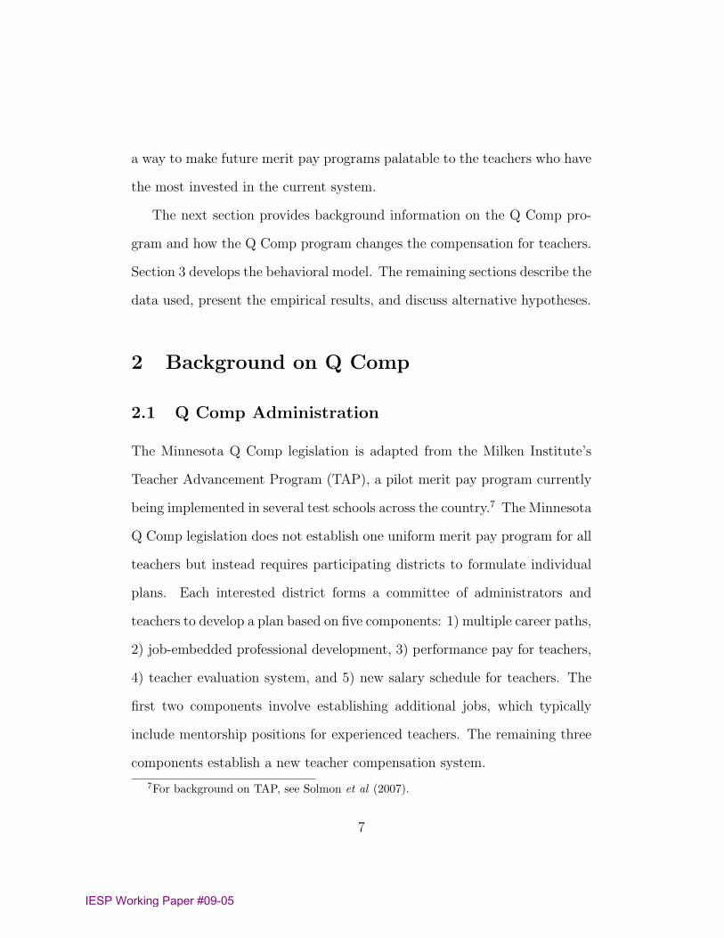
a way to make future merit pay programs palatable to the teachers who have

the most invested in the current system.

The next section provides background information on the Q Comp pro-

gram and how the Q Comp program changes the compensation for teachers.

Section 3 develops the behavioral model. The remaining sections describe the

data used, present the empirical results, and discuss alternative hypotheses.

2 Background on Q Comp

2.1 Q Comp Administration

The Minnesota Q Comp legislation is adapted from the Milken Institute’s

Teacher Advancement Program (TAP), a pilot merit pay program currently

being implemented in several test schools across the country.7 The Minnesota

Q Comp legislation does not establish one uniform merit pay program for all

teachers but instead requires participating districts to formulate individual

plans. Each interested district forms a committee of administrators and

teachers to develop a plan based on five components: 1) multiple career paths,

2) job-embedded professional development, 3) performance pay for teachers,

4) teacher evaluation system, and 5) new salary schedule for teachers. The

first two components involve establishing additional jobs, which typically

include mentorship positions for experienced teachers. The remaining three

components establish a new teacher compensation system.

7For background on TAP, see Solmon et al (2007).

7


The Q Comp law requires that the proposed salary schedule have at

least 60 percent of all future salary increases aligned with evaluated teacher

performance. Current salary levels for incumbent teachers are unaffected,

and future salaries cannot fall below the current base salary. In the third

component, districts are required to establish a teacher evaluation system,

which the law states can be based on a combination of peer or supervisor

evaluations and student gains on state examinations.

Once a district completes its proposed plan, the Q Comp law requires the

district to obtain the approval of the head of the local teachers’ union and

the superintendent or school board chair before the plan is sent to the state

for approval. The state has thirty days to evaluate the plan to make sure it

contains the five components described above. If the submitted plan does not

meet these requirements, the district is given thirty days to revise the plan. If

the revised plan still does not meet the requirements of the Q Comp program,

the district’s plan is rejected. According to the Minnesota Department of

Education, most districts are asked to revise their plans, however, only five

have been rejected.8 Upon acceptance by the state, the districts’ teachers

vote on the plan according to their district’s collective bargaining agreement.

Only four districts’ teachers have voted down an approved Q Comp proposal.9

8Several plans from charter schools have also been rejected. Because charter schoolsoften operate very differently from non-charter schools, we exclude charter school districtsin our empirical analysis.

9Because of Q Comp’s novelty and controversy, the above process is heavily dissectedin local and major newspapers in Minnesota. The public in general knows whether theirdistrict is proposing a plan, and we expect that districts that send plans for state approvalalready believe that their plan will be approved by their district’s teachers in the final

8


In the 2005-06 school year, the first year Q Comp was employed, nine school

districts participated. By March 2007, 34 districts had joined for the 2006-07

school year. Appendix A provides a complete list of participating districts.

2.2 Salary Schedules

The traditional teacher salary schedule awards teachers a higher wage for

more years of experience and education. Figure 1 plots the average wage

schedule for the Q Comp school districts before they approved their Q Comp

plan (2006-07). As the size and number of salary increments based on expe-

rience vary among districts, we compute the mean step increases separately

for years 0 - 10, 10 - 20, and 20 and more.10 In Figure 1 we plot the average

salary schedules for teachers with bachelors and masters degrees. Teachers

with only a bachelors degree earned an average starting salary of $31,595,

and had salary step increases of $920 for the first 10 years, $451 during the

next 10 years, and $225 thereafter. Teachers with masters degrees had a

higher starting salary of $35,983, and had $1,329 step increases during the

first 10 years, $743 during the next ten years, and $345 thereafter.11

We next examine the specific details of the Q Comp plans using data

obtained from approval letters for participating districts. The letters describe

approval process.10The number of steps in the Q Comp districts prior to Q Comp reform range from 12

to 43, with mean 24.54 and standard deviation 6.98.11Teachers often can earn higher wages for completing graduate coursework leading up

to, and beyond, a masters degree.

9


how participating in Q Comp affects teachers’ salaries.12 The level of detail

described in these approval letters vary, and we were not able to record data

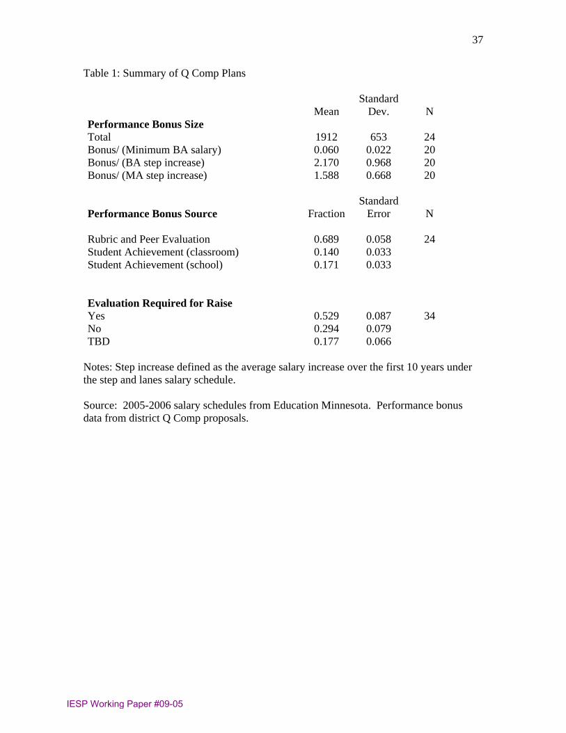
for all districts. As indicated in Table 1, participating districts on average

offered teachers $1,912 in one-time performance bonuses that are not carried

over the next year. Almost 70 percent of this amount is earned through

receiving a positive performance review from the teacher’s supervisors. The

remaining portion is divided between the teacher’s students’ achievement and

school-wide student achievement.

One concern for merit pay reform in public schools is the size of the

performance incentives. Ballou (2001) finds using the 1990-91 SASS that

public schools on average awarded their teachers a mere 2 percent of base

salary, compared to about 10 percent in non-sectarian private schools. As

summarized in Table 1, the $1,912 average Q Comp bonus is 6 percent of the

average starting salary for a teacher with a bachelors degree.

Although the Q Comp law only requires school districts to offer one-time

performance bonuses and allows districts to maintain their fixed salary sched-

ule, as detailed in Table 1 more than half of participating districts require

teachers to have a positive performance evaluation for earning future raises

on a salary schedule. A few of these districts, such as Eden Praire and Grand

Meadow, have dismantled the traditional salary schedule entirely, replacing

it with a combination of potential performance-based permanent salary aug-

12See the Data Appendix for details on how we used the letters to determine the datavalues summarized in this table.

10


mentations and one-time bonuses. Most of the districts maintain the salary

schedule and require a positive performance evaluation before receiving a

permanent salary augmentation, in addition to offering performance-based,

one-time bonuses.13

Regardless of which method used, the teachers in Q Comp districts have

voluntarily implemented a merit pay system that introduces an element of

uncertainty into teacher salaries. Table 1 illustrates that in every district Q

Comp reform introduces uncertainty into teachers’ future incomes, although

the amount of risk teachers incur varies among districts. With Q Comp, fund-

ing originally reserved for wages that were guaranteed is now divided between

fixed and performance-based augmentations. Bonuses are in part a function

of peer and administrator evaluations that are difficult to predict before Q

Comp implementation. Additionally, bonuses depend on uncertain student

performance. Finally, more than half of Q Comp districts require that future

permanent salary increases are conditional on a positive performance review.

Depending on the degree of teacher risk aversion, this uncertainty in future

salaries could have important implications for how teachers value Q Comp

relative to the certainty of the fixed wage schedule.

13 Mounds View’s and LaCrescent-Hokah’s Q Comp programs are examples of suchreform.

11


3 Model

This section develops a model of the utility teachers receive from a general

merit pay program relative to the current fixed schedule of pay raises. We

use this model to examine which types of teachers would favor merit pay

over the current compensation schedule and how the structure of the merit

pay program affects this support. The empirical sections below test these

predictions using data on the school districts that have and have not approved

a Q Comp merit pay program.

3.1 Wage Schedules

We first specify the wage schedules under the two systems for a given teacher.

Teachers are assumed to be heterogeneous in their current base pay. To focus

on the issue of how a merit pay program is valued by currently employed

teachers, we assume individuals work as teachers for their entire career until

an exogenous retirement date. We leave for future research the issue of how

merit pay reforms affect the recruitment and career length of teachers.

When the merit pay plan is offered, the teacher is in year τ of her career

with τ years of teaching experience. The teacher’s base salary as they enter

period τ is given by w0. In each year, salaries under the fixed schedule, from

the current period t = τ until the exogenous retirement date in period t = T ,

are given by

12


wFt = w0 + vt. (1)

vt ≥ 0 for all t is the cumulative step increase in the salary schedule for

each period that is added onto each teacher’s base salary at period t. The vt

step increase reflects any increase in salary from the initial level of base pay

w0.14

The alternative merit pay program replaces the fixed schedule of salary

increases with stochastic performance bonuses. The total salary teachers

receive in each year of the merit pay program consists of some fraction γ ∈

[0, 1] of their base salary plus a temporary performance bonus bt ≥ 0. The

salary for teachers under merit pay for t = τ, . . . , T is given by

wMt = γw0 + bt. (2)

γ indicates the proportion of their base salary that teachers are allowed

to keep after the start of the merit pay program. If all salary is based on

performance bonuses, γ = 0. With γ = 0, the merit pay program essentially

re-sets all teacher salaries to the same level and eliminates any gains in salary

teachers may have accumulated through obtaining graduate education or

14For simplicity, we assume that the salary step increases vt do not vary with base salaryw0, as with wFt = w0 + vt(w0). From the discussion of salary schedules above, we knowthat in Minnesota on average, teachers with bachelors and masters degrees (who havedifferent base salaries) have different salary step increases. In general, the model could beexpanded to allow for differences in salary step increases without changing the qualitativepredictions. In this more general case, a teacher’s relative utility over merit pay woulddepend not only on the level of their current base pay but also the year of their career τsince this determines the future salary increases the teacher expects on the fixed schedule.

13


years of education. All salaries under this type of merit pay depend solely on

performance bonuses. In the Minnesota Q Comp program, γ = 1, as future

salaries are not allowed to fall below the teacher’s base salary. Future salaries

under this type of merit pay then depend on the current level of base pay

and future performance bonuses.

3.2 Relative Utility from Merit Pay

We next define the utility teachers receive from merit pay relative to the

current fixed schedule. The utility function is assumed to be a Constant

Relative Risk Aversion function in current salaries: u(w) = w1−ρ

1−ρ , where

ρ ∈ [0,∞) measures the extent of risk aversion. As τ indicates the years of

teaching experience a teacher currently has when the merit pay program is

offered, a teacher has T − τ +1 remaining years in teaching. With a discount

rate of δ ∈ (0, 1), the sum of discounted utility under the fixed schedule is

UF (w0) =T∑t=τ

δt−τu(wFt). (3)

For the merit pay program, the discounted sum of expected utility is

UM(w0) =T∑t=τ

δt−τEb[u(wMt)], (4)

where Eb indicates expectations with respect to the stochastic perfor-

mance bonuses. We assume a simple distribution for the stochastic bonuses.

Bonus are distributed independently over time, with distribution bt = bH

14


(high bonus) with probability π ∈ (0, 1) and bt = bL (low bonus) with prob-

ability 1 − π. We assume the support of the bonus bounds the increase in

the fixed salary schedule: bH > vt > bL for all t. This assumption implies

that the merit pay bonus involves both a reward (bH) that is higher than

the current schedule of raises and a punishment (bL) that is lower than the

current schedule of raises.15

For a teacher with a base pay of w0, we measure the relative utility

from merit pay, or the “gains” from merit pay, using the difference in ex-

pected discounted lifetime utility between the two salary schedules for teach-

ers: ∆(w0) ≡ UM(w0) − UF (w0). A teacher with base pay w0 would favor

merit pay if ∆(w0) > 0.

3.3 Base Pay and Support for Merit Pay

We next consider how the relative utility from merit pay depends on the

teacher’s base pay under various merit pay structures (vary γ) and degrees

of teacher risk aversion (vary ρ). We first consider the case in which the

merit pay program does not allow teachers to keep their base pay (γ = 0).

Under this type of merit pay plan, we have the following result:

15The model could be generalized to allow for a floor on teacher salaries such thatteacher salaries never fall below teacher salary floor of w̄ < w0. With the imposition of asalary floor, salaries from merit pay are wMt = w̄ if γw0 + bt < w̄ and γw0 + bt otherwise.At γ = 0, the merit pay system still guarantees teachers a salary floor of w̄. With γ = 1,merit pay salaries are defined as above (2): wMt = w0 + bt. The simulation below setssuch a salary floor since it seems reasonable that even in a merit pay system with γ = 0,teachers would be guaranteed a minimum salary. However, as the simulation shows, sucha change to the model does not alter the qualitative results.

15


Proposition 1 If teachers are not allowed to keep their base pay, teachers

with higher base salaries would have lower relative utility from merit pay, for

any degree of risk aversion.

Proof Differentiating ∆(w0) with respect to base pay w0, we have

∂∆(w0)

∂w0

=T∑t=τ

δt−τ{πγ(γw0 + bH)−ρ + (1− π)γ(γw0 + bL)−ρ − (w0 + vt)−ρ}

Specializing to γ = 0 yields

∂∆(w0)

∂w0

= −T∑t=τ

δt−τ (w0 + vt)−ρ.

For any ρ ∈ [0,∞), ∂∆(w0)∂w0

< 0. QED

The intuition for this result is that teachers who have reached a high

base salary (e.g. because they are experienced or have a masters degree),

have more to lose from a merit pay program that disregards current base

salaries and sets future salaries based solely on stochastic bonuses. This

result provides some insight into why experienced teachers and teachers with

masters degree historically have greater opposition to merit pay programs

that would not allow them to keep their base salaries.

Next, we consider the case in which teacher are allowed to keep their

full base pay (γ = 1). Under this merit pay system, the gains to merit pay

depend on the degree of risk aversion. If teachers are risk neutral, we have

the following result:

16


Proposition 2 If teachers are allowed to keep their current base pay and

are risk neutral, then the gains to merit pay are flat with respect to base pay.

Proof With γ = 1,

∂∆(w0)

∂w0

=T∑t=τ

δt−τ{π(w0 + bH)−ρ + (1− π)(w0 + bL)−ρ − (w0 + vt)−ρ}.

With ρ = 0, we have

∂∆(w0)

∂w0

=T∑t=τ

δt−τ{π + (1− π)− 1} = 0.

QED

From Proposition 2 we conclude that base salary has no relationship to

support for merit for risk neutral teachers who can keep their base pay.

However, if teachers can keep their base pay and are risk averse (ρ > 0),

support for merit pay can be increasing or decreasing in base pay. How the

support for merit pay relates to base pay depends on the particular structure

of the merit pay program: the bonus size (bL, bH) and the probability of

obtaining the bonus (π). Given some bonus sizes bL, bH , we have the following

result:

Proposition 3 If teachers are risk averse and can keep their base pay, sup-

port for merit pay is increasing in base pay if the probability of obtaining the

17


bonus π is π < π∗, and decreasing in base pay otherwise, where

π∗ =T∑t=τ

δt−τ(w0 + bL)−ρ − (w0 + vt)

−ρ

(w0 + bL)−ρ − (w0 + bH)−ρ∈ (0, 1).

Proof See Appendix.

Proposition 3 states that if the probability of receiving the bonus is suf-

ficiently low relative to the size of the bonus, then, for risk averse teachers,

the gains to merit pay are increasing in their level of base pay. A key insight

is that this result is due to both a feature of the merit pay program (i.e.

being allowed to keep their base pay) and teachers’ preferences toward risk.

Comparing this result to Proposition 1 and 2, we see that if teachers are

either risk neutral or cannot keep their base pay, this result does not hold,

and the gains to merit pay are weakly decreasing in base pay.

3.4 Simulation

Figure 2 shows the results of a simulation of the model. In this simulation,

we examine teachers with 20 years of experience (τ = 20) and assume the

fixed schedule has salary increases of vt = $100 ∗ t. The merit pay program

has bonuses bL = 0 and bH = $2, 000 with probability of the high bonus set

at π = 0.1.16 We set the remaining parameters at δ = 0.95 and T = 35.

16In all of the simulations, we assume that a teacher’s salary cannot fall below $25,000.Salaries under merit pay are then wMt = 25, 000 if γw0 + bt < 25, 000 and γw0 + btotherwise. As discussed above, this places a realistic floor on salaries even if teachers arenot allowed to keep their full base salary (γ = 0).

18


We simulate the gains from merit pay (∆) using 5,000 draws from the bonus

distribution and varying the level of the base pay from $30,000 to $50,000.

Figure 2 demonstrates the range of possible teacher gains from merit

pay under four different combinations of parameters: i) ρ = 0, γ = 0, ii)

ρ = 3, γ = 0, iii) ρ = 0, γ = 1, and iv) ρ = 3, γ = 1. The vertical axis of

Figure 2 measures the gains in merit pay in terms of the proportional change

in ∆(w0) relative to the level at a base salary of $30,000: |∆(w0)−∆(w0 =

30, 000)|/|∆(w0 = 30, 000)|. Positive values of this metric indicate that the

gains to merit pay are higher for teachers with higher levels of base pay. This

relative gains metric allows us to abstract from the less controversial insight

that, all else being equal, a higher bonus level and more favorable odds of

obtaining the bonus attract greater teacher support.

Figure 2 indicates that if teachers cannot keep their base pay (γ = 0),

the gains to merit pay are declining in the level of base pay (Proposition 1).

However, an interesting element of the simulation is that the rate of decline

is smaller for risk averse teachers (ρ = 3) than for risk neutral teachers

(ρ = 0). This indicates that the more risk averse teachers are, the more

the favor the fixed schedule over a merit pay system where they cannot keep

their base salary. For teachers who are risk neutral and can keep their base

pay, the gains are flat with respect to base pay (Proposition 2). In this

simulation, the merit pay bonuses are sufficiently risky that the gains to

merit pay are increasing for risk averse teachers under a merit pay program

where teachers can keep their current base pay (Proposition 3). Only with

19


risk averse teachers and a particular structure to the merit pay program are

the gains increasing with respect to base pay.

4 Data

The theoretical model provides hypotheses about the relationship between

the gains from merit pay and characteristics of teachers. As described in

this section, we have access to district level data for the state of Minnesota

that includes whether the district approved a Q Comp merit program and

information about the characteristics of the specific merit pay program. We

match these data to district level data on the characteristics of the teachers,

students, and wage schedules at each district.

The data we use come from the Minnesota Department of Education

(MDE) and National Center of Education Statistics Common Core of Data

(CCD). The MDE provides information on which districts voted in favor of a

Q Comp program for the 2005-06 and 2006-07 school years. Although teacher

level voting data for Q Comp approval would be desirable, these data were

not collected by the state of Minnesota.17

The MDE provides annual information on the characteristics of teachers

17We also have no information on the exact approval criteria required by the teacher’sunions in each districts. As discussed above, the Q Comp law specifies that each schooldistrict’s teachers need to approve the Q Comp law according to their union rules. Wedo not know the specifics of this approval process, but conversations with administratorslead us to believe that approval requires at least a majority of teachers to vote in favorof the proposal. With a dataset of school districts, we estimate the probability a districtapproves Q Comp conditional on observed district characteristics. However, it is unlikelythese voting criteria vary systematically by any of the other explanatory variables.

20


within each district including the proportion of teachers within each dis-

trict that have a masters or PhD degree, and the age, gender, and racial

composition of teachers within the district. The salary data provided by the

MDE includes average salary for all teachers, starting salary for inexperienced

teachers with a bachelors degree, and the maximum salary for experienced

teachers with and without a masters degree. The MDE also provides data

on school district results on yearly state examinations called the Minnesota

Comprehensive Assessment (MCA). In 2003, the MDE reported scores on

the MCA for third and fifth grade students on the reading and mathematics

tests. As a measure of the proportion of high achieving students, we use the

proportion of 5th grade students who earned the highest level on the reading

MCA.18 The MDE also provides the student attendance rate for each district.

The CCD provides a number of additional district level variables includ-

ing student-to-teacher ratios, the proportion of students receiving free or

reduced price lunch, the racial composition of the students, and per student

expenditure. The CCD also includes data from the 2000 Population Census

on the demographic and income composition of the district’s surrounding

community.

Our sample of school districts excludes 54 charter, special education, and

other specialized school districts. In addition, we exclude 11 school districts

with missing district level characteristics. The remaining sample includes 328

Minnesota school districts, 34 of which had approved a Q Comp program by

18Similar results are found using the mathematics MCA.

21


March 2007. All school districts that we record as having approved a Q

Comp program did so between the beginning of the program in 2005-06 and

March 2007. Some school districts may approve Q Comp in the future either

because of changes in the composition of students or teachers in the districts

or because some school district teachers are undecided as to how Q Comp

would affect them and are waiting for more information. We take the 34

districts that have already approved Q Comp as an indication that they are

more in favor of Q Comp than the remaining districts. The matched district

level data from the MDE and CCD is for the 2004-05 school year, 2004 budget

year, 2003 test year, and 2000 Census. The district level characteristics are

constructed using the most recent data available preceding the approval of

Q Comp.19

5 Empirical Results

We use district-level data on Minnesota’s Q Comp program to test our

model’s predictions. As discussed in Section 2.2, the fixed salary schedule

rewards more educated and experienced teachers with higher base salaries.

Our model predicts that districts with higher overall salaries and districts

with more educated and experienced teachers who have higher base salaries

will be more likely to approve Q Comp.

1974 school districts are missing data on salary information for their teachers. In thespecifications below we include a dummy variable for school districts with this missingdata.

22


While our predictions are based on the fact that teachers keep their base

salaries under Q Comp, high quality teachers who believe they are likely

to obtain performance bonuses will also be more likely to approve merit

pay, regardless of its structure. Since there are reasons why higher quality

teachers may be located in districts with higher paid, better educated, and

more experienced teachers, estimates of the effect of these factors on Q Comp

approval may be upwardly biased.20 We discuss this bias in more detail

below.

5.1 Descriptive Statistics

Table 2 displays descriptive statistics for the main variables by whether the

school district approved a Q Comp program. The teachers at these districts

are similar in age, teaching experience, and racial composition, although Q

Comp approving districts have less male teachers on average. The former

salary schedules at the districts that approved Q Comp have similar starting

salaries, but different experience profiles. The maximum salary for both

bachelor degree holders and for masters degree holders is about 14 percent

higher at the Q Comp districts than at the remaining districts.

One of the major distinguishing features of the teachers at districts that

20Recent research has examined the relationship between teacher credentials and teacherquality and has concluded that i) higher quality teachers are matched with higher abilitystudents, and ii) more educated and experienced teachers do not have significant effectson measured student learning, with the exception of perhaps the first few years of teacherexperience. See, for example, Clotfelter, Ladd, and Vigdor (2006), Hanushek, Kain, andRivkin (2005), Rockoff (2004), and Aaronson, Barrow, and Sander (2003).

23


approved a Q Comp plan is that on average about 50 percent of teachers

at Q Comp districts held a masters degree, compared with 32 percent of

the remaining districts. Figure 3 compares the district level distribution of

the fraction of teachers with a masters degree for the districts that approved

and did not approve Q Comp. The distribution of masters degrees for the

two groups of school districts is quite distinct, with teachers at Q Comp

districts far more likely to have earned a masters degree than at the remaining

districts.

The students at the school districts that approved Q plans had on average

significantly lower poverty rates and higher test scores. On average, in the

districts that approved Q Comp plans, 26 percent of students received free

or reduced price lunch, the available measure of poverty, compared to an

average of 34 percent for the remaining districts. The mean percentage of

students earning level 5 scores, the highest level on the MCA, is significantly

higher in Q Comp districts. The differences are similar for both reading and

mathematics and larger in the fifth grade compared to the third.

5.2 Q Comp Approval Analysis

We next estimate several probit models in which the dependent variable is

whether the district approved a Q Comp plan and the independent variable is

a district level characteristic. Table 3 reports the estimated marginal effects

evaluated at the mean for each of the probit models.

In Columns 1-3 of Table 3 we examine the effect of each of the main

24


variables of interest individually on the probability of a district’s Q Comp

passage. Because under Q Comp teachers keep their base salaries, we expect

districts with more educated, experienced, and higher paid teachers to have

a higher probability of approving a merit pay program. Both the percentage

of teachers with a masters degree and the maximum salary of teachers with

bachelors degrees are found to have positive, significant marginal effects on

Q Comp approval. The marginal effect of average experience of teachers is

statistically insignificant.

The marginal effect of the fraction of teachers with a masters degree

Q Comp passage is statistically significant from zero at the 1 percent level.

This marginal effect of 0.0041 implies that an increase of 10 percentage points

from the mean in the percentage of teachers with a masters degrees would

increase the probability of Q Comp passage by 4.1 percentage points. The

probit estimate indicates that the marginal effect of increasing the maximum

salary for bachelor degree holders by $1,000 from the mean would increase

the probability of Q Comp passage by 1.2 percent.

5.3 Multivariate Analysis

One issue with bivariate relationships is that districts with higher quality

teachers may also be more likely to adopt a merit pay program regardless of

its structure. In Model 4 we estimate all the main variables together with

a number of teacher, student, and district characteristics. If teacher qual-

ity is correlated with teacher credentials at the district-level, the estimated

25


effects may be biased upwards. Therefore, we include a number of student

and district characteristics to control for unobserved student and district

factors, including a measure of student performance, free lunch eligibility,

student race and gender composition, median family income, per student ex-

penditure, the proportion of people in the surrounding of area with college

degrees.21

Adding these variables reduces the marginal effect of the percentage of

teachers with masters degrees by more than half, but it remains significant

from zero (p-value = 0.082) and still sizable in magnitude. Increasing the

percentage of teachers with masters degrees by one standard deviation (18.4

percentage points) from its state-wide mean increases a district’s probability

of Q Comp approval by 4.3 percent. In Model 4, the marginal effect of the

maximum salary for teachers with bachelors degrees is cut in half but remains

significant at the 5 percent level. Increasing the maximum salary of teachers

with bachelors degrees by one standard deviation ($20,000) from its mean

increases the probability of Q Comp approval by 24.4 percentage points. In-

21A noteworthy result is that the percentage of 5th grade students earning the highestlevel on the reading MCA is found to be significant. The magnitude of the marginal effectimplies that a 10 percent point increase from the mean in the percentage of high achieving5th grade students increases the probability of Q Comp approval by 3.5 percentage points.There are a several ways to interpret this result. This may suggest that having higherperforming students increases a teacher’s probability of approving merit pay, which couldoccur if eligibility for receiving performance bonuses is based on student achievement levels.However, performances bonus eligibility is usually conditional on student achievementgains, not levels. Since bonuses are conditional on achievement gains, based on goals areset by the districts themselves, it is unlikely there is a direct effect of student performanceon Q Comp approval. Given the positive correlation between student performance andteacher quality, we expect that this estimated effect is biased upwards by unobservedteacher quality.

26


terestingly, controlling for additional district-level characteristics reverses the

sign of the marginal effect of average teacher experience. The marginal effect

implies that an additional 5 years of average teacher experience from the

mean increases the probability of Q Comp approval by 5 percentage points.

However, the estimated effect is relatively imprecise (p-value = 0.153).22

5.4 Examining Salary Risk

We next examine the specifics of the approved Q Comp plans to see if there

are systematic patterns in the approval of riskier merit pay programs by

the composition of the teacher characteristics. Among the 34 Q Comp par-

ticipating districts, 20 programs require performance evaluations before any

future salary increase, 10 do not require a performance evaluation, and 4 had

yet to determine this feature by the time of the plan submission. We take

this element of the Q Comp merit pay plans as an indication of the degree

of risk entailed in each district’s merit pay program. Table 4 shows means

for the three main district-level variables of interest by whether a perfor-

mance evaluation is required: percentage of teachers with masters degrees,

maximum salary for teachers with bachelors degrees, and average teacher

22The simulation shown in Figure 2 suggests a nonlinear relationship between the relativegains from merit pay and base pay. In results not shown we test for nonlinear effects byestimating the specifications in Models 1 through 4 with additional squared terms forpercent teachers with masters degrees, average teacher experience, and maximum salaryfor teachers with bachelors degrees. In each model, both the linear and squared termsare insignificant, suggesting collinearity between the linear and squared terms. This resultindicates that the significance of the models estimated in Figure 2 should not be discountedbecause of the linear form we assume.

27


experience. To examine whether student ability plays a role, we also calcu-

lated the percentage of high achieving 5th grade students by each type of

merit pay program. The pattern in Table 4 resembles the one found in the

comparison of means between Q Comp and non Q Comp districts in Table 2.

Districts with riskier merit pay plans had higher maximum teacher salaries

for bachelors degree holders and more teachers with masters degrees, but

similar teacher experience and student performance as those districts with

less risky plans. It should be noted that the differences are not significant at

typical significance levels given the small number of approved Q Comp plan

we have available to analyze. However, the plan details provide at least some

suggestive evidence that teachers with higher base salaries are more likely to

support merit pay programs with greater degrees of salary risk.

5.5 Alternative Hypotheses

We next consider two alternative hypotheses for why some districts are ob-

served approving Q Comp merit pay programs. First, Minnesota media often

credit a school district’s need for additional funding as the reason for approv-

ing their merit pay plan.23 Given the controversial change in pay for teachers,

it is argued that only those districts desperate for funding would be willing

to try the program. However, the characteristics of the school districts that

approve Q Comp are not consistent with this hypothesis. Table 2 indicates

23See, for example, a local newspaper article: Mathur, Shruti L. ”Districts, unionsexplore merit pay plan.” Star Tribune. September 21, 2005, 4W.

28


that the difference in per student expenditure between Q Comp and non-Q

Comp districts is not statistically significant from zero. This finding is ro-

bust to the inclusion of additional district characteristics in the multivariate

probit analysis in Table 3. In addition, the districts that approved Q Comp

have on average about 20 percent fewer students receiving free or reduced

price lunch than those districts that have not approved Q Comp.

For similar reasons we doubt the validity of a second alternative hypoth-

esis that school districts approve Q Comp in order to attract and retain

teachers.24 From the available data, the school districts that approved Q

Comp appear to be in wealthier areas, have a lower proportion of students

in poverty, and have higher teacher salaries.

6 Conclusions

This paper examines the reasons teachers would prefer one merit pay program

over another by developing an explicit model of the relative gains to merit pay

over the current wage schedule and testing the predictions of this model using

district level approval data for a new merit pay program in Minnesota. The

theoretical model indicates the potential for considerable heterogeneity in the

response to merit pay across the population of teachers. We find a systematic

pattern in which districts that pay their teachers higher salaries under the

fixed schedule and have a greater percentage of teachers with masters degrees

24See, for example, a local newspaper article: Emily Johns, “District Applies for MeritPay Program.” Star Tribune June 14, 2006, 3S.

29


are more likely to approve a Minnesota Q Comp merit pay program. Our

findings are at odds with the perspective that teachers universally oppose

or favor merit pay solely based on notions of fairness or their assessment

of how these programs would affect student outcomes. Both of our main

empirical findings are consistent with a theoretical framework in which risk

averse teachers compare the utility they individually receive from merit pay

relative to the current fixed schedule of raises.

An important lesson from the experience with the Minnesota Q Comp

program is that the structure of the merit pay program can greatly affect

the types of teachers willing to support it. Our finding that districts with

a higher proportion of teachers with masters degrees are more likely to ap-

prove Q Comp contradicts past research that had found that teachers with

masters degrees were less likely to support a hypothetical merit pay system

(Ballou and Podgursky 1993). We reconcile these two contradictory findings

as underscoring the importance of the specifics of the particular merit pay

programs in determining the sources of support. In our model, we find that a

general merit pay program that bases all future salaries exclusively on uncer-

tain performance is less appealing for experienced teachers and teachers with

graduate degrees. However, this pattern is reversed if the merit pay program

allows teachers to retain their current base salary, though only when teachers

are assumed to be risk-averse.

There are several avenues for future research. Denver’s ProComp merit

pay program, like Minnesota’s Q Comp, guarantees teachers who opt into

30


the merit pay system their base salaries. Unlike in Minnesota where teach-

ers vote for whether their district participates in Q Comp, each teacher in

Denver has the choice to volunteer in ProComp. Thus, analysis of individual

teacher-level data from ProComp would provide another test of our model’s

predictions. In addition, we do not examine the dynamics of support for

merit pay. As the program continues and many of the teachers with higher

base salaries retire from teaching, support for merit may erode as the teachers

who are more exposed to the risks from merit pay become a larger proportion

of the teacher labor force. Also, our paper does not address the optimal merit

pay system nor how participating in merit pay could affect teacher turnover

and the teacher labor market in general. With a merit pay system, the teach-

ing profession may begin to attract individuals who have a higher tolerance

for income uncertainty. Research on these topics would be of considerable

importance as policy makers consider further merit pay reforms.

31


References

Aaronson, D., L. Barrow, and W. Sander (2003): “Teachers andStudent Achievement in the Chicago Public High Schools,” Federal ReserveBank of Chicago, working paper.

Allegretto, S. A., S. P. Corcoran, and L. Mishel (2004): “HowDoes Teacher Pay Compare? Methodological Challenges and Answers,”Economic Policy Institute.

Ballou, D. (2001): “Pay for Performance in Public and Private Schools,”Economics of Education Review, 20, 51–61.

Ballou, D., and M. Podgursky (1993): “Teachers’ Attitudes TowardMerit Pay: Examining the Conventional Wisdom,” Industrial and laborRelations Review, 47, 50–61.

Boyd, D., H. Lankford, P. Grossman, S. Loeb, and J. Wyckoff(2006): “How Changes in Entry Requirements Alter the Teacher Workforceand Affect Student Achievement,” Education Finance and Policy, 1(2),371–384.

Clotfelter, C. T., H. F. Ladd, and J. L. Vigdor (2006): “Teacher-Student Matching and the Assesment of Teacher Effectiveness,” NBERWorking Paper.

Cohen, D. K., and R. J. Murnane (1986): “Merit Pay and the Eval-uation Problem: Why Most Merit Pay Plans Fail and a Few Survive,”Harvard Educational Review, 56, 1–17.

Feldman, S. (2004): “Rethinking Teacher Compensation,” AmericanTeacher.

Goldhaber, D., M. DeArmond, D. Player, and H.-J. Choi (2008):“Why Do So Few Public School Districts Use Merit Pay,” Journal of Ed-ucation Finance, 33(3), 262–89.

Hanushek, E. A. (1997): “Outcomes, Incentives, and Beliefs: Reflectionson Analysis of the Economics of Schools,” Educational Evaluation andPolicy Analysis, 19(4), 301–8.

Hanushek, E. A., J. F. Kain, and S. G. Rivkin (2005): “Teachers,Schools, and Academic Achievement,” Econometrica, 73(2), 417–458.

32


Hanushek, E. A., and S. G. Rivkin (2006): “Teacher Quality,” in Hand-book of the Economics of Education, ed. by E. Hanushek, and F. Welch,vol. 2. Elsevier.

Langdon, C. A., and N. Vesper (2000): “The Sixth Phi Delta KappaPoll of Teachers’ Attitudes Toward the Public Schools,” Phi Delta Kappan,81(8), 607–612.

Lankford, H., and J. Wyckoff (1997): “The Changing Structure ofTeacher Compensation, 1970-94,” Economics of Education Review, 16(4),371–384.

Nye, B., S. Konstantopoulos, and L. V. Hedges (2004): “How LargeAre Teacher Effects?,” Educational Evaluation and Policy Analysis, 26(3),237–57.

Podgursky, M. J., and M. G. Springer (2007): “Teacher PerformancePay: A Review,” Journal of Policy Analysis and Management, 26(4), 909–49.

Rockoff, J. E. (2004): “The Impact of Individual Teachers on StudentAchievement: Evidence from Panel Data,” American Economic Review,Papers and Proceedings.

Solmon, L. C., J. T. White, D. Cohen, and D. Woo (2007): “TheEffectiveness of the Teacher Advancement Program,” National Institutefor Excellence in Teaching.

Wayne, A. J., and P. Youngs (2003): “Teacher Characteristics and Stu-dent Achievement Gains: A Review,” Review of Educational Research,73(1), 89–122.

33


Appendix A: DATA APPENDIX

While the Minnesota districts’ Q Comp programs are still evolving and maybe modified with future collective bargaining agreements, we assume in ouranalysis that teachers vote on their district’s plans as if they were not ablemodify them after Q Comp approval.

The approval letters are available on the MDE website. As of June 24,2008 available at

http://education.state.mn.us/mde/Teacher_Support

/QComp/QComp_Application_Process/Approval_Letters/index.html

The letters contain varying levels of detail on their merit pay programs; how-ever, all letters describe how their plan meets the five components requiredunder Q Comp, discussed in Section 2. We determined the size and sourceof districts’ performance bonuses from the section detailing Component 3,where districts are asked to “describe how at least 60 percent of teachercompensation increases within a performance pay system aligns with teacherperformance measure . . . .”

Counting the districts that require evaluations for future salary augmen-tations required more interpretation, as the wording in “Component 5: TheAlternative Professional Schedule” varied considerably, and no formal map-ping could be developed. In some districts, such as Brainerd, the Q Comp let-ter defines the amount in salary augmentations a teacher can receive throughperformance awards. Others are less specific though just as clear. For in-stance, the Mounds View letter states that, “all teacher salary increasesare dependent upon successful completion of modules, student and schoolachievement gains, and teacher evaluations (3).” LaCrescent-Hokah’s letterexplicitly states that the traditional steps and lanes system was “eliminatedand replaced with a performance appraisal system” (3). If the subject wasnot mentioned, it was assumed evaluations are not required.

A few districts explain in their letter that their alternative salary sched-ule is still unknown and will be relayed to the MDE at a later point. Forinstance, it is written in Alexandria’s letter that “a new salary schedule hasnot been developed yet” (4). The MDE was contacted for any updates onthese districts’ plans, and clarifying information was received for two of thedistricts.

34


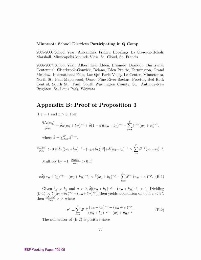
Minnesota School Districts Participating in Q Comp

2005-2006 School Year: Alexandria, Fridley, Hopkings, La Crescent-Hokah,Marshall, Minneapolis Mounds View, St. Cloud, St. Francis

2006-2007 School Year: Albert Lea, Alden, Brainerd, Brandon, Burnsville,Centennial, Clearbrook-Gonvick, Delano, Eden Prairie, Farmington, GrandMeadow, International Falls, Lac Qui Parle Valley Le Center, Minnetonka,North St. Paul-Maplewood, Osseo, Pine River-Backus, Proctor, Red RockCentral, South St. Paul, South Washington County, St. Anthony-NewBrighton, St. Louis Park, Wayzata

Appendix B: Proof of Proposition 3

If γ = 1 and ρ > 0, then

∂∆(w0)

∂w0

= δ̃π(w0 + bH)−ρ + δ̃(1− π)(w0 + bL)−ρ −T∑t=τ

δt−τ (w0 + vt)−ρ,

where δ̃ =∑Tt=τ δ

T−τ .

∂∆(w0)∂w0

> 0 if δ̃π[(w0+bH)−ρ−(w0+bL)−ρ]+δ̃(w0+bL)−ρ >T∑t=τ

δt−τ (w0+vt)−ρ.

Multiply by −1, ∂∆(w0)∂w0

> 0 if

πδ̃[(w0 + bL)−ρ − (w0 + bH)−ρ] < δ̃(w0 + bL)−ρ −T∑t=τ

δt−τ (w0 + vt)−ρ. (B-1)

Given bH > bL and ρ > 0, δ̃[(w0 + bL)−ρ − (w0 + bH)−ρ] > 0. Dividing(B-1) by δ̃[(w0 +bL)−ρ−(w0 +bH)−ρ], then yields a condition on π: if π < π∗,

then ∂∆(w0)∂w0

> 0, where

π∗ =T∑t=τ

δt−τ(w0 + bL)−ρ − (w0 + vt)

−ρ

(w0 + bL)−ρ − (w0 + bH)−ρ. (B-2)

The numerator of (B-2) is positive since

35


(w0 + bL)−ρ > (w0 + vt)−ρ,

and we assume bL < vt for all t. The denominator of (B-2) is also positiveby a similar argument. Hence π∗ > 0. In addition, the denominator of (B-2)is always larger than the numerator since bH > vt for all t. Hence π∗ < 1.QED

36


37

Table 1: Summary of Q Comp Plans

Mean Standard

Dev. N Performance Bonus Size Total 1912 653 24 Bonus/ (Minimum BA salary) 0.060 0.022 20 Bonus/ (BA step increase) 2.170 0.968 20 Bonus/ (MA step increase) 1.588 0.668 20

Performance Bonus Source FractionStandard

Error N Rubric and Peer Evaluation 0.689 0.058 24 Student Achievement (classroom) 0.140 0.033 Student Achievement (school) 0.171 0.033 Evaluation Required for Raise Yes 0.529 0.087 34 No 0.294 0.079 TBD 0.177 0.066

Notes: Step increase defined as the average salary increase over the first 10 years under the step and lanes salary schedule. Source: 2005-2006 salary schedules from Education Minnesota. Performance bonus data from district Q Comp proposals.


38

Table 2: Descriptive Statistics

Non Q Comp

Q Comp Approved

Mean Mean Difference in Means

(Std. Dev.) (Std. Dev.) (Std.

Error)

Teacher Characteristics

Avg. Teacher Age 41.823 41.556 0.282 (2.577) (2.562) (0.464)

Avg. Teacher Experience 16.413 15.811 0.602 (2.577) (2.925) (0.524)

Percent of Teachers Black 0.154 0.495 -0.342 (0.512) (0.243) (0.248)

Percent of Teachers Hispanic 0.198 0.437 -0.239 (0.032) (0.130) (0.134)

Percentage of Teachers Male 32.49 29.733 3.042 (7.065) (6.098) (1.115)

Percentage of Teachers w/ Masters Deg. 32.19 50.056 -17.879 (17.637) (17.009) (3.095)

Teacher Salary Characteristics

Starting Salary with Bachelors Deg.(1,000 $) 23.107 24.236 -1.129 (12.547) (12.589) (2.281)

Max. Salary with Bachelors Deg. (1,000 $) 34.825 39.775 -4.949 (19.386) (21.608) (3.877)

Max. Salary with Masters Deg. (1,000 $) 41.028 46.982 -5.953 (22.715) (25.274) (4.535)

Difference Between Max. and Min. 11.718 15.539 -3.821 Bachelors Deg. Salaries (1,000 $) (7.905) (10.306) (1.827)

Student Characteristics

Attendance Rate 94.862 94.834 -0.007

(2.819) (1.548) (0.313) Percentage of Students Black 1.52 5.735 -4.205

(0.213) (1.413) (1.429) Percentage of Students Hispanic 3.803 3.915 -0.111

(0.347) (0.702) (0.783) Perc. Free or Reduced Price Lunch 33.634 26.06 7.506

(14.234) (14.490) (2.623) Total Students (1,000) 2.013 6.334 -4.32

(0.246) (1.345) (1.367)


39

Table 2: Descriptive Statistic (con't)

Non Q Comp

Q Comp Approved

Mean Mean Difference in Means

(Std. Dev.) (Std. Dev.) (Std. Error)

Student Test Scores Percentage of Students Earning Level 5 Score in …

3rd Grade Mathematics 13.23 15.601 -2.371 (8.892) (8.222) (1.505) 3rd Grade Reading 16.319 19.903 -3.585 (8.364) (5.914) (1.128) 5th Grade Mathematics 14.602 20.024 -5.423 (8.477) (9.629) (1.725) 5th Grade Reading 23.129 29.336 -6.207 (9.286) (9.119) (1.656) Community/District Characteristics Percentage of Pop. with Bachelor Deg. 11.013 17.685 -6.63 (5.018) (9.265) (1.616) District Total Population (1,000) 11.478 40.827 -29.204 (24.687) (64.458) (11.150) Median Family Income (1,000 $) 48.017 58.9 -10.883 (0.604) (2.690) (2.757) Per Student Expenditure (1,000 $) 7.925 7.841 0.074 (1.158) (1.006) (0.185) Total Full Time Teachers 126.593 376.44 -249.847 (259.642) (491.643) (85.684) Student to Teacher Ratio 14.829 16.506 -1.63 (2.475) (1.874) (0.352)

Notes: 328 school districts used in analysis, 34 of which approved a Q Comp program by March 2007. Standard errors for difference in means calculated assuming unequal variances. Sources: 2004-2005 School District Data, 2004 Financial Data, and 2003 MCA test data from the Minnesota Department of Education and the NCES Common Core of Data.


40

Table 3: Relationship of Q Comp Approval to District Characteristics

Dependent Variable: Approval of Q Comp

(1) (2) (3) (4)

Percentage of Teachers w/ Masters Deg. 0.0041 0.0018

(0.0008)*** (0.0010)* Avg. Teacher Experience -0.0073 0.0076

(0.0062) (0.0053) Max. Salary with Bachelors Deg. 0.0117 0.0059

(1000 $) (0.0029)*** (0.0025)**

District Level Control Variables No No No Yes

N 328 328 328 328 Log Likelihood 94.9646 108.5503 100.6428 81.4161

Pseudo R-Squared 0.1307 0.0063 0.0787 0.2547

Notes: *significant at 10 percent level, **significant at 5 percent level, ***significant at 1 percent level. This Table reports marginal effects from a probit model where the marginal effects are reported at the mean of each variable. Standard errors in parentheses. Specifications with teacher salary data include a dummy variable for missing values. District Level Control Variables include percentage black teachers, percentage Hispanic teachers, percentage male teachers, student attendance rate, percentage of 5th grade student with level 5 in reading on assessment, percentage with reduced price lunch, percentage of black students, percentage of Hispanic students, student to teacher ratio, median family income in the district, percentage of population with bachelor degree, per student expenditures, and total students in district. Sources: 2004-2005 School District Data, 2004 Financial Data, and 2003 MCA Test Data from the Minnesota Department of Education and the NCES Common Core of Data.


41

Table 4: Teacher Evaluation Required for Salary Change

Evaluation Required? Yes No TBD N

Percent Teachers MA/PHD 53.92 42.66 49.24 34

(14.54) (19.56) (20.32) Max BA Salary 52.99 47.55 44.97 27

(8.28) (5.15) (5.99) Avg. Years Experience 15.21 16.79 16.37 34

(2.05) (4.08) (3.39) Percent Lv. 5

(Reading) 29.89 30.30 24.15 34 (9.92) (8.14) (7.19)

Observations 20 10 4 Notes: Sample means for Q Comp school districts reported with standard errors in parentheses. Determination of whether an evaluation is required for salary change is based on a school district’s Q Comp Approval Letter and correspondence with the Minnesota Department of Education. See Appendix details. Sources: 2004-2005 School District Data and 2003 MCA Test Data from the Minnesota Department of Education.


42

Figure 1: Average Salary Schedule for Minnesota Q Comp School Districts Prior to Q Comp

Source: 2006-2007 Salary Schedule Data (before Q Comp approval) from Education Minnesota. The figure uses 2006-2007 salary data obtained from the state teachers union, Education Minnesota. Schedules were available for 28 of the 34 Q Comp participating districts. These schedules reflect agreements made between school districts and the local teachers unions before Q Comp implementation.


43

Figure 2: Simulation: Relative Gains from Merit Pay by Base Pay

-4

-3.5

-3

-2.5

-2

-1.5

-1

-0.5

0

0.5

1

30 35 40 45 50

Rela

tive

Gain

s fr

om

Meri

t P

ay

Base Salary ($1000)

Notes: Relative Gains from Merit Pay is the relative proportional gains to merit: | Gains – Gains at Base Salary at 30,000| / | Gains at Base Salary of $30,000|. Sources: Simulation from parameters defined in the text.

Gamma = 0

Gamma = 1Risk Averse (Rho = 3)

Risk Neutral (Rho = 0)

Gamma = 0

Gamma = 1


44

Figure 3: Distribution across School Districts of Fraction of Teachers with Masters Degrees

Source: 2004-2005 School District Data from the Minnesota Department of Education.


The Institute for Education and Social Policy of the Steinhardt School of Culture, Education, and Human Development and Robert F. Wagner School of Public Service at NYU conducts non-partisan scientific research about U.S. education and related social issues. Our research, policy studies, evalu-ations, seminar series, and technical assistance inform and support policy makers, educators, parents and others in their efforts to improve public schooling. More information is available on our website at http://steinhardt.nyu.edu/iesp.

82 Washington Square East, 7th Floor New York, NY 10003 p 212.998.5880 f 212.995.4564

09-02 FRONT COVER - steinhardt.nyu.edu Working... · WORKING PAPER #09-05 April 2009....

Documents

Transcript of 09-02 FRONT COVER - steinhardt.nyu.edu Working... · WORKING PAPER #09-05 April 2009....