08 ELC4340 Spring13 Transmission Lines

8/9/2019 08 ELC4340 Spring13 Transmission Lines

http://slidepdf.com/reader/full/08-elc4340-spring13-transmission-lines 1/32

_08_ELC4340_Spring13_Transmission_Lines.doc, V130228

of 32

Transmission Lines

Inductance and capacitance calculations for transmission lines. GMR, GMD, L, and C matrices,

effect of ground conductivity. Underground cables.

1. Equivalent Circuit for Transmission Lines (Including Overhead and Underground)

The power system model for transmission lines is developed from the conventional distributed

parameter model, shown in Figure 1.

+

-

v

R/2 L/2

G C

R/2 L/2

i --->

<--- i

+

-

v + dv

i + di --->

<--- i + di

R, L, G, C per unit length

< >dz

Figure 1. Distributed Parameter Model for Transmission Line

Once the values for distributed parameters resistance R, inductance L, conductance G, and

capacitance are known (units given in per unit length), then either "long line" or "short line"

models can be used, depending on the electrical length of the line.

Assuming for the moment that R, L, G, and C are known, the relationship between voltage and

current on the line may be determined by writing Kirchhoff's voltage law (KVL) around the outer

loop in Figure 1, and by writing Kirchhoff's current law (KCL) at the right-hand node.

KVL yields

02222

t

i Ldz i

Rdz dvv

t

i Ldz i

Rdz v

.

This yields the change in voltage per unit length, or

t

i L Ri

z

v

,

which in phasor form is

I L j R z

V ~~

.




of 32

KCL at the right-hand node yields

0

t

dvvCdz dvvGdz diii

.

If dv is small, then the above formula can be approximated as

t

vCdz vGdz di

, or

t

vC Gv

z

i

, which in phasor form is

V C jG z

I ~~

.

Taking the partial derivative of the voltage phasor equation with respect to z yields

z

I

L j R z

V

~~

2

2

.

Combining the two above equations yields

V V C jG L j R z

V ~~~

2

2

2

, where jC jG L j R , and

where , , and are the propagation, attenuation, and phase constants, respectively.

The solution for V ~

is

z z Be Ae z V )(~ .

A similar procedure for solving I ~

yields

o

z z

Z

Be Ae z I

)(~

,

where the characteristic or "surge" impedance o Z is defined as

C jG L j R Z o

.

Constants A and B must be found from the boundary conditions of the problem. This is usually

accomplished by considering the terminal conditions of a transmission line segment that is d

meters long, as shown in Figure 2.




of 32

d< >

+

-

+

-

Vs Vr

Is ---> Ir --->

<--- Is<--- Ir

Sending End Receiving End

z = 0z = -d

Ysr

Ys Yr

o RS

Z

d

Y Y

2tanh

, d Z

Y o

SR sinh

1 ,

C jG

L j R Z o

, C jG L j R

R, L, G, C per unit length

Figure 3. Pi Equivalent Circuit Model for Distributed Parameter Transmission Line

Shunt conductance G is usually neglected in overhead lines, but it is not negligible in

underground cables.

For electrically "short" overhead transmission lines, the hyperbolic pi equivalent model

simplifies to a familiar form. Electrically short implies that d < 0.05 , where wavelength

Hz f

sm

r /103 8

= 5000 km @ 60 Hz, or 6000 km @ 50 Hz. Therefore, electrically short

overhead lines have d < 250 km @ 60 Hz, and d < 300 km @ 50 Hz. For underground cables,

the corresponding distances are less since cables have somewhat higher relative permittivities(i.e. 5.2r ).

Substituting small values of d into the hyperbolic equations, and assuming that the line losses

are negligible so that G = R = 0, yields

2

Cd jY Y RS

, and

Ld jY SR

1 .

Then, including the series resistance yields the conventional "short" line model shown in Figure

4, where half of the capacitance of the line is lumped on each end.




of 32

< >d

Cd

2

Cd

2

Rd Ld

R, L, C per unit length

Figure 4. Standard Short Line Pi Equivalent Model for a Transmission Line

2. Capacitance of Overhead Transmission Lines

Overhead transmission lines consist of wires that are parallel to the surface of the Earth. To

determine the capacitance of a transmission line, first consider the capacitance of a single wire

over the Earth. Wires over the Earth are typically modeled as line charges l Coulombs permeter of length, and the relationship between the applied voltage and the line charge is the

capacitance.

A line charge in space has a radially outward electric field described as

r o

l ar

q E ˆ2

Volts per meter .

This electric field causes a voltage drop between two points at distances r = a and r = b away

from the line charge. The voltage is found by integrating electric field, or

a

bqar E V

o

l r

br

ar

ab ln2

ˆ

V.

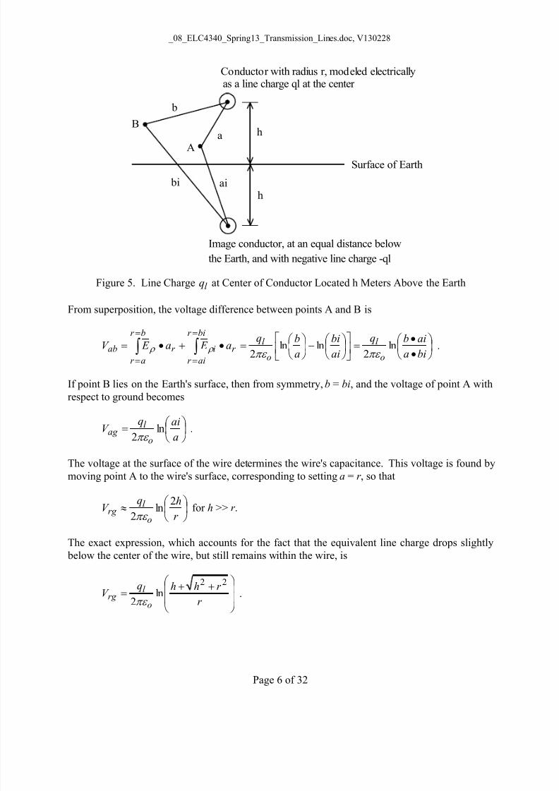
If the wire is above the Earth, it is customary to treat the Earth's surface as a perfect conducting

plane, which can be modeled as an equivalent image line charge l q lying at an equal distance

below the surface, as shown in Figure 5.




of 32

Surface of Earth

h

a

b

ai bi

A

Bh

Conductor with radius r, modeled electricallyas a line charge ql at the center

Image conductor, at an equal distance below

the Earth, and with negative line charge -ql

Figure 5. Line Charge l q at Center of Conductor Located h Meters Above the Earth

From superposition, the voltage difference between points A and B is

bia

aibq

ai

bi

a

bqa E a E V

o

l

o

l r

bir

air

ir

br

ar

ab ln2

lnln2

ˆˆ

.

If point B lies on the Earth's surface, then from symmetry, b = bi, and the voltage of point A with

respect to ground becomes

a

aiqV

o

l ag ln2

.

The voltage at the surface of the wire determines the wire's capacitance. This voltage is found by

moving point A to the wire's surface, corresponding to setting a = r , so that

r

hqV

o

l rg

2ln

2 for h >> r .

The exact expression, which accounts for the fact that the equivalent line charge drops slightly

below the center of the wire, but still remains within the wire, is

r

r hhqV

o

l rg

22

ln2

.




of 32

The capacitance of the wire is defined asrg

l

V

qC which, using the approximate voltage formula

above, becomes

r

hC o

2ln

2

Farads per meter of length.

When several conductors are present, then the capacitance of the configuration is given in matrix

form. Consider phase a-b-c wires above the Earth, as shown in Figure 6.

a

ai

b

bi

c

ci

Daai

Dabi

Daci

Dab

Dac

Surface of Earth

Three Conductors Represented by Their Equivalent Line Charges

Images

Conductor radii ra, rb, rc

Figure 6. Three Conductors Above the Earth

Superposing the contributions from all three line charges and their images, the voltage at the

surface of conductor a is given by

ac

acic

ab

abib

a

aaia

oag

D

Dq

D

Dq

r

DqV lnlnln

2

1

.

The voltages for all three conductors can be written in generalized matrix form as

c

b

a

cccbca

bcbbba

acabaa

ocg

bg

ag

q

q

q

p p p

p p p

p p p

V

V

V

2

1 , or abcabc

oabc Q P V

2

1 ,

where




of 32

a

aaiaa

r

D p ln ,

ab

abiab

D

D p ln , etc., and

ar is the radius of conductor a, etc.,

aai D is the distance from conductor a to its own image (i.e. twice the height of

conductor a above ground),

ab D is the distance from conductor a to conductor b,

baiabi D D is the distance between conductor a and the image of conductor b (which

is the same as the distance between conductor b and the image of

conductor a), etc. Therefore, P is a symmetric matrix.

A Matrix Approach for Finding C

From the definition of capacitance, CV Q , then the capacitance matrix can be obtained via

inversion, or

12 abcoabc P C .

If ground wires are present, the dimension of the problem increases by the number of ground

wires. For example, in a three-phase system with two ground wires, the dimension of the P

matrix is 5 x 5. However, given the fact that the line-to-ground voltage of the ground wires is

zero, equivalent 3 x 3 P and C matrices can be found by using matrix partitioning and a process

known as Kron reduction. First, write the V = PQ equation as follows:

w

v

c

b

a

vwabcvw

vwabcabc

o

wg

vg

cg

bg

ag

q

q

q

q

q

P P

P P

V

V

V

V

V

)2x2(|)3x2(

)2x3(|)3x3(

2

1

0

0 ,

,

,

or

vw

abc

vwabcvw

vwabcabc

ovw

abc

Q

Q

P P

P P

V

V

,

,

2

1

,

where subscripts v and w refer to ground wires w and v, and where the individual P matrices are

formed as before. Since the ground wires have zero potential, then




of 32

The diagonal terms of C are positive, and the off-diagonal terms are negative. a va b cC has the

special symmetric form for diagonalization into 012 components, which yields

M S

M S

M S avg

C C C C

C C

C 00

00

002

012 .

The Approximate Formulas for 012 Capacitances

Asymmetries in transmission lines prevent the P and C matrices from having the special form

that perfect diagonalization into decoupled positive, negative, and zero sequence impedances.

Transposition of conductors can be used to nearly achieve the special symmetric form and,

hence, improve the level of decoupling. Conductors are transposed so that each one occupies

each phase position for one-third of the lines total distance. An example is given below in Figure

7, where the radii of all three phases are assumed to be identical.

a b c a cthen then

then then

bthen

b a c

b c a c a b c b a

where each configuration occupies one-sixth of the total distance

Figure 7. Transposition of A-B-C Phase Conductors

For this mode of construction, the average P matrix (or Kron reduced P matrix if ground wires

are present) has the following form:

cc

acaa

bcabbb

bb

bccc

abacaa

cc

bcbb

acabaaavg

abc

p

p p

p p p

p

p p

p p p

p

p p

p p p

P 6

1

6

1

6

1

aa

abbb

acbccc

aa

accc

abbcbb

bb

abaa

bcaccc

p p p

p p p

p p p

p p p

p p p

p p p

6

1

6

1

,

where the individual p terms are described previously. Note that these individual P matrices are

symmetric, since baabbaab p p D D , , etc. Since the sum of natural logarithms is the same

as the logarithm of the product, P becomes




of 32

S M M

M S M

M M S avg

abc

p p p

p p p

p p p

P ,

where

3

3

ln3 cba

ccibbiaaiccbbaa s

r r r

D D D P P P p

,

and

3

3

ln3 bcacab

bciaciabibcacab M

D D D

D D D P P P p

.

Since avg abc P has the special property for diagonalization in symmetrical components, then

transforming it yields

M S

M S

M S avg

p p

p p

p p

p

p

p

P

00

00

002

00

00

00

2

1

0

012 .

The pos/neg sequence values are

33

33

3

3

3

3

lnlnlnbciaciabicba

bcacabccibbiaaibcacabbciaciabi

cbaccibbiaai M s

D D Dr r r

D D D D D D

D D D

D D D

r r r

D D D p p .

When the a-b-c conductors are closer to each other than they are to the ground, then

bciaciabiccibbiaai D D D D D D ,

yielding the conventional approximation

2,1

2,1

3

3

21 lnlnGMR

GMD

r r r

D D D p p p p

cba

bcacab M S ,

where 2,1GMD and 2,1GMR are the geometric mean distance (between conductors) and

geometric mean radius, respectively, for both positive and negative sequences.

The zero sequence value is




of 32

3

3

3

3

0 ln2ln2bcacab

bciaciabi

cba

ccibbiaai M s

D D D

D D D

r r r

D D D p p p

3

2

2

ln

bcacabba

bciaciabiccibbiaai

D D Dr r r

D D D D D D .

Expanding yields

9

2

2

0 ln3

bcacabba

bciaciabiccibbiaai

D D Dr r r

D D D D D D p

9ln3cbcababcacabba

cbicaibaibciaciabiccibbiaai

D D D D D Dr r r

D D D D D D D D D ,

or

0

00 ln3

GMR

GMD p ,

where

90 cbicaibaibciaciabiccibbiaai D D D D D D D D DGMD ,

90 cbcababcacabcba D D D D D Dr r r GMR .

Invertingavg

P 012 and multiplying by o 2 yields the corresponding 012 capacitance matrix

M S

M S

M S

ooavg

p p

p p

p p

p

p

p

C

C

C

C

100

01

0

002

1

2

100

01

0

001

2

00

00

00

2

1

0

2

1

0

012

Thus, the pos/neg sequence capacitance is

2,1

2,121

ln

22

GMR

GMD p pC C o

M S

o

Farads per meter,




of 32

and the zero sequence capacitance is

o

o

M S

o

GMR

GMD p pC

00

ln

2

3

1

2

2

Farads per meter,

which is one-third that of the entire a-b-c bundle by because it represents the charge due to only

one phase of the abc bundle.

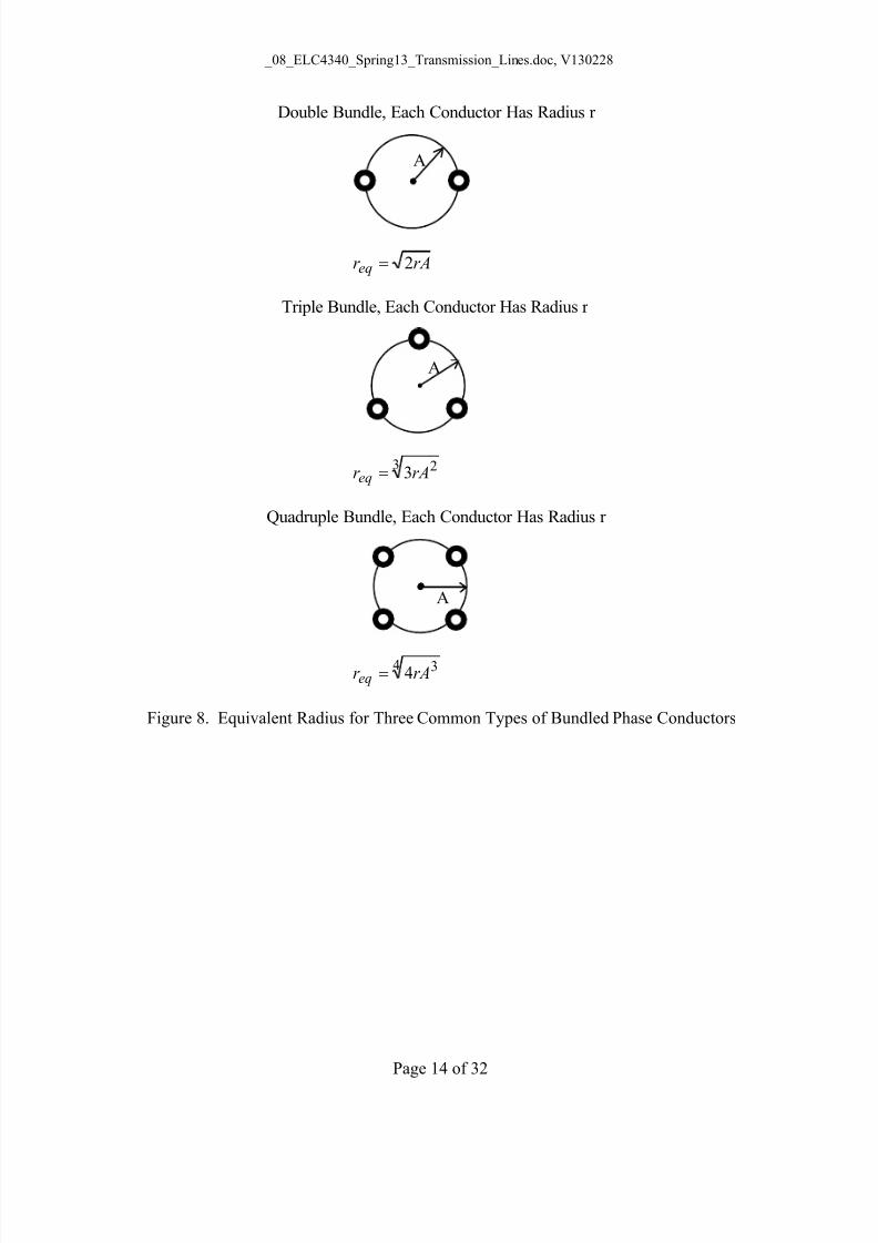
Bundled Phase Conductors

If each phase consists of a symmetric bundle of N identical individual conductors, an equivalent

radius can be computed by assuming that the total line charge on the phase divides equally

among the N individual conductors. The equivalent radius is

N N

eq NrAr

11

,

where r is the radius of the individual conductors, and A is the bundle radius of the symmetric set

of conductors. Three common examples are shown below in Figure 8.




of 32

Double Bundle, Each Conductor Has Radius r

A

rAr eq 2

Triple Bundle, Each Conductor Has Radius r

A

3 23rAr eq

Quadruple Bundle, Each Conductor Has Radius r

A

4 34rAr eq

Figure 8. Equivalent Radius for Three Common Types of Bundled Phase Conductors




of 32

3. Inductance

The magnetic field intensity produced by a long, straight current carrying conductor is given by

Ampere's Circuital Law to be

r

I H

2 Amperes per meter,

where the direction of H is given by the right-hand rule.

Magnetic flux density is related to magnetic field intensity by permeability as follows:

H B Webers per square meter,

and the amount of magnetic flux passing through a surface is

sd B Webers,

where the permeability of free space is 7104 o .

Two Paral lel Wi res in Space

Now, consider a two-wire circuit that carries current I, as shown in Figure 9.

I I

Two current-carying wires with radii r

D< >

Figure 9. A Circuit Formed by Two Long Parallel Conductors

The amount of flux linking the circuit (i.e. passes between the two wires) is found to be

r

r D I dx

x

I dx

x

I or D

r

or D

r

o

ln22

Henrys per meter length.

From the definition of inductance,

I

N L

,




of 32

where in this case N = 1, and where N >> r , the inductance of the two-wire pair becomes

r

D L o ln


A round wire also has an internal inductance, which is separate from the external inductanceshown above. The internal inductance is shown in electromagnetics texts to be

8

int int L Henrys per meter length.

For most current-carrying conductors, oint so that int L = 0.05µH/m. Therefore, the total

inductance of the two-wire circuit is the external inductance plus twice the internal inductance of

each wire (i.e. current travels down and back), so that

4

14

1

lnlnln41ln

82ln

re

Der

Dr

Dr

D L oooootot

.

It is customary to define an effective radius

r rer eff 7788.04

1

,

and to write the total inductance in terms of it as

eff

otot

r D L ln


Wire Parallel to Earth ’s Surface

For a single wire of radius r , located at height h above the Earth, the effect of the Earth can be

described by an image conductor, as it was for capacitance calculations. For perfectly

conducting earth, the image conductor is located h meters below the surface, as shown in Figure

10.




of 32

Surface of Earth

h

h

Conductor of radius r, carrying current I

Note, the image

flux exists only

above the Earth

Image conductor, at an equal distance below the Earth

Figure 10. Current-Carrying Conductor Above the Earth

The total flux linking the circuit is that which passes between the conductor and the surface of

the Earth. Summing the contribution of the conductor and its image yields

r

r h I

rh

r hh I

x

dx

x

dx I ooh

r

r h

h

o 2ln2

2ln22

2

.

For 2h r , a good approximation is

r

h I o 2ln2

Webers per meter length,

so that the external inductance per meter length of the circuit becomes

r

h L o

ext 2ln2


The total inductance is then the external inductance plus the internal inductance of one wire, or

4

1

2ln24

12ln28

2ln2

re

h

r

h

r

h L oooo

tot

,

or, using the effective radius definition from before,

eff

otot

r

h L 2ln2





of 32

Bundled Conductors

The bundled conductor equivalent radii presented earlier apply for inductance as well as for

capacitance. The question now is “what is the internal inductance of a bundle?” For N bundled

conductors, the net internal inductance of a phase per meter must decrease as

N

1 because the

internal inductances are in parallel. Considering a bundle over the Earth, then

N

eq

o

eq

o

eq

oo

eq

otot

er

he

N r

h

N r

h

N r

h L

4

14

12

ln2

ln12

ln24

12ln28

2ln2

.

Factoring in the expression for the equivalent bundle radius eqr yields

N N eff

N N N N N N

eq A Nr A Nree NrAer

11

1

14

1

4

1114

1

Thus, eff r remains 4

1

re , no matter how many conductors are in the bundle.

The Thr ee-Phase Case

For situations with multiples wires above the Earth, a matrix approach is needed. Consider thecapacitance example given in Figure 6, except this time compute the external inductances, rather

than capacitances. As far as the voltage (with respect to ground) of one of the a-b-c phases is

concerned, the important flux is that which passes between the conductor and the Earth's surface.

For example, the flux "linking" phase a will be produced by six currents: phase a current and its

image, phase b current and its image, and phase c current and its image, and so on. Figure 11 is

useful in visualizing the contribution of flux “linking” phase a that is caused by the current in

phase b (and its image).




of 32

a

ai

b

bi

Dab

D bg

D bg Dabi

g

Figure 11. Flux Linking Phase a Due to Current in Phase b and Phase b Image




of 32

The linkage flux is

a (due to b I and b I image) =ab

abibo

bg

abibo

ab

bg bo

D

D I

D

D I

D

D I ln2

ln2

ln2

.

Considering all phases, and applying superposition, yields the total flux

ac

acico

ab

abibo

a

aaiaoa

D

D I

D

D I

r

D I ln2

ln2

ln2

.

Note that aai D corresponds to 2h in Figure 10. Performing the same analysis for all three

phases, and recognizing that LI N , where N = 1 in this problem, then the inductance matrix

is developed using

c

b

a

c

cci

cb

cbi

ca

cai

bc

bci

b

bbi

ba

bai

ac

aci

ab

abi

a

aai

o

c

b

a

I

I

I

r

D

D

D

D

D

D

D

r

D

D

D D

D

D

D

r

D

lnlnln

lnlnln

lnlnln

2

, or abcabcabc I L .

A comparison to the capacitance matrix derivation shows that the same matrix of natural

logarithms is used in both cases, and that

11222

abcoabco

o

abc

o

abc C C P L

.

This implies that the product of the L and C matrices is a diagonal matrix with o on the

diagonal, providing that the Earth is assumed to be a perfect conductor and that the internal

inductances of the wires are ignored.

If the circuit has ground wires, then the dimension of L increases accordingly. Recognizing that

the flux linking the ground wires is zero (because their voltages are zero), then L can be Kron

reduced to yield an equivalent 3 x 3 matrix 'abc L .

To include the internal inductance of the wires, replace actual conductor radius r with eff r .

Computing 012 Inductances fr om Matri ces

Once the 3 x 3 'abc L matrix is found, 012 inductances can be determined by averaging the

diagonal terms, and averaging the off-diagonal terms, of 'abc L to produce




of 32

S M M

S S M

M M S avg abc

L L L

L L L

L L L

L ,

so that

M S

M S

M S avg

L L

L L

L L

L

00

00

002

012 .

The Approximate Formulas for 012 Inductancess

Because of the similarity to the capacitance problem, the same rules for eliminating ground

wires, for transposition, and for bundling conductors apply. Likewise, approximate formulas for

the positive, negative, and zero sequence inductances can be developed, and these formulas are

2,1

2,121 ln2 GMR

GMD L L o

,

and

0

00 ln23

GMR

GMD L o

.

It is important to note that the GMD and GMR terms for inductance differ from those of

capacitance in two ways:

1. GMR calculations for inductance calculations should be made with 4

1

rer eff .

2. GMD distances for inductance calculations should include the equivalent complex depth for

modeling finite conductivity earth (explained in the next section). This effect is ignored in

capacitance calculations because the surface of the Earth is nominally at zero potential.

Modeling Imperf ect Earth

The effect of the Earth's non-infinite conductivity should be included when computinginductances, especially zero sequence inductances. (Note - positive and negative sequences are

relatively immune to Earth conductivity.) Because the Earth is not a perfect conductor, the

image current does not actually flow on the surface of the Earth, but rather through a cross-

section. The higher the conductivity, the narrower the cross-section.




of 32

It is reasonable to assume that the return current is one skin depth δ below the surface of the

Earth, where f o

2

meters. Typically, resistivity is assumed to be 100Ω-m. For

100Ω-m and 60Hz, δ = 459m. Usually δ is so large that the actual height of the conductors

makes no difference in the calculations, so that the distances from conductors to the images is

assumed to be δ. However, for cases with low resistivity or high frequency, one should limit

delta to not be less than GMD computed with perfect Earth images.

#1 #2

#3

#1’ #2’

#3’ Images

Practice Area




of 32

4. Electric Field at Surface of Overhead Conductors

Ignoring all other charges, the electric field at a conductor’s surface can be approximated by

r

q E

o

r

2

,

where r is the radius. For overhead conductors, this is a reasonable approximation because the

neighboring line charges are relatively far away. It is always important to keep the peak electric

field at a conductor’s surface below 30kV/cm to avoid excessive corono losses.

Going beyond the above approximation, the Markt-Mengele method provides a detailed

procedure for calculating the maximum peak subconductor surface electric field intensity for

three-phase lines with identical phase bundles. Each bundle has N symmetric subconductors of

radius r . The bundle radius is A. The procedure is

1.

Treat each phase bundle as a single conductor with equivalent radius

N N eq NrAr /11 .

2. Find the C(N x N) matrix, including ground wires, using average conductor heights above

ground. Kron reduce C(N x N) to C(3 x 3). Select the phase bundle that will have the

greatest peak line charge value ( lpeak q ) during a 60Hz cycle by successively placing

maximum line-to-ground voltage V max on one phase, and – V max/2 on each of the other

two phases. Usually, the phase with the largest diagonal term in C(3 by 3) will have the

greatest lpeak q .

3. Assuming equal charge division on the phase bundle identified in Step 2, ignore

equivalent line charge displacement, and calculate the average peak subconductor surface

electric field intensity using

r N

q E

o

lpeak peak avg

2

1,

4. Take into account equivalent line charge displacement, and calculate the maximum peak

subconductor surface electric field intensity using

A

r N E E peak avg peak )1(1,max, .

5. Resistance and Conductance

The resistance of conductors is frequency dependent because of the resistive skin effect. Usually,

however, this phenomenon is small for 50 - 60 Hz. Conductor resistances are readily obtained




of 32

from tables, in the proper units of ohms per meter length, and these values, added to the

equivalent-Earth resistances from the previous section, to yield the R used in the transmission

line model.

Conductance G is very small for overhead transmission lines and can be ignored.

6. Underground Cables

Underground cables are transmission lines, and the model previously presented applies.

Capacitance C tends to be much larger than for overhead lines, and conductance G should not be

ignored.

For single-phase and three-phase cables, the capacitances and inductances per phase per meter

length are

a

bC r o

ln

2 Farads per meter length,

and

a

b L o ln2

Henrys per meter length,

where b and a are the outer and inner radii of the coaxial cylinders. In power cables,a

b is

typically e (i.e., 2.7183) so that the voltage rating is maximized for a given diameter.

For most dielectrics, relative permittivity 5.20.2 r . For three-phase situations, it is

common to assume that the positive, negative, and zero sequence inductances and capacitances

equal the above expressions. If the conductivity of the dielectric is known, conductance G can be

calculated using

C G Mhos per meter length.




of 32

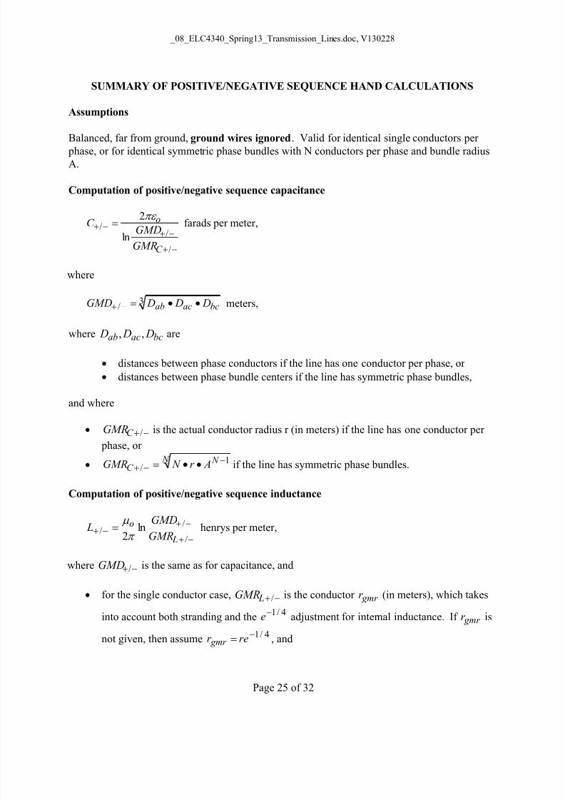
SUMMARY OF POSITIVE/NEGATIVE SEQUENCE HAND CALCULATIONS

Assumptions

Balanced, far from ground, ground wires ignored. Valid for identical single conductors per phase, or for identical symmetric phase bundles with N conductors per phase and bundle radius

A.

Computation of positive/negative sequence capacitance

/

//

ln

2

C

o

GMR

GMDC

farads per meter,

where

3/ bcacab D D DGMD meters,

where bcacab D D D ,, are

distances between phase conductors if the line has one conductor per phase, or

distances between phase bundle centers if the line has symmetric phase bundles,

and where

/C GMR is the actual conductor radius r (in meters) if the line has one conductor per

phase, or

N N C Ar N GMR 1/

if the line has symmetric phase bundles.

Computation of positive/negative sequence inductance

/

// ln2 L

o

GMR

GMD L

henrys per meter,

where /GMD is the same as for capacitance, and

for the single conductor case, / LGMR is the conductor gmr r (in meters), which takes

into account both stranding and the4/1e adjustment for internal inductance. If gmr r is

not given, then assume 4/1 rer gmr , and




of 32

for bundled conductors, N N gmr L Ar N GMR 1

/

if the line has symmetric phase

bundles.

Computation of positive/negative sequence resistance

R is the 60Hz resistance of one conductor if the line has one conductor per phase. If the line has

symmetric phase bundles, then divide the one-conductor resistance by N.

Some commonly-used symmetric phase bundle configurations

SUMMARY OF ZERO SEQUENCE HAND CALCULATIONS

Assumptions

Ground wires are ignored. The a-b-c phases are treated as one bundle. If individual phase

conductors are bundled, they are treated as single conductors using the bundle radius method.

For capacitance, the Earth is treated as a perfect conductor. For inductance and resistance, the

Earth is assumed to have uniform resistivity . Conductor sag is taken into consideration, and a

good assumption for doing this is to use an average conductor height equal to (1/3 the conductor

height above ground at the tower, plus 2/3 the conductor height above ground at the maximum

sag point).

The zero sequence excitation mode is shown below, along with an illustration of the relationship

between bundle C and L and zero sequence C and L. Since the bundle current is actually 3Io, the

zero sequence resistance and inductance are three times that of the bundle, and the zero sequence

capacitance is one-third that of the bundle.

A A A

N = 2 N = 3 N = 4




of 32

Computation of zero sequence capacitance

0

00

ln

2

3

1

C

C

o

GMR

GMDC

farads per meter,

where 0C GMD is the average height (with sag factored in) of the a-b-c bundle above perfect

Earth. 0C GMD is computed using

9222

0 ibciaciabiccibbiaaC D D D D D DGMD meters,

where iaa D is the distance from a to a-image, iab

D is the distance from a to b-image, and so

forth. The Earth is assumed to be a perfect conductor, so that the images are the same distance

below the Earth as are the conductors above the Earth. Also,

92223

/0 bcacabC C D D DGMRGMR meters,

where /C GMR , ab D , ac D , and bc D were described previously.

+

Vo

–

Io →

Io →

Io → 3Io →

C bundle

+

Vo

–

Io →

Io →

Io → 3Io →

3Io ↓

L bundle

+

Vo

–

Io →

Io →

Io → 3Io →

Co Co Co

Io →

+

Vo

–

Io →

Io → 3Io →

3Io ↓ Lo

Lo

Lo




of 32

Computation of zero sequence inductance

00 ln23

L

o

GMR L

Henrys per meter, 0C GMD

where skin depth f o

2

meters. Resistivity ρ = 100 ohm-meter is commonly used. For

poor soils, ρ = 1000 ohm-meter is commonly used. For 60 Hz, and ρ = 100 ohm-meter, skin

depth δ is 459 meters. To cover situations with low resistivity, use 0C GMD (from the previous

page) as a lower limit for δ

The geometric mean bundle radius is computed using

92223

/0 bcacab L L D D DGMRGMR meters,

where / LGMR , ab D , ac D , and bc D were shown previously.

Computation of zero sequence resistance

There are two components of zero sequence line resistance. First, the equivalent conductor

resistance is the 60Hz resistance of one conductor if the line has one conductor per phase. If the

line has symmetric phase bundles with N conductors per bundle, then divide the one-conductor

resistance by N.

Second, the effect of resistive earth is included by adding the following term to the conductor

resistance:

f 710869.93 ohms per meter (see Bergen),

where the multiplier of three is needed to take into account the fact that all three zero sequence

currents flow through the Earth.

As a general rule,

/C usually works out to be about 12 picoF per meter,

/ L works out to be about 1 microH per meter (including internal inductance).

0C is usually about 6 picoF per meter.




of 32

0 L is usually about 2 microH per meter if the line has ground wires and typical Earth

resistivity, or about 3 microH per meter for lines without ground wires or poor earth

resistivity.

The velocity of propagation, LC

1, is approximately the speed of light (3 x 10

8 m/s) for positive

and negative sequences, and about 0.8 times that for zero sequence.




of 32

5.7 m

4.4 m7.6 m

8.5 m

22.9 m at

tower, andsags down 10

m at mid-

span to 12.9

m.

7.6 m

7.8 m

Tower Base

345kV Double-Circuit Transmission Line

Scale: 1 cm = 2 m

Double conductor phase bundles, bundle radius = 22.9 cm, conductor radius = 1.41 cm, conductor

resistance = 0.0728 Ω/km

Single-conductor ground wires, conductor radius = 0.56 cm, conductor resistance = 2.87 Ω/km




of 32

5 m

10 m

33 m

Tower Base

500kV Single-Circuit Transmission Line

Scale: 1 cm = 2 m

Triple conductor phase bundles, bundle radius = 20 cm, conductor radius = 1.5 cm, conductor resistance =

0.05 Ω/km

Single-conductor ground wires, conductor radius = 0.6 cm, conductor resistance = 3.0 Ω/km

10 m

5 m

39 m

Conductors

sag down 10

m at mid-span

30 m

Earth resistivity ρ = 100 Ω-m




Practice Problem.

Use the left-hand circuit of the 345kV line geometry given two pages back. Determine the L, C,

R line parameters, per unit length, for positive/negative and zero sequence.

Now, focus on a balanced three-phase case, where only positive sequence is important, and work

the following problem using your L, C, R positive sequence line parameters:

For a 200km long segment, determine the P’s, Q’s, I’s, VR , and δR for switch open and

switch closed cases. The generator voltage phase angle is zero.

R jωL

jωC/2

1

jωC/2

1+

200kVrms

− 400Ω

P1 + jQ1

I1

QC1

produced

P2 + jQ2

I2

QL

absorbed

QC2

produced

+

VR / δR

−

08 ELC4340 Spring13 Transmission Lines

Documents

Transcript of 08 ELC4340 Spring13 Transmission Lines