06EC44-Signals and System –Session9-2009• and System –Chapter 6-2009• Krupa Rasane(KLE) Page...
24
06EC44-Signals and System –Chapter 6-2009• Krupa Rasane(KLE) Page 1 Chapter 6.1 FT representation of continuous periodic pulses To use Fourier methods to analyse interaction between continuous times and discrete-time signals, we need a bridge between Fourier representation for different signal classes FT representation of periodic signals Consider a continuous-time signal x(t) with a fundamental period equal to „To‟. This signal can be represented using exponential fourier series as We know that If we represent the transform in a periodic way we get Example 1 Show that the FT of a Dirac comb is also Dirac comb. Soln: A periodic impulse train is known as Dirac comb Example 1 • The Complex Fourier Coefficient is given by • The FT of x(t) is given by Example2 Find the FT, of the periodic signal x(t) and sketch the magnitude spectrum and the phase spectrum Soln: Comparing Eqn 1 with the FS synthesis eqn
Transcript of 06EC44-Signals and System –Session9-2009• and System –Chapter 6-2009• Krupa Rasane(KLE) Page...
06EC44-Signals and System –Chapter 6-2009•
Krupa Rasane(KLE) Page 1
Chapter 6.1
FT representation of continuous periodic pulses
To use Fourier methods to analyse interaction between continuous times and
discrete-time signals, we need a bridge between Fourier representation for
different signal classes
FT representation of periodic signals
Consider a continuous-time signal x(t) with a fundamental period equal to „To‟.
This signal can be represented using exponential fourier series as
We know that
If we represent the transform in a periodic way we get
Example 1
Show that the FT of a Dirac comb is also Dirac comb.
Soln: A periodic impulse train is known as Dirac comb
Example 1 • The Complex Fourier Coefficient is given by
• The FT of x(t) is given by
Example2
Find the FT, of the periodic signal x(t) and sketch the magnitude
spectrum and the phase spectrum
Soln:
Comparing Eqn 1 with the FS synthesis eqn

06EC44-Signals and System –Chapter 6-2009•
Krupa Rasane(KLE) Page 2
We get, X(0)=3, X(1)=1, X(-1)=1, and X(k)=0 for all other k.
Using the FT of a periodic signal x(t) is given by
Expanding the above Eqn
Substituting the coefficient values, we get
Fourier Transform of everlasting sinusoidal cosωot
FT FOR PERIODIC SIGNALS
For analysing Discrete time periodic and a periodic signals DTFT is used.
As in continuous time case, DT periodic signals can be incorporated within the
framework of the DTFT, by interpreting the transform of periodic signal as an
impulse train in the frequency domain
• Fourier Transform from Fourier series

06EC44-Signals and System –Chapter 6-2009•
Krupa Rasane(KLE) Page 3
Fourier Transform from Fourier series
In order to check the validity of the above expression let us use the synthesys
equation.
4.6.2 Fourier Transform from Fourier series
Note that any interval of length 2π includes exactly one pulse in the above
analysis eqn. Hence if the integral interval is chosen includes one pulse
located at ωo+2πr, then
Now consider a periodic sequence x[n] with period N its DTFS representation
is
So that the FS can be directly constructed from its coefficient.
To verify the above equation is correct note that x[n] in the above is a linear
combination of and thus must be a combination of transforms
In this case, the Fourier transform is
So that the FS can be directly constructed from its coefficient. To verify the above
equation is correct note that x[n] in the above is a linear combination of and thus must
be a combination of transforms Fourier Transform from Fourier series

06EC44-Signals and System –Chapter 6-2009•
Krupa Rasane(KLE) Page 4
Suppose we chose the summation of interval as k=0,1……N, so that
Hence x[n] is a linear combination of signals as initial x[n]. With ω0 =0,2π/N,
4π/N,……. (N-1)2π/N. The waveforms are depicted as
Example 1:
Consider the periodic signal
06EC44-Signals and System –Chapter 6-2009•
Krupa Rasane(KLE) Page 5
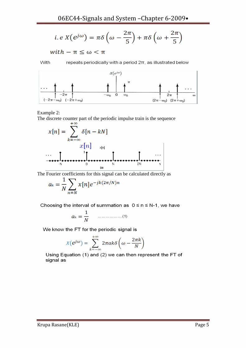
Example 2:
The discrete counter part of the periodic impulse train is the sequence
The Fourier coefficients for this signal can be calculated directly as
06EC44-Signals and System –Chapter 6-2009•
Krupa Rasane(KLE) Page 6
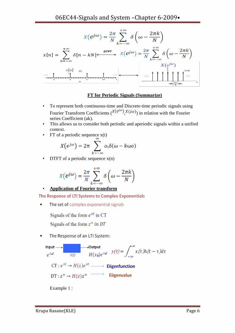
FT for Periodic Signals (Summarize)
• To represent both continuous-time and Discrete-time periodic signals using
Fourier Transform Coefficients ( , ) in relation with the Fourier
series Coefficient (ak).
• This allows us to consider both periodic and aperiodic signals within a unified
context.
• FT of a periodic sequence x(t)
• DTFT of a periodic sequence x(n)
• Application of Fourier transform
Example 1 :
06EC44-Signals and System –Chapter 6-2009•
Krupa Rasane(KLE) Page 7
As an illustration, consider an LTI system for which the input x(t) and output
y(t) are related by a time shift of 3, i.e y(t)=x(t-3). If the input to this system is
the complex exponential signal x(t) = ej2t
• Soln:
The impulse response is
Example 1.b
Consider the input signal x(t)=cos(4t)+cos(7t). Then, if as in example 1, y(t)=x(t-3),
then .
Expanding x(t), using Euler‟s relation
Representing in the above as the LTI System, we get the output as
Fourier Series and LTI System
• Fourier series representation can be used to construct any periodic signals in
discrete as well as continuous-time signals of practical importance.
• We have also seen the response of an LTI system to a linear combination of
complex exponentials taking a simple form.
• Now, let us see how Fourier representation is used to analyze the response of
LTI System.
Consider the CTFS synthesis equation for x(t) given by
Suppose we apply this signal as an input to an LTI System with impulse respose h(t).
Then, since each of the complex exponentials in the expression is an eigen function of
the system. Then, with it follows that the output is
Thus y(t) is periodic with frequency as x(t). Further, if ak is the set of Fourier series
coefficients for the input x(t), then { } is the set of coefficient for the
y(t). Hence in LTI, modify each of the Fourier coefficient of the input by multiplying
by the frequency response at the corresponding frequency.
Example 1
06EC44-Signals and System –Chapter 6-2009•
Krupa Rasane(KLE) Page 8
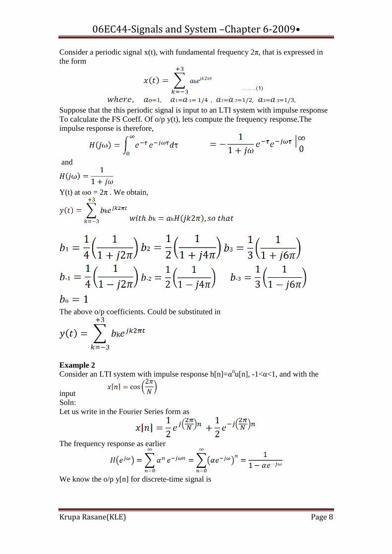
Consider a periodic signal x(t), with fundamental frequency 2π, that is expressed in
the form
Suppose that the this periodic signal is input to an LTI system with impulse response
To calculate the FS Coeff. Of o/p y(t), lets compute the frequency response.The
impulse response is therefore,
and
Y(t) at ωo = 2π . We obtain,
The above o/p coefficients. Could be substituted in
Example 2
Consider an LTI system with impulse response h[n]=αnu[n], -1<α<1, and with the
input
Soln:
Let us write in the Fourier Series form as
The frequency response as earlier
We know the o/p y[n] for discrete-time signal is

06EC44-Signals and System –Chapter 6-2009•
Krupa Rasane(KLE) Page 9
Substituting in the above we get the Fourier series for the output:
If we write
then y[n] reduces to
Finding the Frequency Response
We can begin to take advantage of this way of finding the output for any input once
we have H(ω).
To find the frequency response H(ω) for a system, we can:
1. Put the input x(t) = eiωt
into the system definition
2. Put in the corresponding output y(t) = H(ω) eiωt
3. Solve for the frequency response H(ω). (The terms depending on t will
cancel.)
06EC44-Signals and System –Chapter 6-2009•
Krupa Rasane(KLE) Page 10

06EC44-Signals and System –Chapter 6-2009•
Krupa Rasane(KLE) Page 11
The output of a system in response to an input is .
Find the frequency response and the impulse response of this system.
• Soln:
Summaries Fourier in LTI
• The LTI system scales the complex exponential eiωt
.
• Each system has its own constant H(ω) that describes how it scales
eigenfunctions. It is called the frequency response.
• The frequency response H(ω) does not depend on the input. It is another way
to describe a system, like (A, B, C, D), h, etc.
• If we know H(ω), it is easy to find the output when the input is an
eigenfunction. y(t)=H(ω)x(t) true when x is eigenfunction!
Differential and Difference Equation Descriptions
Frequency Response is the system‟s steady state response to a sinusoid. In contrast to
differential and difference-equation descriptions for a system, the frequency response
description cannot represent initial conditions, it can only describe a system in a
steady state condition. The differential-equation representation for a continuous-time
system is
Rearranging the equation we get

06EC44-Signals and System –Chapter 6-2009•
Krupa Rasane(KLE) Page 12
The frequency of the response is
Hence, the equation implies the frequency response of a system described by a linear
constant-coefficient differential equation is a ratio of polynomials in jω.
The difference equation representation for a discrete-time system is of the form.
Take the DTFT of both sides of this equation, using the time-shift property.
To obtain
• Rewrite this equation as the ratio
• The frequency response is the polynomial in
Differential Equation Descriptions
Ex: Solve the following differential Eqn using FT.
For all t where, .
Soln:we have
FT gives,

06EC44-Signals and System –Chapter 6-2009•
Krupa Rasane(KLE) Page 13
Hence we have
And
i.e
06EC44-Signals and System –Chapter 6-2009•
Krupa Rasane(KLE) Page 14
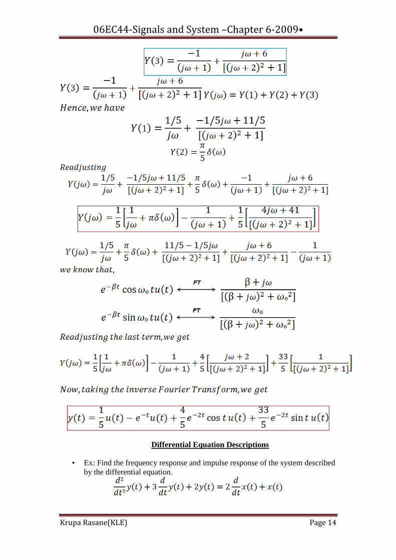
Differential Equation Descriptions
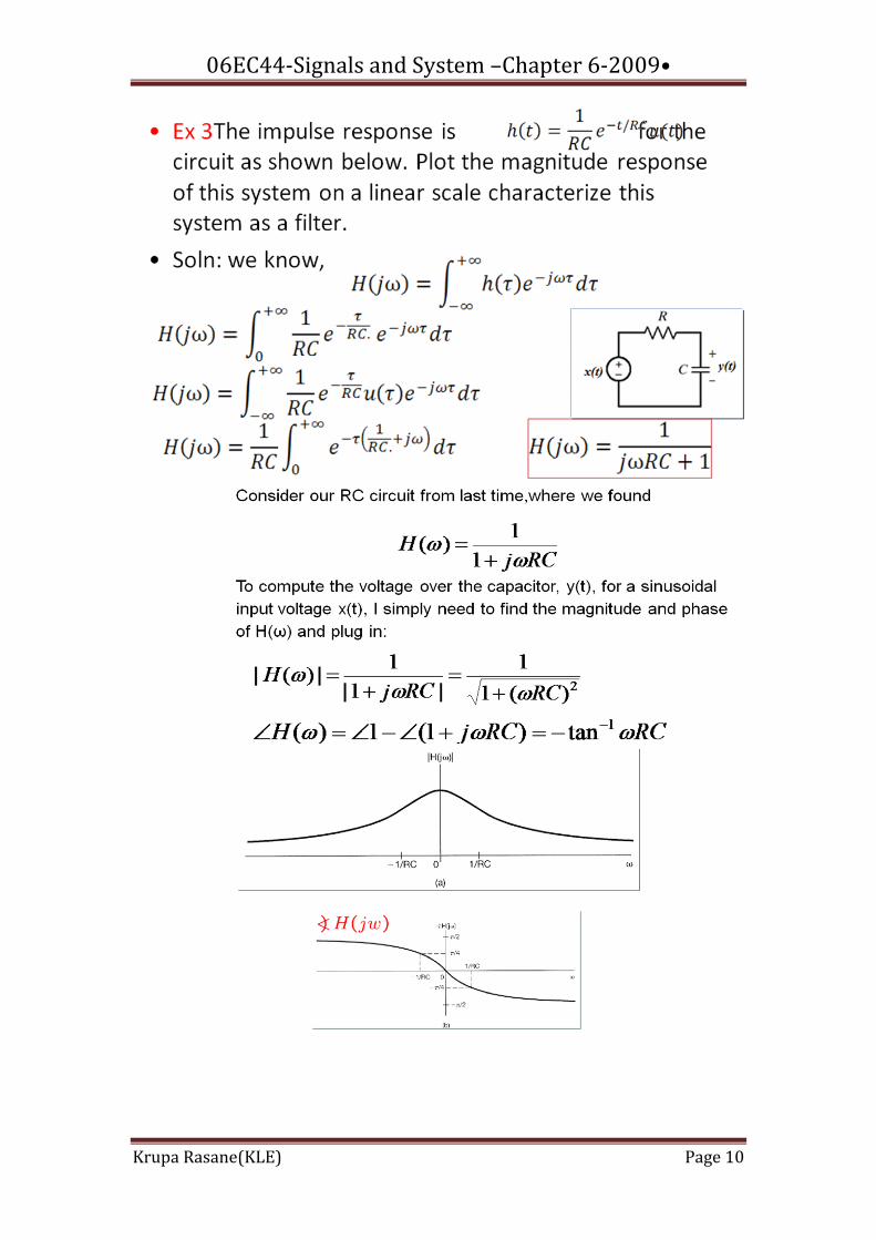
• Ex: Find the frequency response and impulse response of the system described
by the differential equation.
06EC44-Signals and System –Chapter 6-2009•
Krupa Rasane(KLE) Page 15
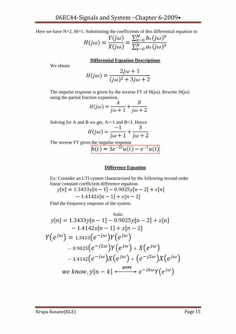
Here we have N=2, M=1. Substituting the coefficients of this differential equation in
Differential Equation Descriptions
We obtain
The impulse response is given by the inverse FT of H(jω). Rewrite H(jω)
using the partial fraction expansion.
Solving for A and B we get, A=-1 and B=3. Hence
The inverse FT gives the impulse response
Difference Equation
Ex: Consider an LTI system characterized by the following second order
linear constant coefficient difference equation.
Find the frequency response of the system.
Soln:

06EC44-Signals and System –Chapter 6-2009•
Krupa Rasane(KLE) Page 16
Ex: If the unit impulse response of an LTI System is h(n)=αnu[n], find the response of
the system to an input defined by where
Soln:

06EC44-Signals and System –Chapter 6-2009•
Krupa Rasane(KLE) Page 17
Sampling In this chapter let us understand the meaning of sampling and which are the different
methods of sampling. There are the two types. Sampling Continuous-time signals and
Sub-sampling. In this again we have Sampling Discrete-time signals.
Sampling Continuous-time signals
Sampling of continuous-time signals is performed to process the signal using digital
processors. The sampling operation generates a discrete-time signal from a
continuous-time signal.DTFT is used to analyze the effects of uniformly sampling a
signal.Let us see, how a DTFT of a sampled signal is related to FT of the continuous-
time signal.
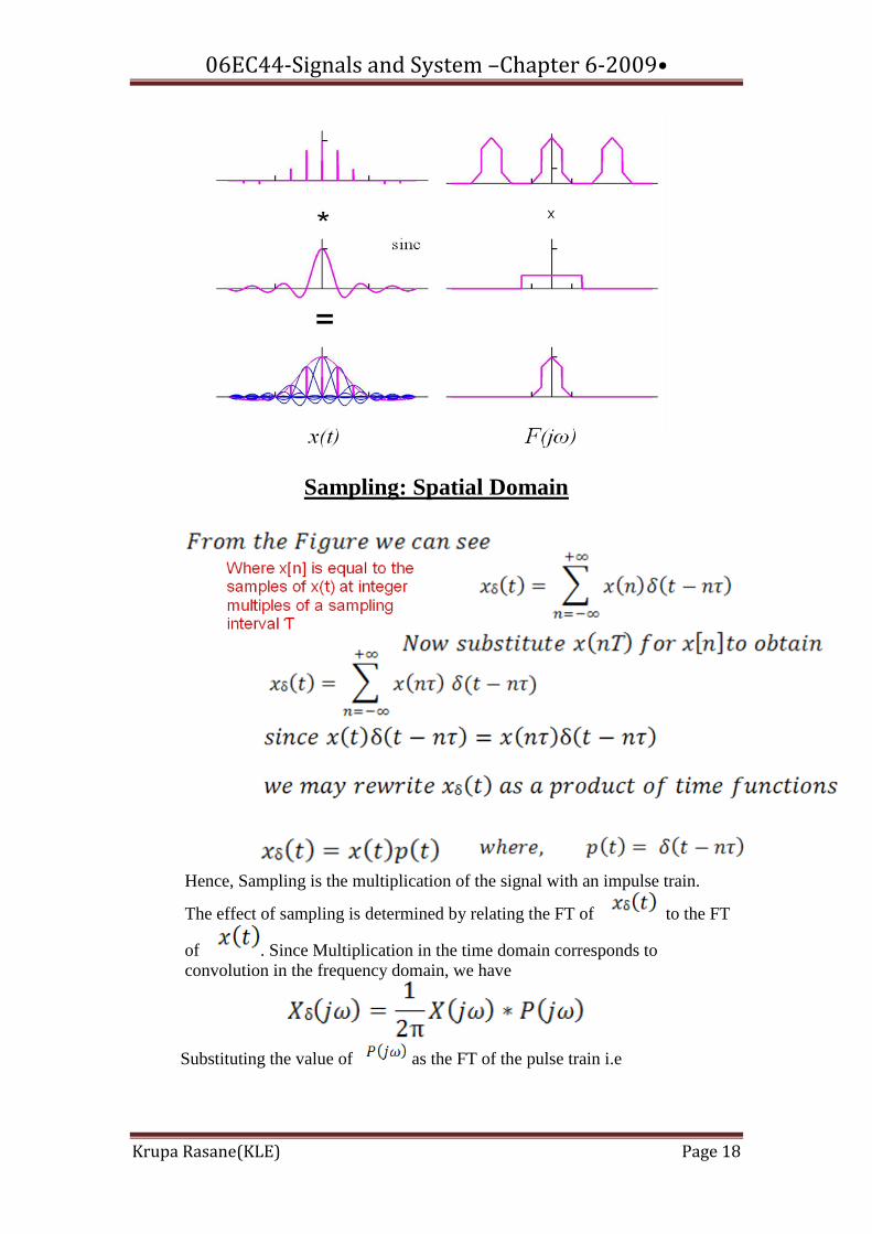
• Sampling: Spatial Domain: A continuous signal x(t) is measured at fixed
instances spaced apart by an interval „Ƭ‟. The data points so obtained form a
discrete signal x[n]=x[nƬ]. Here, ΔƬ is the sampling period and 1/ ΔƬ is the
sampling frequency.Hence, sampling is the multiplication of the signal with an
impulse signal.
• Sampling theory
• Reconstruction theory
06EC44-Signals and System –Chapter 6-2009•
Krupa Rasane(KLE) Page 18
Sampling: Spatial Domain
Hence, Sampling is the multiplication of the signal with an impulse train.
The effect of sampling is determined by relating the FT of to the FT
of . Since Multiplication in the time domain corresponds to
convolution in the frequency domain, we have
Substituting the value of as the FT of the pulse train i.e

06EC44-Signals and System –Chapter 6-2009•
Krupa Rasane(KLE) Page 19
We get,
The FT of the sampled signal is given by an infinite sum of shifted version of
the original signals FT and the offsets are integer multiples of ωs.
Aliasing : an example
Frequency of original signal is 0.5 oscillations per time unit). Sampling
frequency is also 0.5 oscillations per time unit). Original signal cannot be
recovered.
Aliasing Ex:1
Aliasing Ex:2

06EC44-Signals and System –Chapter 6-2009•
Krupa Rasane(KLE) Page 20
Non-Aliasing: Ex 3
Sampling below the Nyquist rate

06EC44-Signals and System –Chapter 6-2009•
Krupa Rasane(KLE) Page 21
Reconstruction below the Nyquist rate
06EC44-Signals and System –Chapter 6-2009•
Krupa Rasane(KLE) Page 22
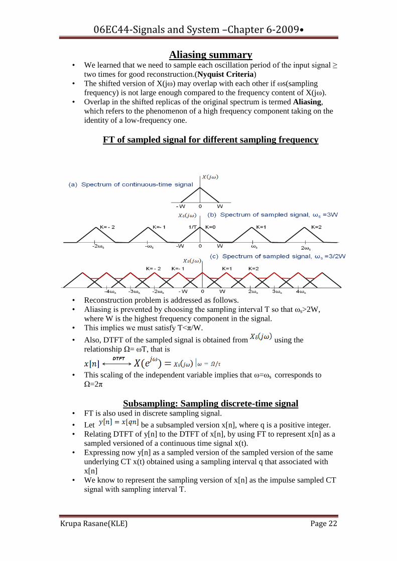
Aliasing summary • We learned that we need to sample each oscillation period of the input signal ≥
two times for good reconstruction.(Nyquist Criteria)
• The shifted version of X(jω) may overlap with each other if ωs(sampling
frequency) is not large enough compared to the frequency content of X(jω).
• Overlap in the shifted replicas of the original spectrum is termed Aliasing,
which refers to the phenomenon of a high frequency component taking on the
identity of a low-frequency one.
FT of sampled signal for different sampling frequency
• Reconstruction problem is addressed as follows.
• Aliasing is prevented by choosing the sampling interval Ƭ so that ωs>2W,
where W is the highest frequency component in the signal.
• This implies we must satisfy Ƭ<π/W.
• Also, DTFT of the sampled signal is obtained from using the
relationship Ω= ωƬ, that is
• This scaling of the independent variable implies that ω=ωs corresponds to
Ω=2π
Subsampling: Sampling discrete-time signal • FT is also used in discrete sampling signal.
• Let be a subsampled version x[n], where q is a positive integer.
• Relating DTFT of y[n] to the DTFT of x[n], by using FT to represent x[n] as a
sampled versioned of a continuous time signal x(t).
• Expressing now y[n] as a sampled version of the sampled version of the same
underlying CT x(t) obtained using a sampling interval q that associated with
x[n]
• We know to represent the sampling version of x[n] as the impulse sampled CT
signal with sampling interval Ƭ.
06EC44-Signals and System –Chapter 6-2009•
Krupa Rasane(KLE) Page 23
• Suppose, x[n] are the samples of a CT signal x(t), obtained at integer multiples
of Ƭ. That is, x[n]=x[nƬ]. Let and applying it to obtain
• Since y[n] is formed using every qth sample of x[n], we may also express y[n]
as a sampled version of x(t).we have
• Hence, active sampling rate for y]n] is Ƭ‟=qƬ. Hence
• Hence substituting Ƭ‟=q Ƭ, and ωs„= ωs/q
• We have expressed both as a function of .
• Expressing as a function of . Let us write k/q as a proper
function, we get

06EC44-Signals and System –Chapter 6-2009•
Krupa Rasane(KLE) Page 24
Summaries Fourier in LTI
• The LTI system scales the complex exponential eiωt
.
• Each system has its own constant H(ω) that describes how it scales
eigenfunctions. It is called the frequency response.
• The frequency response H(ω) does not depend on the input. It is another way
to describe a system, like (A, B, C, D), h, etc.
• If we know H(ω), it is easy to find the output when the input is an
eigenfunction. y(t)=H(ω)x(t) true when x is eigenfunction!
References
• Figures and images used in these lecture notes are adopted from “Signals &
Systems” by Alan V. Oppenheim and Alan S. Willsky, 1997
• Feng-Li Lian, NTU-EE and Mark Fowler Signals and Systems.
• Text and Reference Books have been referred during the notes preparation.
• References • Figures and images used in these lecture notes are adopted from “Signals &
Systems” by Alan V. Oppenheim and Alan S. Willsky, 1997
• Feng-Li Lian, NTU-EE and Mark Fowler Signals and Systems.
• Text and Reference Books have been referred during the notes preparation.


![A Design for Quality Improvement in Remote Higher ...linc.mit.edu/linc2013/proceedings/Session9/Session9Thiruvaazhi.pdf · Source: FICCI Higher Education Summit 2012 Report [4] 1The](https://static.fdocuments.us/doc/165x107/604ea5595540c001ed6547a8/a-design-for-quality-improvement-in-remote-higher-lincmitedulinc2013proceedingssession9.jpg)