06709789

IEEE TRANSACTIONS ON POWER SYSTEMS, VOL. 29, NO. 4, JULY 2014 1503

Calculation of Power Transfer Limit ConsideringElectro-Thermal Coupling of Overhead

Transmission LineXiaoming Dong, Member, IEEE, Chengfu Wang, Jun Liang, Xueshan Han, Feng Zhang, Hua Sun,

Mengxia Wang, and Jingguo Ren

Abstract—In this paper, new formulations of the power flow andcontinuation power flow that allow for electro-thermal couplingin transmission lines have been proposed. The new formulationscapture the overhead lines’ electro-thermal coupling effects bytreating their series resistances as temperature dependent vari-ables. They generate results that can differ from the results ofconventional formulations markedly, particularly for problemscentring on line impedances. The paper demonstrates this byapplying the new formulations to the power transfer limit cal-culation. Generally, power transfer limits are defined either byencountering a line’s thermal limit or detecting the onset of voltagecollapse in the system. Studies based on 2-bus and 14-bus testsystems are used to demonstrate the efficacy of the new formula-tions for both situations. For these studies, specific point-to-pointpower transfer limits are calculated with and without the lines’electro-thermal coupling effects and the results are compared.

Index Terms—Continuation method, electro-thermal coupling,power flow, saddle-node bifurcation, thermal limit.

I. INTRODUCTION

A central problem in electricity markets is establishing themaximum power that can be safely transferred between a

generating plant and a load center, known as the power transferlimit (PTL). In PTL formulation, the PTL is reached when thetemperature, or alternatively the current, of a transmission linereaches its allowable level, called thermal limit (TL) [1]–[8]. Al-ternatively, with the rampant increase in voltage stability (VS)problems, the PTL could be defined by encountering a systemvoltage collapse point, also known as the saddle-node bifurca-tion (SNB) point [9]–[13]. In either case, values of the PTLs areheavily influenced by the characteristics of the lines forming thepower network.

Manuscript received August 12, 2012; revised December 19, 2012, April 24,2013, August 18, 2013, and October 08, 2013; accepted December 17, 2013.Date of publication January 10, 2014; date of current version June 16, 2014.This work was supported by the National Natural Science Foundation of China(No. 51307101, 51177091, and 51077087), the Science-Technology Founda-tion for Middle-aged and Young Scientist of Shandong Province, China (No.BS2013NJ011). Paper no. TPWRS-00833-2012.X. Dong and C. Wang are with the Department of Electrical Engineering, Ts-

inghua University, Beijing 100084, China (e-mail: [email protected]).J. Liang, X. Han, F. Zhang, M. Wang, and J. Ren are with the School of

Electrical Engineering, Shandong University, Jinan 250061, China (e-mail:[email protected]).H. Sun is with the Department of Electrical Automation, Shandong Labour

Vocational and Technology College, Jinan 250022, China.Digital Object Identifier 10.1109/TPWRS.2013.2296553

An effective method for PTL evaluation is the power flow(PF) simulation. It involves gradual increases in power demandsat receiving buses, while maintain the power balance by ad-justing outputs of sending generators, until a device operatinglimit is encountered. In some cases, before encountering an op-erating limit, the system state approaches an SNB point, ren-dering the PF Jacobian matrix ill-conditioned and the PF iter-ations non-convergent. An approach that allows running PFsvery close to an SNB point is the continuation power flow (CPF)[14]–[19], which is based on the principles of the ContinuationMethod (CM).In the conventional PF and CPF formulations, line series re-

sistances are treated as fixed, ignoring their variations with linecurrents. This approximation introduces an error in the resultingPTLs that, for certain class of power grids, could be significant.Therefore, an objective of this paper is to indicate how largesuch errors can become and which power grids tend to mag-nify them. Note that, as the primary focus of this study is onthe relationships among line current, temperature, and series re-sistance, impacts of atmospheric/meteorological conditions onthese quantities are ignored here.The rest of the paper is organized as follows: Section II

reveals that, even for a primitive power system, line resis-tance changes alter the SNB point. In Section III, steady-stateelectro-thermal coupling (ETC) equations [2]–[8] are derivedfrom dynamic heat balance relations of overhead transmissionlines (OTL). Using the analyses of Sections II and III, inSection IV the ETC power flow (ETC-PF) model is proposed.Then, in Section V flow diagrams detailing the steps com-prising the ETC-PF and ETC-CPF procedures are presented.Section VI deploys two case studies to show the degree atwhich PTL values can be influenced by the new formulations.In Section VII, the main results are summarized and key con-clusions are recapped.

II. SNB ANALYSIS WITH CHANGING RESISTANCE

In Fig. 1, is the voltage source magnitude;is the branch series impedance; and

is the load impedance. As shown in (1), the critical value ofthe power demand , defining the SNB, is solelydetermined by , and .

(1)

0885-8950 © 2014 IEEE. Personal use is permitted, but republication/redistribution requires IEEE permission.See http://www.ieee.org/publications_standards/publications/rights/index.html for more information.

1504 IEEE TRANSACTIONS ON POWER SYSTEMS, VOL. 29, NO. 4, JULY 2014

Fig. 1. Schematic diagram of a simple radial power system.

Fig. 2. Relationship between and .

Fig. 3. Relationship between and .

with

(2)

The sensitivity of to changes in is given by

(3)

With the assumption that per unit (p.u.) andp.u., the relationship between and is shown in

Fig. 2. When the load power factor is fixed, an increase incauses to decline.As shown in Fig. 3, the sensitivity of to increases

with higher power factors. To reduce power loss and providevoltage support, shunt capacitors are deployed extensively atbuses serving large loads. Hence, load buses are usually oper-ated at high power factors, causing the increases in to havehigher impacts on and .

III. STEADY-STATE ETC

It is assumed that all overhead conductors (OCs) of a three-phase OTL operate nearly under the same atmospheric/mete-orological conditions and have the same physical properties,counting the thermal ones. The dynamic heat balance equationsfor each OC are the same and are expressed as follows:

(4)

(5)

(6)

(7)

In the above relations, is the length of the OC; is its unitweight; , and represent the manufacturer-supplied ref-erence values for resistance, temperature, and temperature co-efficient, respectively; , , and are the OC actual seriesresistance, temperature and current, respectively; is its am-bient temperature; is the heat capacity of its material, whileand are its convective and radiation heat transfer coef-

ficients, respectively. For each per unit length of the OC, isits absorbed heat rate; is its convective heat rate and is itsradiation rate.For systems with slow varying demands, one can assume

. That is, the OTLs heat balance dynamics can beignored, as they are generally slow, long-term, processes. Thatremoves time, , from the equations, allowing (4) to be restatedas

(8)

Since and of the th OTL are per-unit quantities, it fol-lows that

(9)with

(10)

(11)

(12)

where index “ ” refers to the th OTL and , , and areline’s per-unit values for , , and , respectively; is thesystem base MVA; is the phase base impedance of the thOTL; is the base voltage of the th OTL; and representsboth the line base current and the phase base current of the thOTL under the assumption that the three-phase OTL is star con-nected. Then, (9) is expressed in its compact form by

(13)

The assumption that all OTL conductors are constructed fromthe same material implies their thermal characteristics are thesame and a single set of parameters can be used to define them.

DONG et al.: CALCULATION OF POWER TRANSFER LIMIT CONSIDERING ELECTRO-THERMAL COUPLING OF OVERHEAD TRANSMISSION LINE 1505

TABLE ILINE THERMAL BEHAVIOR COEFFICIENT

TABLE IILINE PARAMETERS

Fig. 4. Diagram of the relationship among , , and .

Table I contains the parameters used in Section VI to analyzecase studies. The line parameters are set as shown in Table II.As shown in Fig. 4, and increase approximately linearly

with increases in .

IV. ETC POWER FLOW

With all of line parameters expressed as per-unit values, theconventional PF equations are expressed as

(14)

where is the total number of network buses; and are theactive power and reactive power injected into network at bus ,respectively; is the voltage magnitude at bus ;is the phase angle between complex bus voltages and

; and are the self-conductance and self-suscep-tance at bus , respectively; and and are the mutualconductance and mutual susceptance, respectively, between busand . In its compact form, (14) is expressed as follows:

(15)

where

(16)

(17)

When conductance and susceptance are expressed in terms ofresistance and reactance

(18)

(19)

where and are the resistance and reactance, respec-tively, between bus and bus . Under the assumption that theth OTL is star connected, the phase current is equal to the linecurrent and is expressed as follows:

(20)

where indicates that bus and bus are the terminalbuses of the th OTL and is expressed in form of . Thefollowing equations are derived from (20):

(21)

Equation (18) is abbreviated as follows:

(22)

Equation (23) is derived from (13) and (22):

(23)

The equations in (24), which treat OTL series resistances asPF variables, represent the ETC-PF model:

...

...

(24)

where is the number of OTLs. Vector represents the seriesresistances:

(25)

The ETC-PF solution vector, , is comprised of the unknownvectors , and ; that is

(26)


To solve the nonlinear, algebraic, equations in (24), the iter-ative scheme of (27) is deployed:

(27)

where and represent the steps of the iterations.The following inequality is used as the convergence standard

of the Newton iteration process:

(28)

where is a small positive number that is given in advance.In (27), represents the extended Jacobian matrix, which is

expressed as follows:

(29)

where is the conventional Jacobian matrix. The elements ofthe matrix are given by the following relations:

(30)

with

(31)

The elements of the matrix are given by the fol-lowing relations:

(32)

with

(33)

The elements of the matrix are given by the followingrelations:

(34)

with

(35)The elements of the matrix are given by the following

relations:

(36)

with

(37)

V. ETC-PF AND ETC-CPF PROCEDURES

To avoid ill-conditioning problems at and near the SNB, theETC-CPF model is derived (see the Appendix). Then, a com-puter program consisting of the ETC-PF and ETC-CPF modelsis designed, and its flow diagram is given in Fig. 5. At the begin-ning of ETC-PF, an initial point must be given for the iterationprocess. Variables representing line series resistances are initial-ized to their rated values. Voltagemagnitudes and voltage anglesare initialized for a “flat start”. Through iterative calculation, thenumerical solutions of the ETC-PF equations and the base pointof ETC-CPF are obtained. This base point is generallyin accordance with typical system operating conditions such aswinter peak or summer peak. Once the base point is given, withalternating predictor and corrector steps, the ETC-CPF modeltraces the solutions of the parametric load flow equation aschanges ( , ). It simulates the process where theelectric power demand and generation are increased graduallyuntil the SNB is reached .

VI. CASE STUDIES

In this section the new formulations are applied to two casestudies to show how ETC can influence power grid’s transferlimits. For each test system a specific point-to-point powertransfer limit is calculated with and without the ETC effect andthe results are compared.Case 1 is a simple two-bus power system, comprised of a gen-

erator and a load, connected by an OTL. The simplicity of thiscase allows one to explore the impacts of various system pa-rameters on PTL in the presence of ETC, including load powerfactor and line length.Case 2 is the IEEE 14-bus system, which consists of 5 gener-

ation buses and 11 load points, interconnected by 17 lines andtransformers. In this system, power generation and distributionare performed at 34.5 kV, while power transmission is accom-plished via 138-kV lines. As shown in Fig. 10, here the powertransfer limit of interest is point-to-point, between the generatorbus 1 and the load at bus 10.Case 1: Table I specifies the thermal characteristics of the

line in the test system of Fig. 6. The values for other parametersdescribing the system are provided in Tables III and IV.

, which is set to , denotes the value of at the beginningof ETC-PF simulation; and are respectively the load’s ac-tive and reactive power components.


Fig. 5. Flow diagram of ETC-CPF.

Fig. 6. Simple test power system.

TABLE IIIOVERHEAD TRANSMISSION LINE PARAMETERS

TABLE IVCPF CALCULATING PARAMETERS

In Fig. 7, PV (1) is obtained using the conventional CPFmodel; PV (2) and the resistance curves are obtained using theETC-CPF model. The differences between PV (1) and PV (2)

Fig. 7. PV curves and the line resistance curve.

TABLE VRESULTS CALCULATED BY THE TWO METHODS

are the result of ignoring the ETC. Some specific data are givenin Table V for comparison.In Table V, is the critical active power at the SNB

point; is the critical series resistance at the SNB point;is the initial value; and denotes the solution of the

ETC-PF model as well as the base point of ETC-CPF. Asshown in Table V, when using conventional CPF, ,and are all equal to due to ignore the ETC. However,when ETC is taken into account, there exists a 6.25% marginof error between and , which are 0.0880 and 0.0935,respectively. At the critical point in ETC-CPF, reaches0.1142, with a 24% margin of error compared to . In Fig. 7,the critical powers and are calculated by the con-ventional method and the ETC-CPF model, respectively. Toquantitatively express the error between the two methods, thefollowing parameter is defined:

(38)

In Fig. 7, is approximately 6.9%; however, its value varieswith various trajectories (representing the scaling up of andQ).In Fig. 8, the OB trajectory represents the growth path of

the load power; point O denotes the base point; point A andpoint B denote the SNB points obtained by the two methods,respectively; and point C represents the value of . Points A,B, and C are all related to the trajectory OB. As shown in Fig. 8,is larger with greater proportions of active power.Because the line series impedance is highly correlated with

the line length , the results of ETC-CPF will vary due tochanges in . Critical line temperature , correspondingto different , can be produced by ETC-CPF. , introducedas TL, is set to 70 . Then, as shown in Fig. 9, the relationship


Fig. 8. SNB boundary comparison and error analysis.

Fig. 9. Relationship among , SNB, and TL.

among SNB, TL, and is revealed by comparing and.When is longer than 119 km, is lower than .

It implies that the SNB is the major limitation for long-distancepower transmission; on the other hand, more attention must bepaid to TL for short-distance power transmission.Case 2: In this case, an IEEE 14-bus test system (see Fig. 10)

is analyzed using both the conventional method and the newmethod. The is set to 100 MW. Some line parametersare modified and supplemented as shown in Table VI. isthe line charging capacitance. In traditional system studies, lineoverloads are decided by comparing line currents against theirmaximum allowable currents, . A line’s , also knownas its TL, is obtained using (9) with ; that is shownin (39) at the bottom of the page.The values given in Table VI are obtained using (39)

with . The lines thermal coefficients used incalculations are those given in Table I.It is assumed that power consumption at bus 10 will be in-

creased to meet the energy demands of new factories, plannedto be constructed in that vicinity. To satisfy the future demandsat bus 10, one option is to transfer power from bus 1 to bus 10.

Fig. 10. IEEE 14-bus test system.

TABLE VILINE PARAMETERS OF THE IEEE 14-BUS TEST SYSTEM

Establishing the feasibility of this option, that is whether bus 1can in fact supply sufficient power to bus 10, requires a PTLanalysis. This analysis entails increasing the active power at

(39)


Fig. 11. Analysis with conventional CPF.

bus 10 in steps and supplying from bus 1 the resulting systempower imbalance. Below the results of applying to this problemthe conventional CPF, as well as ETC-CPF, are discussed.The trend lines in Fig. 11 are obtained using conventional

CPF. They show increases in the OTL currents, as the activepower demand at bus 10 is increased. Parameter , defined by

(40)

has been introduced here to indicate the available loading ca-pacity of each line at each demand level. When for a line ,that line is fully loaded and any further increase in the demandat bus 10 leads to its overload.As observed in Fig. 11, using the conventional CPF steps,

the first over-current OTL is bus6–bus11,followed by bus9–bus10, bus7–bus9, bus10–bus11, andbus6–bus13. Therefore, based on CPF analysis, the maximumactive power that can be served at bus 10 (that is, ) is 0.627p.u., while is 2.340 p.u..The trends of line temperatures obtained by ETC-CPF

are shown in Fig. 12. The first over-temperatureOTL is bus6–bus11, followed by bus7–bus9, bus9–bus10 and soon. and are 0.544 p.u. and 1.506 p.u., respectively,which are significantly different from the results of the conven-tional method. The differences between these values and theirCPF counterparts are simply due to OTL resistances changingwith their line temperatures. The results of the ETC-CPF areexpected to be more accurate because it is based on a more pre-cise representation of the OTL operation. The PTL values pro-duced by CPF are consistently larger than those generated byETC-CPF. As such, using CPF without a large safety margincould lead to transmission system expansion plans that may fallshort of their stipulated power transfer goals.Discussion: The IEEE 14-bus system, which is used in con-

structing Case 2, is a special low voltage network. As shown inTable VI, the majority of the lines in this system havevalues that are above 1/4 and a good many of the lines have

values that are approximately 1/2. In this case, the in-fluence of electro-thermal coupling is considerable. However,

Fig. 12. Analysis with ETC-CPF.

for high voltage networks, the lines’ values are typicallymuch smaller. Therefore, it is reasonable to expect that the influ-ence of electro-thermal coupling on high voltage power grids tobe much smaller than those indicated by Case 2. In other words,the differences in the values of and , produced byCPF and ETC-CPF, would be markedly smaller.

VII. CONCLUSIONS

Traditional calculation of power transfer limits neglects theelectro-thermal coupling in overhead transmission lines. Thisresults in overestimating the power transfer limits, the extentof which can be significant for certain systems. In this paper, anew power flow formulation that takes into account the electro-thermal couplings of overhead transmission lines is introduced.Then, using the Continuation Method framework, it has beenused to calculate the power transfer limits for two study cases.The results obtained for Case 2, which uses the IEEE 14-bus

test system, indicate 13.45% error in the value of a powertransfer limit, when it is calculated using the conventionalmethod and defined by the lines’ thermal limits. This errorincreases to 34% when the power transfer is limited by theonset of voltage collapse in the power grid.For low voltage networks, the errors in the values of power

transfer limits can be substantial. These errors are not typical ofhigh voltage networks, where ratios of line resistances to theirreactances are generally very small.Compared with traditional models of transmission lines, the

proposed method uses a more detailed representation for theoverhead transmission lines. Therefore, with accurate model pa-rameters, it is capable of consistently producing more precise,and therefore more reliable, values for power transfer limits.

APPENDIXETC-CPF MODEL

The ETC-CPF model consists of four parts:


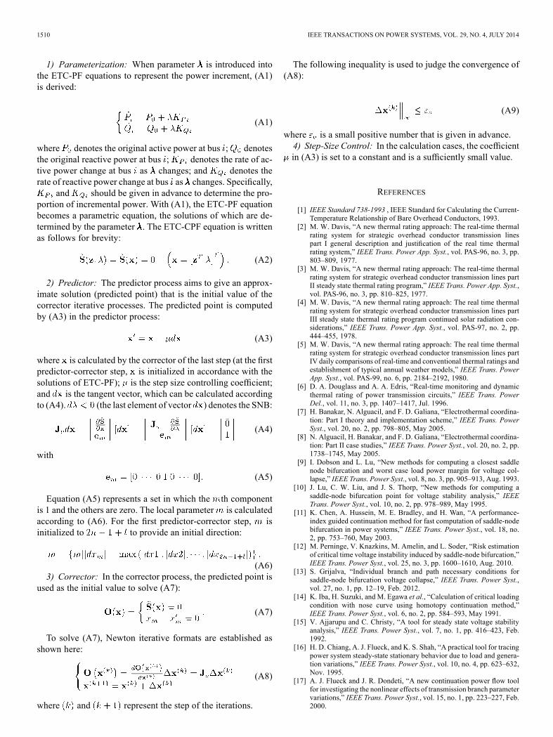
1) Parameterization: When parameter is introduced intothe ETC-PF equations to represent the power increment, (A1)is derived:

(A1)

where denotes the original active power at bus ; denotesthe original reactive power at bus ; denotes the rate of ac-tive power change at bus as changes; and denotes therate of reactive power change at bus as changes. Specifically,

and should be given in advance to determine the pro-portion of incremental power. With (A1), the ETC-PF equationbecomes a parametric equation, the solutions of which are de-termined by the parameter . The ETC-CPF equation is writtenas follows for brevity:

(A2)

2) Predictor: The predictor process aims to give an approx-imate solution (predicted point) that is the initial value of thecorrector iterative processes. The predicted point is computedby (A3) in the predictor process:

(A3)

where is calculated by the corrector of the last step (at the firstpredictor-corrector step, is initialized in accordance with thesolutions of ETC-PF); is the step size controlling coefficient;and is the tangent vector, which can be calculated accordingto (A4). (the last element of vector ) denotes the SNB:

(A4)

with

(A5)

Equation (A5) represents a set in which the th componentis 1 and the others are zero. The local parameter is calculatedaccording to (A6). For the first predictor-corrector step, isinitialized to to provide an initial direction:

(A6)3) Corrector: In the corrector process, the predicted point is

used as the initial value to solve (A7):

(A7)

To solve (A7), Newton iterative formats are established asshown here:

(A8)

where and represent the step of the iterations.

The following inequality is used to judge the convergence of(A8):

(A9)

where is a small positive number that is given in advance.4) Step-Size Control: In the calculation cases, the coefficientin (A3) is set to a constant and is a sufficiently small value.

REFERENCES

[1] IEEE Standard 738-1993 , IEEE Standard for Calculating the Current-Temperature Relationship of Bare Overhead Conductors, 1993.

[2] M. W. Davis, “A new thermal rating approach: The real-time thermalrating system for strategic overhead conductor transmission linespart I general description and justification of the real time thermalrating system,” IEEE Trans. Power App. Syst., vol. PAS-96, no. 3, pp.803–809, 1977.

[3] M. W. Davis, “A new thermal rating approach: The real-time thermalrating system for strategic overhead conductor transmission lines partII steady state thermal rating program,” IEEE Trans. Power App. Syst.,vol. PAS-96, no. 3, pp. 810–825, 1977.

[4] M. W. Davis, “A new thermal rating approach: The real time thermalrating system for strategic overhead conductor transmission lines partIII steady state thermal rating program continued solar radiation con-siderations,” IEEE Trans. Power App. Syst., vol. PAS-97, no. 2, pp.444–455, 1978.

[5] M. W. Davis, “A new thermal rating approach: The real time thermalrating system for strategic overhead conductor transmission lines partIV daily comparisons of real-time and conventional thermal ratings andestablishment of typical annual weather models,” IEEE Trans. PowerApp. Syst., vol. PAS-99, no. 6, pp. 2184–2192, 1980.

[6] D. A. Douglass and A. A. Edris, “Real-time monitoring and dynamicthermal rating of power transmission circuits,” IEEE Trans. PowerDel., vol. 11, no. 3, pp. 1407–1417, Jul. 1996.

[7] H. Banakar, N. Alguacil, and F. D. Galiana, “Electrothermal coordina-tion: Part I theory and implementation scheme,” IEEE Trans. PowerSyst., vol. 20, no. 2, pp. 798–805, May 2005.

[8] N. Alguacil, H. Banakar, and F. D. Galiana, “Electrothermal coordina-tion: Part II case studies,” IEEE Trans. Power Syst., vol. 20, no. 2, pp.1738–1745, May 2005.

[9] I. Dobson and L. Lu, “New methods for computing a closest saddlenode bifurcation and worst case load power margin for voltage col-lapse,” IEEE Trans. Power Syst., vol. 8, no. 3, pp. 905–913, Aug. 1993.

[10] J. Lu, C. W. Liu, and J. S. Thorp, “New methods for computing asaddle-node bifurcation point for voltage stability analysis,” IEEETrans. Power Syst., vol. 10, no. 2, pp. 978–989, May 1995.

[11] K. Chen, A. Hussein, M. E. Bradley, and H. Wan, “A performance-index guided continuation method for fast computation of saddle-nodebifurcation in power systems,” IEEE Trans. Power Syst., vol. 18, no.2, pp. 753–760, May 2003.

[12] M. Perninge, V. Knazkins, M. Amelin, and L. Soder, “Risk estimationof critical time voltage instability induced by saddle-node bifurcation,”IEEE Trans. Power Syst., vol. 25, no. 3, pp. 1600–1610, Aug. 2010.

[13] S. Grijalva, “Individual branch and path necessary conditions forsaddle-node bifurcation voltage collapse,” IEEE Trans. Power Syst.,vol. 27, no. 1, pp. 12–19, Feb. 2012.

[14] K. Iba, H. Suzuki, and M. Egawa et al., “Calculation of critical loadingcondition with nose curve using homotopy continuation method,”IEEE Trans. Power Syst., vol. 6, no. 2, pp. 584–593, May 1991.

[15] V. Ajjarupu and C. Christy, “A tool for steady state voltage stabilityanalysis,” IEEE Trans. Power Syst., vol. 7, no. 1, pp. 416–423, Feb.1992.

[16] H. D. Chiang, A. J. Flueck, and K. S. Shah, “A practical tool for tracingpower system steady-state stationary behavior due to load and genera-tion variations,” IEEE Trans. Power Syst., vol. 10, no. 4, pp. 623–632,Nov. 1995.

[17] A. J. Flueck and J. R. Dondeti, “A new continuation power flow toolfor investigating the nonlinear effects of transmission branch parametervariations,” IEEE Trans. Power Syst., vol. 15, no. 1, pp. 223–227, Feb.2000.


[18] D. A. Alves, L. C. P. Da Silva, and C. A. Castro et al., “Continuationfast decoupled power flow with secant predictor,” IEEE Trans. PowerSyst., vol. 18, no. 3, pp. 1078–1085, Aug. 2003.

[19] S. H. Li and H. D. Chiang, “Continuation power flow with nonlinearpower injection variations,” IEEE Trans. Power Syst., vol. 23, no. 4,pp. 1637–1643, Nov. 2008.

Xiaoming Dong (M’10) received the Ph.D. degreefrom the School of Electrical Engineering at Shan-dong University, Jinan, China, in 2013.He is currently a Research Associate at Tsinghua

University, Beijing, China. His research interests in-clude power system stability, power system control,and power system operation.

Chengfu Wang received the Ph.D. degree from theSchool of Electrical Engineering at Shandong Uni-versity, Jinan, China, in 2012.He is currently a Research Associate at Tsinghua

University, Beijing, China. His research interests in-clude and power system operation and renewable op-eration and control.

Jun Liang received the Ph.D. degree from theSchool of Electrical Engineering at ShandongUniversity, Jinan, China.He is currently a Professor at Shandong Univer-

sity. His research interests include power system au-tomation, power system operation, and power systemcontrol.

Xueshan Han received the Ph.D. degree from theSchool of Electrical Engineering and Automationat Harbin Institute of Technology, Harbin, China, in1994.He is currently a Professor at Shandong Univer-

sity, Jinan, China. His research interests includepower system generation, power system operation,power system economics and optimization, andelectric power economics.

Feng Zhang is a Lecturer at Shandong University, Jinan, China. His major ispower system operation.

Hua Sun is a Lecturer at Shandong Labour Vocational and Technology College.His major is power system operation.

Mengxia Wang is a Lecturer at Shandong University, Jinan, China. His majoris electrical-thermal coupling approach.

Jingguo Ren is a Doctoral Student at Shandong University, Jinan, China. Hisresearch interests include voltage source converter based dc transmission andmulti-terminal dc transmission.

06709789

Documents

Transcript of 06709789