052600 VU Signal and Image Processing Torsten Möller...
48
052600 VU Signal and Image Processing Torsten Möller + Hrvoje Bogunović + Raphael Sahann [email protected] [email protected] [email protected] vda.cs.univie.ac.at/Teaching/SIP/17s/
Transcript of 052600 VU Signal and Image Processing Torsten Möller...

052600 VUSignal and Image Processing
Torsten Möller + Hrvoje Bogunović + Raphael Sahann
vda.cs.univie.ac.at/Teaching/SIP/17s/
2
3
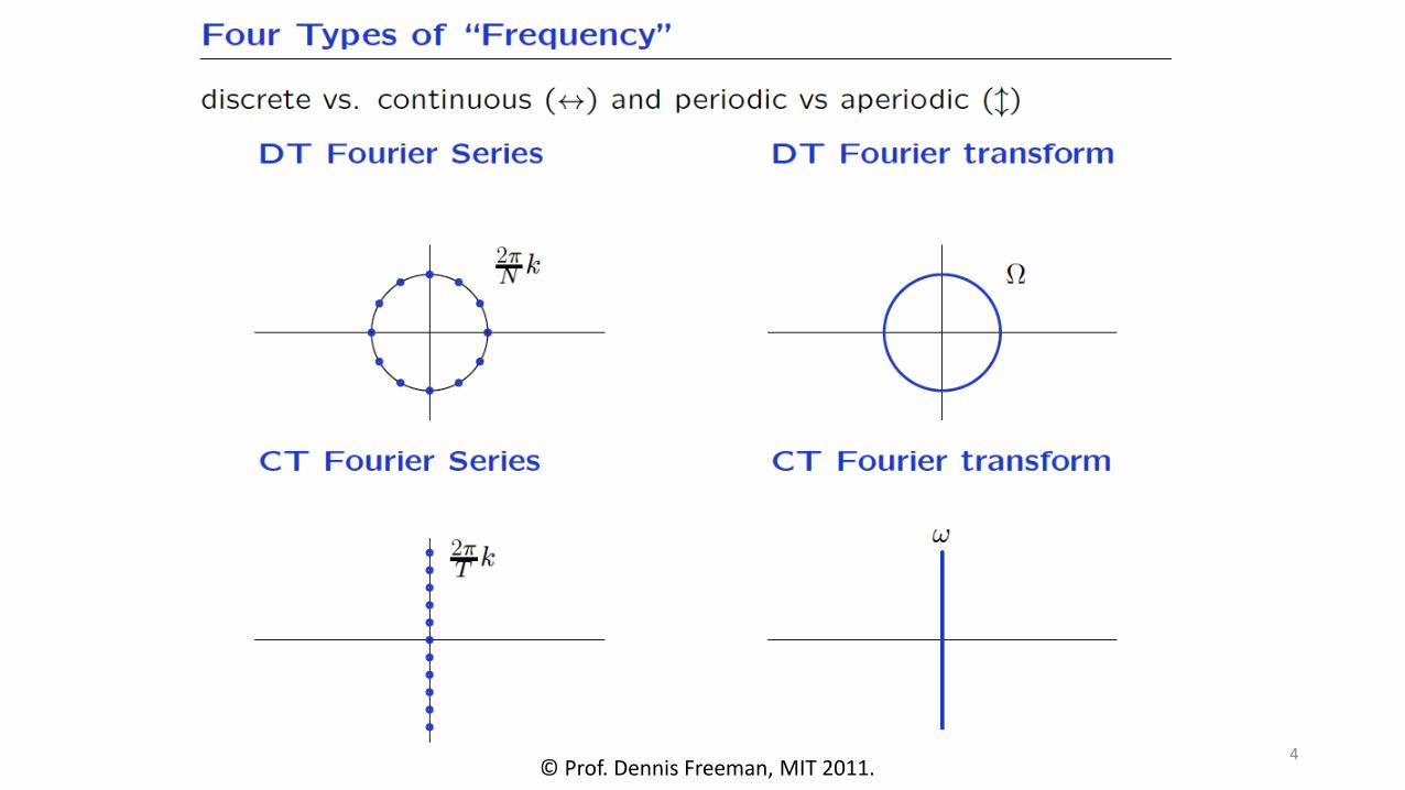
4© Prof. Dennis Freeman, MIT 2011.

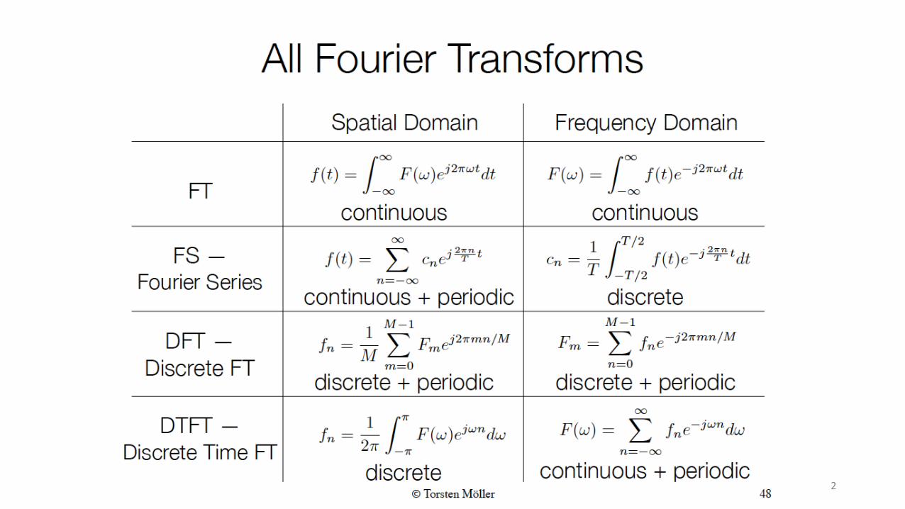
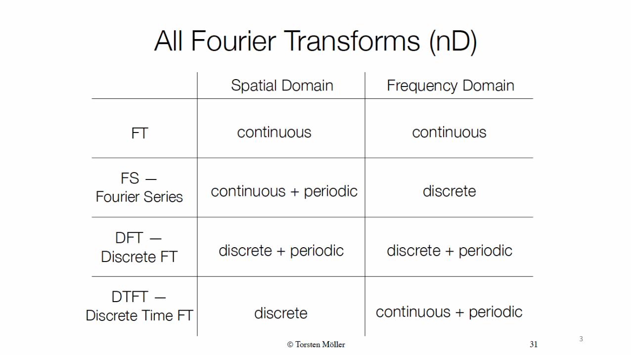
All Fourier Transforms
5© Prof. Branko Jeren, FER, 2010
ContinuousAperiodic
DiscreteAperiodic
ContinuousPeriodic
DiscretePeriodic
CTFT
DTFT
CTFS
DTFS
SIGNAL

DFT - Example
6
N=10
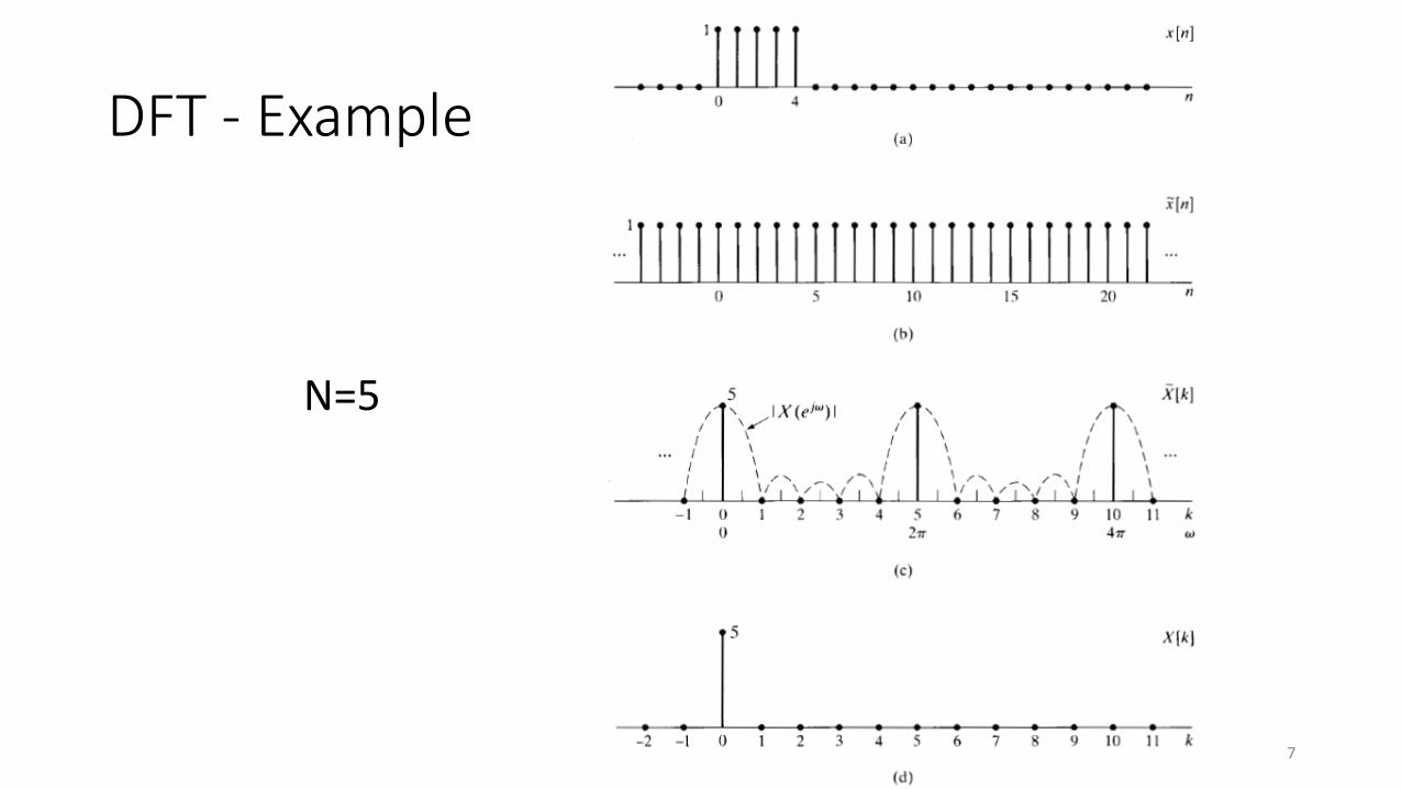
DFT - Example
7
N=5

2D DFT
• DFT of image with M rows and N columns
• IDFT:
8
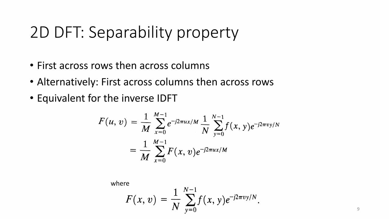
2D DFT: Separability property
• First across rows then across columns
• Alternatively: First across columns then across rows
• Equivalent for the inverse IDFT
9
where
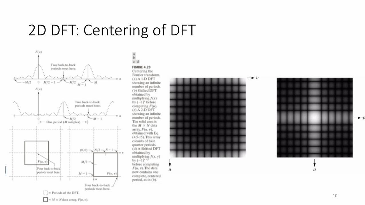
2D DFT: Centering of DFT
10

DFT – propertiesTime-shifting• Inherent periodicity as the
byproduct of DFT
11

DFT – properties: Circular convolution
• Circular convolution: IDFT(DFT(x)*DFT(h))
12

DFT – properties: Circular convolution
• Linear convolution with aliasing
13
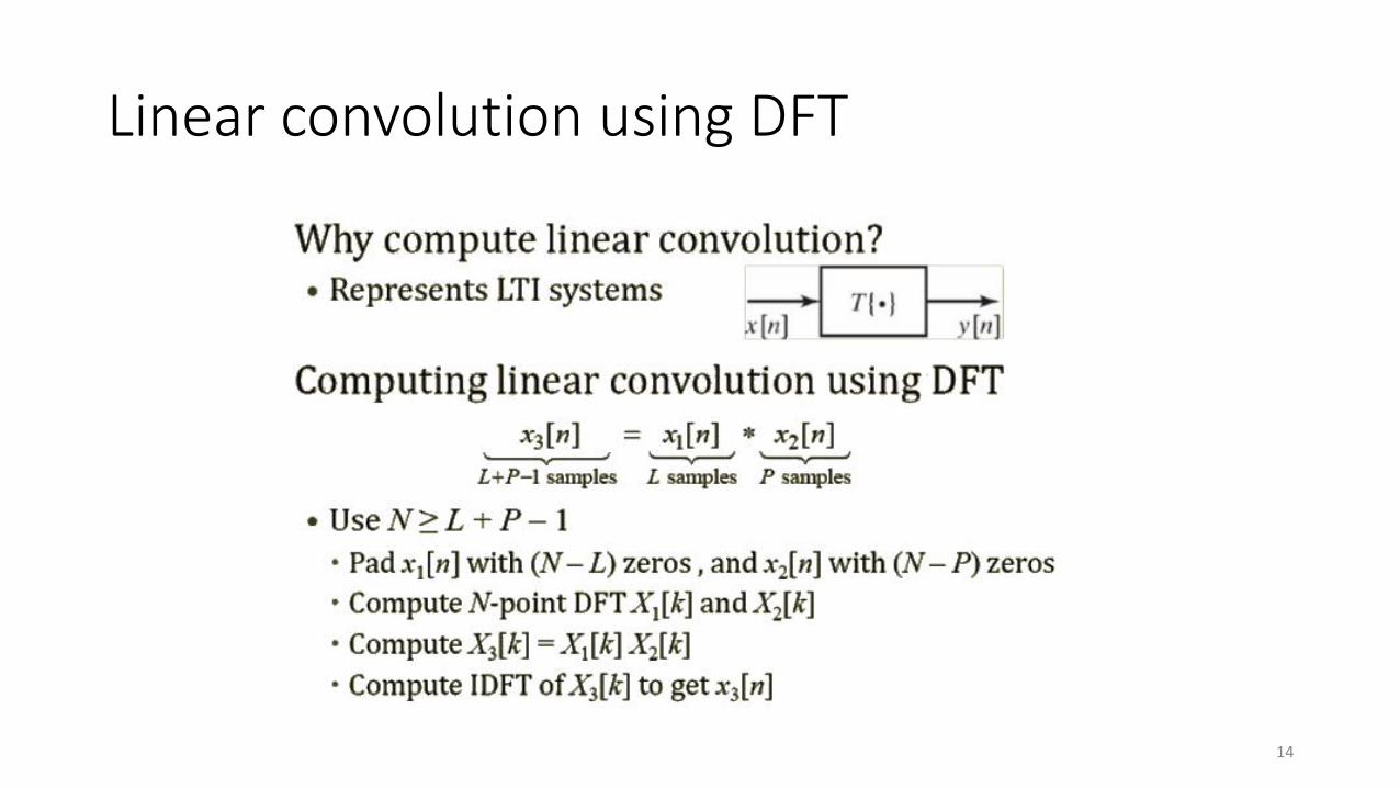
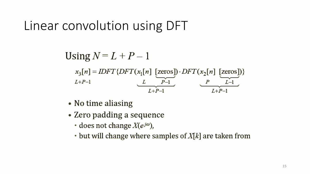
Linear convolution using DFT
14
Linear convolution using DFT
15

Linear convolution using DFT
• Need for zero-padding
• Length N of at least L+P-1
16

Linear convolution using DFT
• Need for zero-padding
• Length N of at least L+P-1
17

18© Prof. Dennis Freeman, MIT 2011.

DFT and FFT: Introduction
• Allows to numerically compute the spectrum of a signal
• Efficient implementation of convolution
• You can also identify impulse response of unknown black-box LTI system• h(t) = IDFT( DFT[y(t)] / DFT[x(t)] )
• Signal coding. With the usage of e.g. DCT (a variant of DFT with real numbers only)• JPEG
• In 1994, Gilbert Strang described the FFT as "the most important numerical algorithm of our lifetime" and it was included in Top 10 Algorithms of 20th Century by the IEEE journal Computing in Science & Engineering.
19

DFT and FFT: Introduction
20© Prof. I. Selesnick
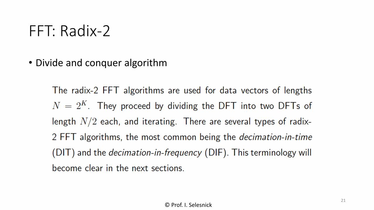
FFT: Radix-2
• Divide and conquer algorithm
21© Prof. I. Selesnick
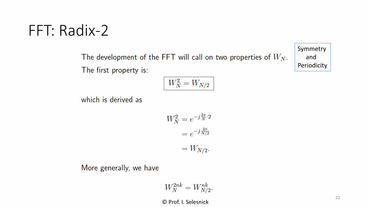
FFT: Radix-2
22
Symmetry and
Periodicity
© Prof. I. Selesnick

FFT: Radix-2
23© Prof. I. Selesnick

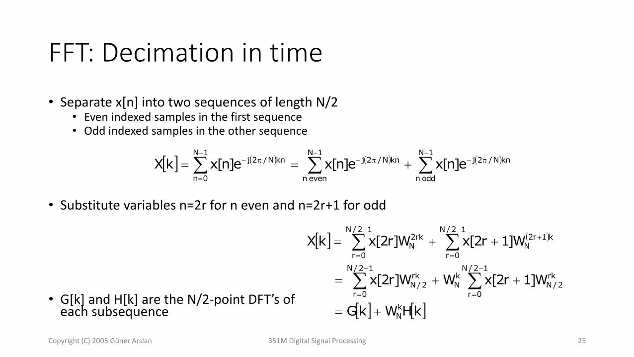
FFT: Decimation in time
24© Prof. I. Selesnick
FFT: Decimation in time
• Separate x[n] into two sequences of length N/2• Even indexed samples in the first sequence• Odd indexed samples in the other sequence
• Substitute variables n=2r for n even and n=2r+1 for odd
• G[k] and H[k] are the N/2-point DFT’s of each subsequence
Copyright (C) 2005 Güner Arslan 351M Digital Signal Processing 25
1N
odd n
knN/2j1N
even n
knN/2j1N
0n
knN/2j e]n[xe]n[xe]n[xkX
kHWkG
W]1r2[xWW]r2[x
W]1r2[xW]r2[xkX
kN
12/N
0r
rk2/N
kN
12/N
0r
rk2/N
12/N
0r
k1r2N
12/N
0r
rk2N
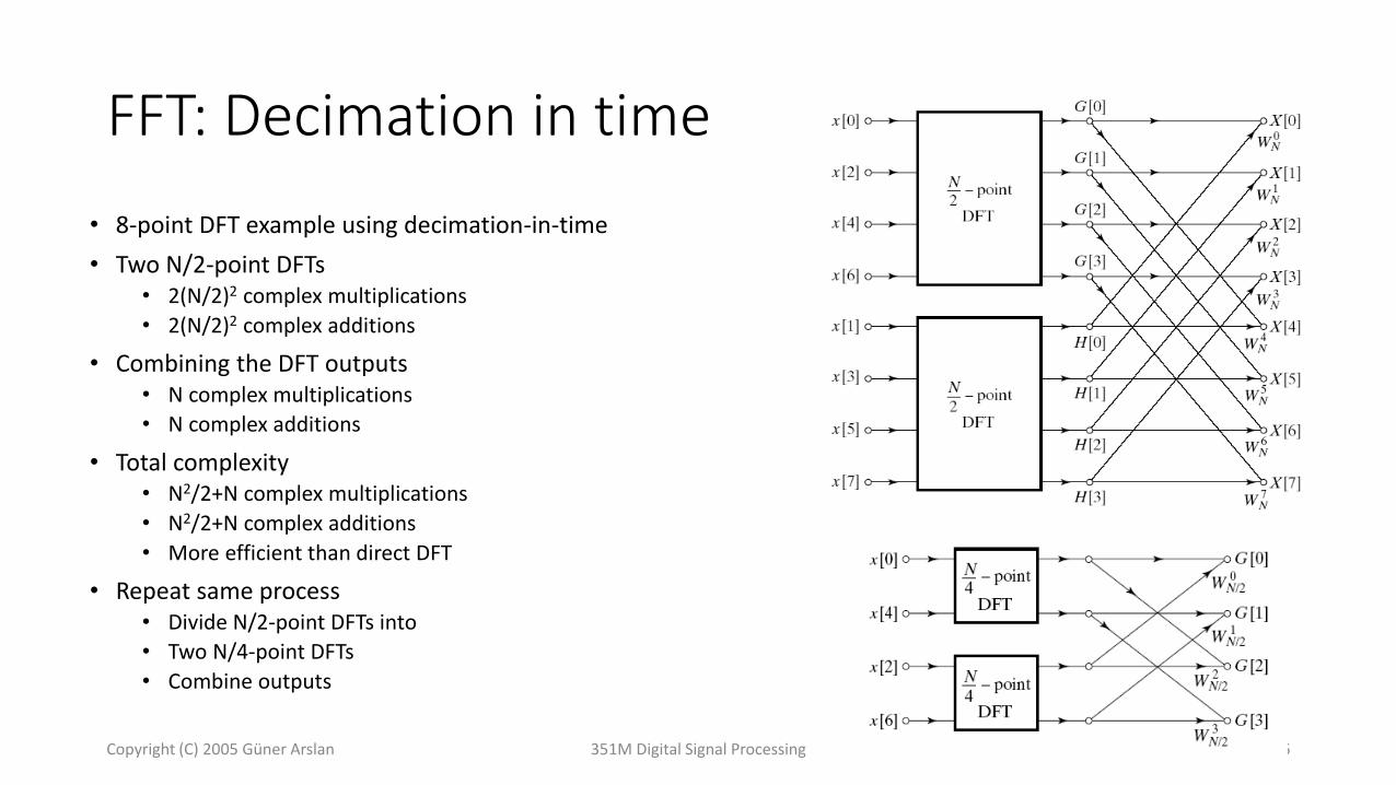
FFT: Decimation in time
Copyright (C) 2005 Güner Arslan 351M Digital Signal Processing 26
• 8-point DFT example using decimation-in-time
• Two N/2-point DFTs• 2(N/2)2 complex multiplications
• 2(N/2)2 complex additions
• Combining the DFT outputs• N complex multiplications
• N complex additions
• Total complexity• N2/2+N complex multiplications
• N2/2+N complex additions
• More efficient than direct DFT
• Repeat same process • Divide N/2-point DFTs into
• Two N/4-point DFTs
• Combine outputs

FFT: Decimation in time
Copyright (C) 2005 Güner Arslan 351M Digital Signal Processing 27
• After two steps of decimation in time
• Repeat until we’re left with two-point DFT’s
• Butterfly structure
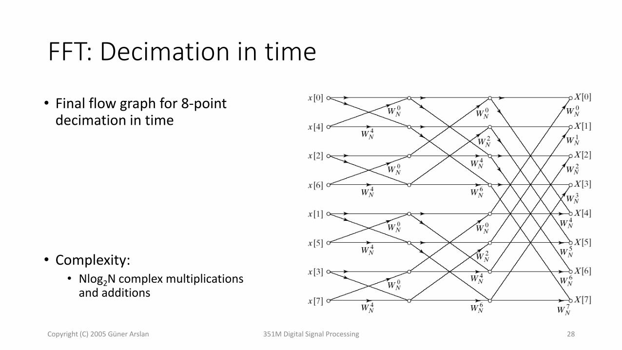
FFT: Decimation in time
Copyright (C) 2005 Güner Arslan 351M Digital Signal Processing 28
• Final flow graph for 8-point decimation in time
• Complexity:• Nlog2N complex multiplications
and additions
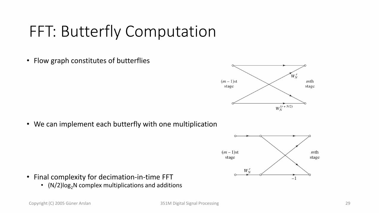
FFT: Butterfly Computation
Copyright (C) 2005 Güner Arslan 351M Digital Signal Processing 29
• Flow graph constitutes of butterflies
• We can implement each butterfly with one multiplication
• Final complexity for decimation-in-time FFT• (N/2)log2N complex multiplications and additions

FFT: In-Place Computation
Copyright (C) 2005 Güner Arslan 351M Digital Signal Processing 30
• Note the arrangement of the input indices to allow in-place computation• Input is overwritten by the output. no auxiliary data structure.
• One physical register needed for both input and output
• Bit reversed indexing
111x111X7x7X
011x110X3x6X
101x101X5x5X
001x100X1x4X
110x011X6x3X
010x010X2x2X
100x001X4x1X
000x000X0x0X
00
00
00
00
00
00
00
00

FFT: Decimation in frequency
• The DFT equation
• Split the DFT equation into even and odd frequency indexes
• Substitute variables to get
• Similarly for odd-numbered frequencies
Copyright (C) 2005 Güner Arslan 351M Digital Signal Processing 31
1N
0n
nkNW]n[xkX
1N
2/Nn
r2nN
12/N
0n
r2nN
1N
0n
r2nN W]n[xW]n[xW]n[xr2X
12/N
0n
nr2/N
12/N
0n
r22/NnN
12/N
0n
r2nN W]2/Nn[x]n[xW]2/Nn[xW]n[xr2X
12/N
0n
1r2n2/NW]2/Nn[x]n[x1r2X
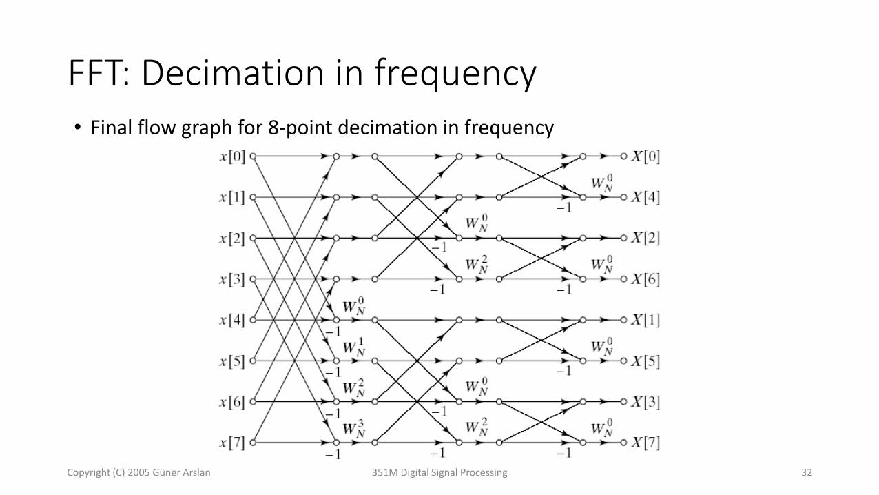
FFT: Decimation in frequency
Copyright (C) 2005 Güner Arslan 351M Digital Signal Processing 32
• Final flow graph for 8-point decimation in frequency

Complexity: FFT vs direct DFT
33

LTI system analysis using FFT
• Short impulse response h[n]
• Very long signal x[n]
34

LTI system analysis using FFT
• Important application when filtering long signals
• Signal x(n) of length L if filtered with FIR filter with impulse response of length M.
• Output is given by a convolution
1
0
)()()(M
m
mnxmhny
• y(n) is of length L+M-1
• To find y(n) it is enough to applyDFT of length: N L+M-1
• Both h and u need to be zero-padded to length N)()()( kXkHkY

L L L
x1(n)
M-1 zeros
x2(n)
M-1 zeros
x3(n)
M-1 zeros
LTI system analysis using FFT: Overlap and add
LTI system analysis using FFT: Overlap and add
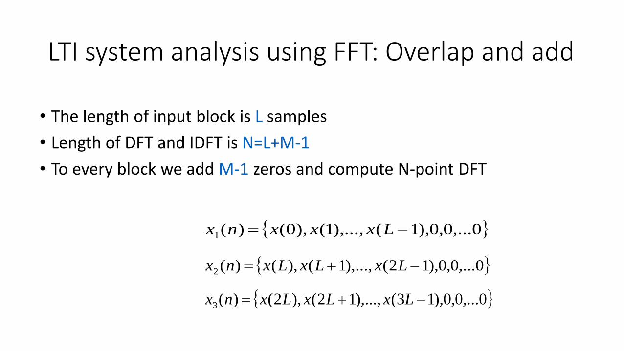
• The length of input block is L samples
• Length of DFT and IDFT is N=L+M-1
• To every block we add M-1 zeros and compute N-point DFT
0,...0,0),1(),...,1(),0()(1 Lxxxnx
0,...0,0),12(),...,1(),()(2 LxLxLxnx
0,...0,0),13(),...,12(),2()(3 LxLxLxnx

LTI system analysis using FFT: Overlap and add
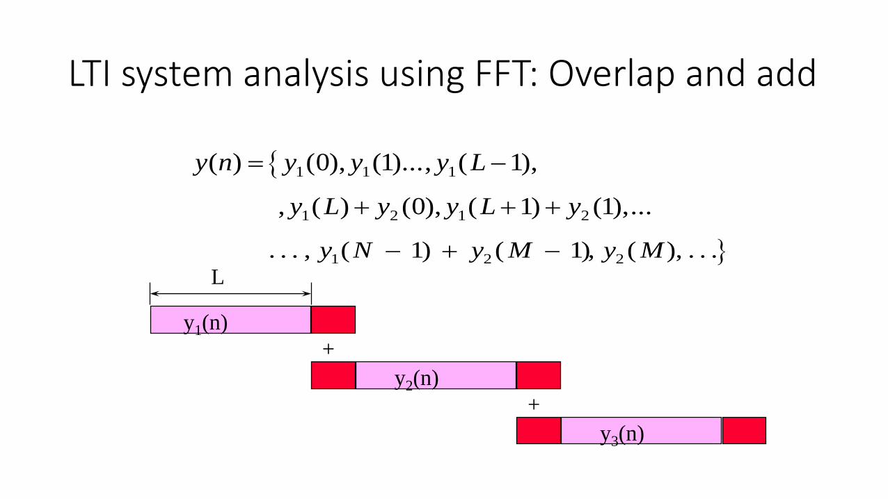
• Ym(k)=H(k)Xm(k) k=0,1,…,N-1
• We obtain output blocks of N where there is no aliasing as the length of DFT-a (IDFT) is N=L+M-1
• We need to overlap the last M-1 samples of each output block with the first M-1 samples of the next block
y1(n)
L
+
y n y y y L( ) ( ), ( )..., ( ), 1 1 10 1 1
y2(n)
, ( ) ( ), ( ) ( ),...y L y y L y1 2 1 20 1 1
+
. . . , ( ) ( )y N y M1 21 1
y3(n)
, ( ), . . .y M2
LTI system analysis using FFT: Overlap and add

LTI system analysis using FFT
• To apply FFT with radix-2 the length of the input block L has to beadjusted so that N (N=L+M-1) is exponent of 2
• Signals x(n) and h(n) have to be zero padded to the lenght of N
• Transformation H(k) of the impulse response is performed only onceas it is time-invariant.

LTI system analysis using FFT
• Block convolution: “overlap and add”
• Input is split into non-overlapping segments
• Perform linear convolution• Need for zero-padding (P-1 zeros)
• Overlap at output: • last P-1 samples of the previous output segment
are added to the current segment
41

• H(k) is computed only once so it can be neglected
• Every FFT needs multiplications
• We perform two of them: 1 x DFT and 1 x IDFT
• To compute Ym(k) we further need N complex multiplications
N N N
N M
N
M
log log2 2 1
• Ratio of number of multiplications by filteringwith FFT vs. linear convolution
log2 1024 1
128
11
128
• E.g. for N=1024 i M=128
LTI system analysis using FFT: Complexity
( / ) logN N2 2
43© Prof. Dennis Freeman, MIT 2011.

44© Prof. Dennis Freeman, MIT 2011.

45© Prof. Dennis Freeman, MIT 2011.

46© Prof. Dennis Freeman, MIT 2011.

47© Prof. Dennis Freeman, MIT 2011.
48© Prof. Dennis Freeman, MIT 2011.