03 Cluster and Factor Analysis
39
Slide 1 Cluster Analysis & Factor Analysis 325-711 Research Methods 2007 Lecturer: Jeromy Anglim Email: [email protected] .au Office: Room 1110 Redmond Barry Building Website: http://jeromyanglim.googlepages.com/ Appointments: For appointments regarding course or with the application of statistics to your thesis, just send me an email “Of particular concern is the fairly routine use of a variation of exploratory factor analysis wherein the researche r uses principal components analysis (PCA), retains components with eigenvalu es greater than 1 and uses varimax rotation, a bundle of procedures affectionately termed “Little Jiffy” …” Preacher, K. J., MacCallum, R. C. (2003). Repairing Tom Swift's Electric Factor Analysis Machine. Understanding Statistics, 2(1), 13-43. DECRIPTION: This session will first introduce student s to factor analysis techniques including common factor analysis and principal components analysis. A factor analysis is a data reduction technique to summarize a number of original variables into a smaller set of composite dimensions, or factors. It is an important step in scale development and can be used to demonstrate construct validity of scale items. We will then move onto cluster analysis techniques. Cluster analysis groups individuals or objects into clusters so that objects in the same cluster are homogeneous and there is heterogeneity across clusters. This technique is often used to segment the data into similar, natural, groupings. For both analytical techniques, a focus will be on when to use the analytical technique, making reasone d decisions about options within each technique, and how to interpret the SPSS output. Slide 2 Overview • Factor Analysis & Principal Components Analysis • Cluster Analysis – Hierarchical – K-means
-
Upload
vimalprajapati -
Category
Documents
-
view
220 -
download
0
Transcript of 03 Cluster and Factor Analysis

8/14/2019 03 Cluster and Factor Analysis
http://slidepdf.com/reader/full/03-cluster-and-factor-analysis 1/39
Slide 1
Cluster Analysis & Factor Analysis
325-711 Research Methods
2007
Lecturer: Jeromy Anglim
Email: [email protected]
Office: Room 1110 Redmond Barry Building
Website: http://jeromyanglim.googlepages.com/
Appointments: For appointments regarding course or with the
application of statistics to your thesis, just send me an email
“Of particular concern is the fairly routine use of a variation ofexploratory factor analysis wherein the researcher usesprincipal components analysis (PCA), retains componentswith eigenvalues greater than 1 and uses varimax rotation, a
bundle of procedures affectionately termed “Little Jiffy” …”Preacher, K. J., MacCallum, R. C. (2003). Repairing Tom Swift's Electric Factor Analysis Machine. UnderstandingStatistics, 2(1), 13-43.
DECRIPTION:
This session will first introduce students to factor analysis techniques including common
factor analysis and principal components analysis. A factor analysis is a data reduction
technique to summarize a number of original variables into a smaller set of composite
dimensions, or factors. It is an important step in scale development and can be used to
demonstrate construct validity of scale items. We will then move onto cluster analysis
techniques. Cluster analysis groups individuals or objects into clusters so that objects in the
same cluster are homogeneous and there is heterogeneity across clusters. This technique is
often used to segment the data into similar, natural, groupings. For both analyticaltechniques, a focus will be on when to use the analytical technique, making reasoned
decisions about options within each technique, and how to interpret the SPSS output.
Slide 2
Overview
• Factor Analysis & Principal
Components Analysis
• Cluster Analysis
–Hierarchical
–K-means

8/14/2019 03 Cluster and Factor Analysis
http://slidepdf.com/reader/full/03-cluster-and-factor-analysis 2/39
Slide 3
Readings
• Tabachnick, B. G., & Fiddel, L. S. (1996). Using Multivariate Statistics. NY:
Harper Collins (or later edition). Chapter 13 Principal Components Analysis
& Factor Analysis.
• Hair, J. F., Black, W. C., Babin, B. J., Anderson, R. E., & Tatham, R. L. ( 2006).
Multivariate Data Analysis (6th ed). New York: Macmillion Publishing
Company. Chapter 8: Cluster Analysis
• Preacher, K. J., MacCallum, R. C. (2003). Repairing Tom Swift's
Electric Factor Analysis Machine. Understanding Statistics,
2(1), 13-43.
• Comrey, A. L. (1988). Factor analytic methods of scale
development in personality and clinical psychology. Journal of
Consulting and Clinical Psychology, 56(5), 754-761.
Tabachnick & Fiddel (1996) The style of this chapter is typical of Tabachnick & Fiddel. It is
quite comprehensive and provides many citations to other authors regarding particular
techniques. It goes through the issues and assumptions thoroughly. It provides advice on
write-up and computer output interpretation. It even has the underlying matrix algebra,
which most of us tend to skip over, but is there if you want to get a deeper understanding.
There is a more recent version of the book that might also be worth checking out.
Hair et al (2006) The chapter is an excellent place to start for understanding factor analysis.
The examples are firmly grounded in a business context. The pedagogical strategies for
explaining the ideas of cluster analysis are excellent.
Preacher & MacCallum (2003) This article calls on researchers to think about the choices
inherent in carrying out a principal components analysis/factor analysis. It criticises the
conventional use of what is called little Jiffy – PCA , eigenvalues over 1, varimax rotation –
and sets out alternative decision rules. In particular it emphasises the importance of making
reasoned statistical decisions and not just relying on default options in statistical packages.
Comrey (1988) Although this is written for the field of personality and clinical psychology, it
has relevance for any scale development process. It offers many practical recommendations
about developing a reliable and valid scale including issues of construct definition, scale
length, item writing, choice or response scales and methods of refining the scale through
factor analysis. If you are going to be developing any form of scale or self-report measure, I
would consider reading this article or something equivalent to be essential. I have seenmany students and consultants in the real world attempt to develop a scale without
internalising the advice in this paper and other similar papers. The result: a poor scale…
Before we can test a theory using empirical methods, we need to sort issues of
measurement.
8/14/2019 03 Cluster and Factor Analysis
http://slidepdf.com/reader/full/03-cluster-and-factor-analysis 3/39
Slide 4
Motivating Questions
• How can we explore structure in our dataset?
• How can we reduce complexity and see the
pattern?
• Group many cases into groups of cases?
• Group many variables into groups of
variables?
Slide 5
Purpose of factor analysis
• Latent factors (Factor Analysis)
– Uncover latent factors underlying a set of variables
• Variable reduction (Principal Component Analysis)
– Reduce a set of variables to a smaller number, while stillaccounting for “most” of the variance
• Examples
– Test/scale construction
– Data reduction
– Variables created often used in subsequent
analyses
Factor Analysis and Principal Components Analysis are both used to reduce a large set of
items to a smaller number of dimensions and components. These techniques are commonly
used when developing a questionnaire to see the relationship between the items in thequestionnaire and underlying dimensions. It is also used in general to reduce a larger set of
variables to a smaller set of variables that explain the important dimensions of variability.
Specifically, Factor analysis aims to find underlying latent factors, whereas principal
components analysis aims to summarise observed variability by a smaller number of
components.

8/14/2019 03 Cluster and Factor Analysis
http://slidepdf.com/reader/full/03-cluster-and-factor-analysis 4/39
Slide 6
When have I used this technique?
• Employee Opinion Surveys
• Market Research
• Test Construction
• Experimental Research
• Consulting for others
Employee Opinion Surveys: Employee opinion surveys commonly have 50 to 100 questions
relating to the employee’s perception of their workplace. These are typically measured on a
5 or 7 point likert scale. Questions can be structured under topics such as satisfaction with
immediate supervisor, satisfaction with pay and benefits, or employee engagement. While
individual items are typically reported to the client, it is useful to be able to communicate
the big picture in terms of employee satisfaction with various facets of the organisation.
Factor analysis can be used to guide the process of grouping items into facets or to check
that the proposed grouping structure is consistent with the data. The best factor structures
are typically achieved when the items were designed with a specific factor structure in mind.
However, designing with an explicit factor structure in mind may not be consistent with
managerial desire to include specific questions.
Market research: In market research customers are frequently asked about their satisfaction
with a product. Satisfaction with particular elements is often grouped under facets such as
price, quality, packaging, etc. Factor analysis provides a way of verifying the appropriateness
of the proposed facet grouping structure. I have also used it to reduce large number of
correlated items to a smaller set in order to use the smaller set as predictors in a multiple
regression.
Experimental Research: I have often developed self-report measures based on a series of
questions. Exploratory factor analysis was used to determine which items are measuring a
similar construct. These items were then aggregated to form an overall measure of theconstruct, which could then be in used in subsequent analyses.
Test Construction: When developing ability, personality or other tests, the set of test items is
typically broken up in to sets of items that aim to measure particular subscales. Factor
analysis is an important process assessing the appropriateness of proposed subscales. If you
are developing a scale, exploratory factor analysis is very important in developing your test.
Although researchers are frequently talking about confirmatory factor analysis using
structural equation modelling software to validate their scales, I tend to think that in the
development phase of an instrument exploratory factor analysis tends to be more useful in
making recommendations for scale improvement.

8/14/2019 03 Cluster and Factor Analysis
http://slidepdf.com/reader/full/03-cluster-and-factor-analysis 5/39
Slide 7
Sorting out language
• Most of the rules around interpretation of
principal components analysis and factor
analysis are the same
• The underlying mathematical models and
theoretical purposes are distinct
• In order not to present everything twice, the
word components and factors are used
interchangeably
Slide 8
An Introductory Example
• Theory suggests the 9 ability tests reflect 3
underlying ability factors, does the data
support this claim?

8/14/2019 03 Cluster and Factor Analysis
http://slidepdf.com/reader/full/03-cluster-and-factor-analysis 6/39
Slide 9
Descriptive Statistics
• What can you learn about the variables from looking atthis table?
Descriptive Statistics
.30 .24 112
.59 .21 112
.33 .17 112
21.36 4.14 112
10.86 2.63 112
8.71 1.99 112
223.38 39.20 112
290.32 51.52 112
398.63 91.82 112
GA: Cube Comparison - Total Score ([correct - incorrect] / 42)
GA: Inference - Total Score ([correct - .25 incorrect] / 20)
GA: Vocabulary- Total Score ([correct - .25 incorrect] / 48)
PSA: Clerical Speed Total (Average Problems Solved [Correct -Incorrect] per minute)
PSA: Number Sort (Average Problems Solved (Correct - Incorrect)per minute)
PSA: Number Comparison (Average Problems Solved (Correct -Incorrect) per minute)
PMA: Simple RT Average (ms)
PMA: 2 Choice RT Average (ms)
PMA: 4 Choice RT (ms)
Mean S td. Devi at i on A na lysi s N
Slide 10
Communalities
1.000 .291
1.000 .826
1.000 .789
1.000 .706
1.000 .724
1.000 .727
1.000 .782
1.000 .867
1.000 .844
GA: Cube Comparison - Total Score ([correct - incorrect] / 42)
GA: Inference - Total Score ([correct - .25 incorrect] / 20)
GA: Vocabulary- Total Score ([correct - .25 incorrect] / 48)
PSA: Clerical Speed Total (Average Problems Solved [Correct - Incorrect] per minute)
PSA: Number Sort (Average Problems Solved (Correct - Incorrect) per minutePSA: Number Comparison (Average Problems Solved (Correct - Incorrect) peminute)
PMA: Simple RT Average (ms)
PMA: 2 Choice RT Average (ms)
PMA: 4 Choice RT (ms)
Init ia l Ex tr ac ti on
Extraction Method: Principal Component Analysis.
Communalities
After extracting 3 components
• Which variables have less than half their variance explained by the 3components extracted?
• Cube Comparison Test
• Conclusion: This test may be unreliable or may be measuringsomething quite different to the other tests
• Might consider dropping it

8/14/2019 03 Cluster and Factor Analysis
http://slidepdf.com/reader/full/03-cluster-and-factor-analysis 7/39
Slide 11
How many components to extract?
• Theory says: 3 components
• Eigenvalues over 1 says: 3 components
• Scree plot: unclear – 2, 3 or 4 seem plausible
• Decision: I‟ll go with 3 because it is consistent with
theory and is at least not „inconsistent‟ with the scree plot
Where does the screestart?
Slide 12
1.1 Variance Explained by the three
componentsTotal Variance Explained
3.827 42.520 42.520 3.827 42.520 42.520 3.155
1.649 18.324 60.844 1.649 18.324 60.844 3.042
1.080 12.003 72.847 1.080 12.003 72.847 1.966
.849 9.437 82.283
.490 5.443 87.726
.373 4.147 91.873
.318 3.535 95.407
.279 3.101 98.508
.134 1.492 100.000
Component1
2
3
45
6
7
8
9
Total % of Varian ce Cum ulative % Tota l % o f Varianc e Cum ulative % Tota l
Init ia l E igen values E xt rac tion S ums of Square d Load ings Rotation
Extraction Method: Principal Component Analysis.
When components are correlated, sums of squared loadings cannot be added to obtain a total variance.a.
How much variance is explained by the three components?
Prior to rotation how evenly is the variance distributed across the
three components?
What about after an oblique rotation?
How much variance is explained by the three components?
Prior to rotation how evenly is the variance distributed across the three components?
What about after an oblique rotation?

8/14/2019 03 Cluster and Factor Analysis
http://slidepdf.com/reader/full/03-cluster-and-factor-analysis 8/39
Slide 13
Component Matrixa
.498 .204 .036
.609 .564 -.370
.257 .736 -.425
.677 -.097 .488
.677 .319 .405
.694 .283 .407
-.742 .369 .309
-.770 .467 .238
-.775 .449 .204
GA: Cube Comparison - Total Score ([correct - incorrect] / 42)
GA: Inference - Total Score ([correct - .25 incorrect] / 20)
GA: Vocabulary- Total Score ([correct - .25 incorrect] / 48)
PSA: Clerical Speed Total (Average Problems S olved [Correct -Incorrect] per minute)
PSA: Number Sort (Average Problems S olved (Correct -Incorrect) per minute)
PSA: Number Comparison (Average Problems Solved (Correct -Incorrect) per minute)
PMA: Simple RT Average (ms)
PMA: 2 Choice RT Average (ms)
PMA: 4 Choice RT (ms)
1 2 3
Component
Extraction Method: Principal Component Analysis.
3 components extracted.a.
Interpreting Unrotated solution
What does each component mean?
What does each component mean?1st Component (‘g’): Reflects Ability on all tests, but vocab less important2nd Component (Intelligent, but slow): Vocabulary, inference and being slow on RTtests3rd Component (‘fast on paper ’): High perceptual speed, slow RT and poor vocaband inference
Slide 14
Pattern Matrixa
-.113 .353 .237
-.176 .113 .816
.118 -.063 .911
-.144 .805 -.266
.109 .857 .110
.074 .855 .085
.898 .065 -.089
.940 .010 .031
.907 -.033 .039
GA: Cube Comparison - Total Score ([correct - incorrect] / 42)
GA: Inference - Total Score ([correct - .25 incorrect] / 20)
GA: Vocabulary- Total Score ([correct - .25 incorrect] / 48)
PSA: Clerical Speed Total (Average Problems Solved [Correct -Incorrect] per minute)
PSA: Number Sort (Average Problems Solved (Correct - Incorrect) per minute)
PSA: Number Comparison (Average Problems Solved (Correct -Incorrect) per minute)
PMA: Simple RT Average (ms)
PMA: 2 Choice RT Average (ms)
PMA: 4 Choice RT (ms)
1 2 3
Component
Extraction Method: Principal Component Analysis.Rotation Method: Promax with Kaiser Normalization.
Rotation converged in 5 iterations.a.
Interpreting Oblique Rotated Solution
Component Correlation Matrix
1.000 -.475 -.143-.475 1.000 .309
-.143 .309 1.000
Component
12
3
1 2 3
Extraction Method: Principal Component Analysis.Rotation Method: Promax with Kaiser Normalization.
What does each of the components measure?1st Components: Psychomotor Ability (PMA)2nd Component: Perceptual Speed Ability (PSA)3rd Component: General Ability (GA)Answering Research Question: Convergence with theory / Problematic items?
Pretty good, but Cube comparison did not load on General Ability as
anticipated; It does not load much on anything, but if anything it is morerelated to perceptual speed ability

8/14/2019 03 Cluster and Factor Analysis
http://slidepdf.com/reader/full/03-cluster-and-factor-analysis 9/39
What is the correlation between Components?1 (PMA) with 2 (PSA) is strongest; 2 (PSA) with 3 (GA) is moderate.Note: oblique rotation chosen because different abilities are assumed theoretically to be
correlated; this is supported by the component correlation matrix
Slide 15
Correlation• Factor Analysis is only as good as your correlation
matrix
– Sample size
– Linearity
– Size
r 50 100 150 200 250 300 350 400 450 500
0 .28 .20 .16 .14 .12 .11 .10 .10 .09 .090.3 .26 .18 .15 .13 .11 .10 .10 .09 .08 .080.5 .21 .15 .12 .10 .09 .09 .08 .07 .07 .070.8 .11 .07 .06 .05 .05 .04 .04 .04 .03 .03
Sample Size
Given an obtained correlation and sample size, 95% confidence intervalsare approximately plus or minus the amount shown in cellse.g., r=.5, n=200, CI95% is .09; i.e., population correlation approximatelyranges between .41 and .59 (95% CI)Estimates derived from Thomas D. Fletcher „s CIr function in R – psychometrics package
In general terms factor analysis and principal components analysis are concerned with
modelling the correlation matrix. Factor analysis is only as good as the correlations are that
make it up.
SAMPLE SIZE: Larger sample sizes make correlations more reliable estimates of the
population correlation. This is why we need reasonable sample sizes. If we look at the tableabove we see that our estimates of population correlations get more accurate as the sample
size increases and as the size of the correlation increases. Note that technically confidence
intervals around correlations are asymmetric. The main point of the table is to train your
intuition regarding how confident we can be about the population size of a correlation.
When confidence 95% confidence intervals are in the vicinity of plus or minus .2, there is
going to be a lot of noise in the correlation matrix, and it may be difficult to discern the true
population structure.
VARIABLE DISTRIBUTIONS: Skewed data or data with insufficient scale points can lead to
attenuation of correlations between measured variables versus the underlying latent
constructs of the items.LINEARITY: If there are non-linear relationships between variables, then use of the pearson
correlation which assesses only the linear relationship will be misleading. This can be
checked my examination of matrix scatterplot between variables.
SIZE OF CORRELATIONS: If the correlations between the variables tend to all be low (e.g., all
less than .3), factor analysis is likely to be inappropriate because speaking about variables in
common when there is no common variance makes little sense.
INTUITIVE UNDERSTANDING: It can be a useful exercise in gaining a richer understanding of
factor analysis to examine the correlation matrix. You can circle medium (around .3), large
(around .5) and very large (around .7) correlations and think about how such items are likely
to group together to form factors.
8/14/2019 03 Cluster and Factor Analysis
http://slidepdf.com/reader/full/03-cluster-and-factor-analysis 10/39
Slide 16
Polychoric correlations
• Polychoric Correlation
– Estimate of correlation between assumed
underlying continuous variables of two ordinal
variables
• Also see Tetrachoric correlation
• Solves
– Items factoring together because of similar
distributions
http://ourworld.compuserve.com/homepages/jsuebersax/tetra.htm
This technique is not available in SPSS. Although if you are able to compute a polychoric
correlation matrix in another program, this correlation matrix can then be analysed in SPSS.
The above website lists software that implements the technique. R is the program that I
would use to produce the polychoric correlation matrix.
This is the recommended way of factor analysing test items on ordinal scales, such as the
typical 4, 5 or 7 point scales. From my experience these are the most common applications
of factor analysis, such as when developing surveys or other self-report instruments.
The tetrachoric correlation is used to estimate correlations between binary items when
there is assumed to be an underlying continuous variable.
This technique has also more general relevance to situations where you are correlating
ordinal variables with an assumed ordinal distributions.
One of my favourite articles on the dispositional effects of job satisfaction (Staw & Ross,
1985) using a sample of 5,000 men measured five years apart found that of those who had
changed occupations and employers, there was still a job satisfaction correlation of .19 over
the five years. However, this was based on a single job satisfaction item measured on a four
point scale. Having just a single item on a four point scale would attenuate the true
correlation. Thus, using the polychoric correlation, an estimate could be made of the
correlation of job satisfaction in the continuous sense over time.
Staw, B. M., & Ross, J. (1985). Stability in the midst of change: A dispositional approach to job attitudes. Journal of Applied Psychology, 70, 469-480.

8/14/2019 03 Cluster and Factor Analysis
http://slidepdf.com/reader/full/03-cluster-and-factor-analysis 11/39
Slide 17
Communalities• Simple conceptual definition
– Communality tells us how much a variable has “incommon” with the extracted components
• Technical definition
– Percentage of variance explained in an variable bythe extracted components
• Why we care?
• Practical interpretation
– Jeromy‟s rules of thumb:
• <.1 is extremely low; <.2 is very low; <.4 is low; <.5 issomewhat low
– Compare relative to other items in the set
Communalities: Communalities represent the percentage of variance explained by the
extracted components.
If you were to run a regression predicting the item from the extracted components, the
communality would be the r-squared.
If you square the unrotated loadings for an item for each of the components and sum these,
you get the communality.
Why we care: If the communality is very low for an item, it suggests that it does not share
much in common with the extracted components. This generally implies that it is unrelated
to the other items in the set.
What causes a communality to be low for an item? The basic idea is that anything that
reduces the correlations between the items will tend to
The following are all possible explanations for low communalities with the basic theme
being :
The item was poorly designed (e.g., the item was not understood by respondents)
The item has very little variance, usually resulting from large positive or negative skew (e.g.,
everyone ticks strongly agree)
Within the set of items, it is the only item that aims to measure a particular construct (e.g., a
survey about employee engagement with a single question about pay).
A response scale with a small number of categories. Response scales with 2, 3, 4 or even 5
categories often show attenuated correlations with other variables.What we do about a low communality? An integrated assessment should be made relative
to the how low it the communality and the plausible reasons for the communality and the
role of the variable in the set. We may wish to remove the item from the analysis either to
exclude it from any further analyses or to treat it as a stand alone variable.
It may suggest that in future we should add more items measuring the construct that this
item is aiming to measure.
8/14/2019 03 Cluster and Factor Analysis
http://slidepdf.com/reader/full/03-cluster-and-factor-analysis 12/39
Slide 18
Threats to valid inferences
• Factorability
• Adequate sample size
• Normality
• Linearity
• Metric or binary variables
• Absence of Haywood cases
Factorability See discussion below
Sample Size Factor analysis performs better with big samples. As a general rule, factor
analysis requires a minimum of around 150 participants in order to get a reliable solution. If
correlations between items and the factor loadings are large (e.g., several correlations >.5),
sample size can be less and the opposite if the correlations are low. The more items per
factor, the fewer participants required.
Normality Significance tests used in factor analysis assume variables are univariate, bivariate
and multivariate normally distributed. Factor analytic solutions may also be improved when
normality holds in the data. Normality is not a requirement in order to run a factor analysis.
However, severe violations of normality, such as extreme skew, may make untransformed
correlations a misleading representation of the association between two variables. In
addition, there is a tendency for items with similar distributions to group together in factor
analysis independent
Linearity Factor analysis is based on analyses of correlations and covariances. Correlations
and covariances measure the linear relationship between variables. Linear relationships are
usually the main forms of relationships for the kinds of purposes that factor analysis is
typically applied. If the relationships between variables are non-linear, factor analysis
probably is not an appropriate method.
Variable types Factor analysis can be performed on continuous or binary data. It is often
also performed on what would be described as ordinal data. It is very common to analysesurvey items that are on 5 points scales. Note the earlier recommendation regarding the use
of polychoric correlations in the context of ordinal variables.
Absence of Haywood cases Haywood cases can occur when computational problems arise
when extracting a solution in factor analysis. The main indicator of a Haywood case is an
unrotated factor loading that is very close to one (e.g., .99). When this occurs the solution
provided should not be trusted. A common cause of Haywood cases is the extraction of too
many factors. Thus, a resolution to the problem of Haywood cases is to extract fewer factors.
Another resolution is to try a different method of extraction.

8/14/2019 03 Cluster and Factor Analysis
http://slidepdf.com/reader/full/03-cluster-and-factor-analysis 13/39
Slide 19
Sample Size
– More is better
– Higher communalities (higher correlations
between items) means smaller sample required
– More items per factor means smaller sample
required
– N=200 is a reasonable starting point
• But can usually get something out of less (e.g., N=100)
– Consider your purpose
The larger the sample size, the better. Confidence that results are reflecting true population
processes increases as sample size increases. Thus, there is no one magical number below
which the sample size is too small and above which the sample size is sufficient. It is a
matter of degree.
However, in order to develop your intuition about what sample sizes are good, bad and ugly,
the above rules of thumb can help.
You might want to start with the idea that 200 would be good, but that if some of the
correlations between items tends to be large and/or you have large number of items per
factor, you could still be good with a smaller sample size, such as 100.
The idea is to build up an honest and reasoned argument about the confidence you can put
in your results given your sample size and other factors such as the communalities and item
to factor ratio.
Consider your purpose: If you are trying to develop a new measure of a new construct you
are likely to want a sample size that is going to give you robust results. However, if you are
just checking the factor structure of an existing scale in a way that is only peripheral to your
main research purposes, you may be satisfied with less robust conclusions.

8/14/2019 03 Cluster and Factor Analysis
http://slidepdf.com/reader/full/03-cluster-and-factor-analysis 14/39
Slide 20
Factorability
• Kaiser-Meyer Measure of Sampling Adequacy
– in the .90s marvellous
– in the .80s meritorious
– in the .70s middling
– in the .60s mediocre
– in the .50s miserable
– below .50 unacceptable
• Examination of correlation matrix
• Other diagnostics
MSA: The first issue is whether factor analysis is appropriate for the data. An examination of
the correlation matrix of the variables used should indicate a reasonable number of
correlations of at least medium size (e.g., > .30). A good general summary of the applicability
of the data set for factor analysis is the Measure of Sampling Adequacy (MSA). If MSA is too
low, then factor analysis should not be performed on the data.
SPSS can produce this output.
Correlation Matrix: Make sure there are at least some medium to large correlation (e.g., >.3)
between items.
Slide 21
How many factors?
• The maximum possible factors
• Scree plot
• Eigenvalues over 1
• Parallel test
• MAPS test• RMSEA
• Theory
• Principles of parsimony and practical utility
df NS
df Chisquare RMSEA
)1(
There are several approaches for deciding how many factors to extract. Some approaches
are better than the others. A good general strategy is to determine how many factors are
suggested by the better tests (e.g., scree plot, parallel test, theory). If these different
approaches suggest the same number of factors, then extract this amount. If they suggest
varying numbers of factors, examine solutions with the range of factor suggested and selectthe one that appears most consistent with theory or the most practically useful.

8/14/2019 03 Cluster and Factor Analysis
http://slidepdf.com/reader/full/03-cluster-and-factor-analysis 15/39
Maximum number of factors
Based on the requirement of identification, it is important to have at least three items per
factor. Thus, if you have 7 variables, this would lead to a maximum of 2 factors (7/3 = 2.33,
rounded to 2). This is not a rule for determining how many factors to extract. It is just a rule
about the maximum number of factor to extract.
Scree Plot: The scree plot shows the eigenvalue associated with each component. An
eigenvalue represents the variance explained by each component. An eigenvalue of 1 is
equivalent to the variance of a single variable. Thus, if you obtain an eigenvalue of 4, and
there are 10 variables being analysed, this component would account for 4 / 10 or 40% of
the variance in items. The nature of principal components analysis is that it creates a
weighted linear composite of the observed variables that maximises the variance explained
in the observed variables. It then finds a seconds weighted linear composite which
maximises variance explained in the observed variables, but based on the condition that it
does not correlate with the previous dimension or dimensions. This process leads to each
dimension accounting for progressively less variance. It is typically assumed that there will
be certain number of meaningful dimensions and then a remaining set which just reflectitem specific variability. The scree plot is a plot of the eigenvalues for each component,
which will often show a few meaningful components that have substantially larger
eigenvalues than later components followed which in turn show a slow steady decline. We
can use the scree plot to indicate the number of important or meaningful components to
extract. The point at which the components start a slow and steady decline is the point
where the less important components commence. We go up one from when this starts and
this indicates the number of components to extract.
Looking at the figure below highlights the degree of subjectivity in the process. Often it is
not entirely clear when the steady decline commences. In the figure below, it would appear
that there is a large first component, a moderate 2nd
and 3rd
component, and a slightlysmaller 4
th component. From the 5
th component onwards there is steady gradual decline.
Thus, based on the rule that the 5th
component is the start of the unimportant components,
the rule would recommend extracting 4 components.
Eigenvalues over 1: This is a common rule for deciding how many factors to extract. It
generally will extract too many factors. Thus, while it is the default option in SPSS, it
generally should be avoided.
Parallel Test: The parallel test is not built into SPSS. It requires the downloading of additional
SPSS syntax to run.
http://flash.lakeheadu.ca/~boconno2/nfactors.html
The parallel test compares the obtained eigenvalues with eigenvalues obtained usingrandom data. It tends to perform well in simulations.
MAPS test: This is also available from the above website and is also regarded as good
method for estimating the correct number of components.
RMSEA: When using maximum likelihood factor analysis or generalised least squares factor
analysis, you can obtain a chi square test indicating the degree to which the extracted factors
enable the reproduction of the underlying correlation matrix. RMSEA is a measure of fit
based on the chi-square value and the degrees of freedom. One rule of thumb is to take the
number of factors with the lowest RMSEA or the smallest number of factors that has an
adequate RMSEA. In SPSS, you need to manually calculate it. Browne and Cudeck (1993)
have suggested rules of thumb: RMSEA >0.05 – close fit; between 0.05 and 0.08 – fair fit;between 0.08 and 0.10 – mediocre fit, and; >0.10 – unacceptable fit.

8/14/2019 03 Cluster and Factor Analysis
http://slidepdf.com/reader/full/03-cluster-and-factor-analysis 16/39
Theory & Practical Utility
Based on knowledge of the content of the variables, a researcher may have theoretical
expectations about how many factors will be present in the data file. This is an important
consideration. Equally, researchers differ in whether they are trying to simplify the story or
present all the complexity.
Slide 22
Eigenvalues over 1
• Default rule of thumb in SPSS
• Rationale: a component should account for
more variance than a variable to be
considered relevant
• Generally considered to recommend too many
components particularly when sample sizes
are small or the number of items to
components is large
Slide 23
Scree plot.• Why‟s it called a scree plot?
– Scree: The cruddy rocks at the bottom of a cliff
– How many factors?• “We don‟t want the crud; we want the mighty cliff; so we go up
one from where the scree starts”
To make the idea of scree really concrete, check out the article and learn something about
rocks and mountains in the process
http://en.wikipedia.org/wiki/Scree
8/14/2019 03 Cluster and Factor Analysis
http://slidepdf.com/reader/full/03-cluster-and-factor-analysis 17/39
Slide 24
How many factors? The final decision
• Criteria1. Scree plot
2. Eigenvalues over 1
3. Parallel test
4. MAPS test
5. RMSEA
6. Theory
7. Principles of
parsimony and
practical utility
8. There’s more
• Final decision – Know
• Know how manycomponents each criteriasuggests
– Assess applicability
• Weight criteria by itsapplicability
– Decide
• Make a reasoned decisionintegrating the above twopoints
This is a really important decision in factor analysis and it is important to provide agood reasoned explanation for the particular decision adopted.
Slide 25
Extraction Methods
• Principal Components Analysis
• True Factor Analysis
– Maximum Likelihood
– Generalised Least Squares
– Unweighted Least Squares
Principal Components Analysis uses a different mathematical procedure to factor analysis.Factor analysis extraction methods in SPSS include: Maximum Likelihood, Generalised Least
Squares, and Unweighted Least Squares.
The most established is Maximum Likelihood and it is the one recommended for most
contexts.
If you are curious, try your analysis with different extraction methods and see what effect it
has on your substantive interpretation. Frequently in practice, the method of extraction does
not make much difference in the results achieved.
If you are interested in extracting underlying factors, it would make more sense to use a true
factor analytic method, such as Maximum Likelihood. If you want to create a weighted
composite of existing variables, principal components may be the more appropriate method.

8/14/2019 03 Cluster and Factor Analysis
http://slidepdf.com/reader/full/03-cluster-and-factor-analysis 18/39
Slide 26
Logic of Principal Components
Analysis
• More precisely: – Extract a weighted sum of the variables where
the weights are chosen to maximise thevariance explained in the variables
– Repeat for second and subsequentcomponents, making sure that they areuncorrelated with prior components
Breaking the Name down:
Note that its not “principle”; it’s “principal”
Principal “First, highest, or foremost in importance, rank, worth, or degree; chief” – Answers.com
Component “A constituent element, as of a system” – Answers.com
Slide 27
A little matrix algebra• Terms
– Matrix: A table (rows and columns) of values
– Vector: A single column or row of values
– Scalar: A single value
– Eigenvalue: Sum of variance in variables explained bycomponent
– Eigenvector: A column of numbers representingcorrelation between a component and each variable
• Principal Components Analysis Equation
R = VLV΄
R = Correlation Matrix of variables
L = Diagonal matrix of eigenvalues for all components
V = Matrix made up of as many Eigenvectors as
components
Advice on Matrix Algebra
Most multivariate procedures are solved using matrix algebra. Multivariate statistics also involves a
large number of matrices.
Knowing a little matrix algebra can help you better understand the world of multivariate statistics.
Getting familiar with the basic terms is worthwhile. The more you learn, the deeper you can take the
techniques.
If you want to learn more:
A great ebook: http://numericalmethods.eng.usf.edu/matrixalgebrabook/frmMatrixDL.asp
Tabachnick & Fiddel have an Appendix
If you decide to learn R, learning matrix algebra becomes a lot easier. This tutorial is quite good:http://personality-project.org/r/sem.appendix.1.pdf

8/14/2019 03 Cluster and Factor Analysis
http://slidepdf.com/reader/full/03-cluster-and-factor-analysis 19/39
Matrix: A table (rows and columns) of values
Some of the most common matrices encountered in multivariate statistics include:
Dataset: columns represent variables and rows represent cases.
Correlation (or covariance or Sums of Squares and Crossproducts [SSCP]) matrix: A square matrix
where the same variables are in the rows and columns and the cells represent correlations (or
covariance or SSCP) between variablesVector: A single column or row of values
Common examples include:
Data on a single variable (i.e., the value of a particular variable for a series of cases)
Weights for a set of variables: In principal components analysis, multiple regression and other
techniques, scores are produces by multiplying a set of variables by a set of weights. These weights
can be recorded as a vector.
Scalar: A single value
Eigenvalue: Sum of variance in variables explained by component
Eigenvector: A column of numbers representing correlation between a component and each variable
Slide 28
Variance Explained• Variance Explained
– Eigenvalues
– % of Variance Explained
– Cumulative % Variance Explained
• Initial, Extracted, Rotated
• Why we care?
– Practical importance of a component is related toamount of variance explained
– Indicates how effective we have been in reducingcomplexity while still explaining a large amount ofvariance in the variables
– Shows how variance is re-distributed after rotation
Eigenvalue:
The average variance explained in the items by a component multiplied by the number of
components.
An eigenvalue of 1 is equivalent to the variance of 1 item.
% of variance explainedThis represent the percentage of total variance in the items explained by a component.
This is equivalent to the eigenvalue divided by the number of items.
This is equivalent to the average item communality for the component.
8/14/2019 03 Cluster and Factor Analysis
http://slidepdf.com/reader/full/03-cluster-and-factor-analysis 20/39
Slide 29
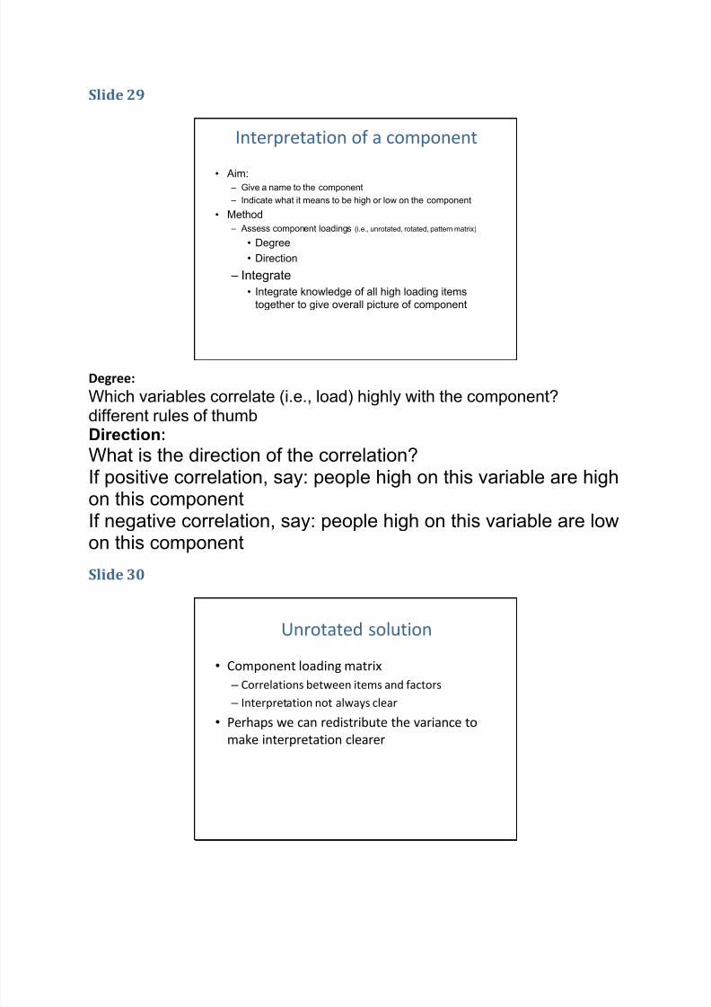
Interpretation of a component
• Aim: – Give a name to the component
– Indicate what it means to be high or low on the component
• Method
– Assess component loadings (i.e., unrotated, rotated, pattern matrix)
• Degree
• Direction
– Integrate
• Integrate knowledge of all high loading itemstogether to give overall picture of component
Degree:
Which variables correlate (i.e., load) highly with the component?different rules of thumbDirection:
What is the direction of the correlation?If positive correlation, say: people high on this variable are highon this component
If negative correlation, say: people high on this variable are lowon this component
Slide 30
Unrotated solution
• Component loading matrix
– Correlations between items and factors
– Interpretation not always clear• Perhaps we can redistribute the variance to
make interpretation clearer

8/14/2019 03 Cluster and Factor Analysis
http://slidepdf.com/reader/full/03-cluster-and-factor-analysis 21/39
Slide 31
Rotation• Basic idea
– Based on idea of actually rotating component axes
• What happens
– Total variance explained does not change
– Redistributes variance over components
• Why do we rotate?
– Improve interpretation by maximising simple structure
• Each variable loading highly on one and only one component
Slide 32
Orthogonal vs Oblique
Rotations• Orthogonal
– Right angles (uncorrelated components)
– Varimax, Quartimax, Equamax
– Interpret: Rotated Component Matrix
– Sum of rotated eigenvalues equals sum of unrotated eigenvalues
• Oblique – Not at right angles (correlated components)
– Direct Oblimin & Promax
– Interpret: Pattern Matrix & Component Correlation Matrix
– Sum of rotated eigenvalues greater than sum of unrotated eigenvalues
• Which type do you use? – Oblique usually makes more conceptual sense
– Generally, oblique rotation better at achieving simple structure
SPSS Options
Rotation serves the purpose of redistributing the variance accounted for by the factors so
that interpretation is clearer. A clear interpretation can generally be conceptualised as each
variable loading highly on one and only one factor.Two broad categories of rotation exist, called oblique and orthogonal.
Orthogonal rotation
Orthogonal rotations in SPSS are Varimax, Quartimax, and Equamax and force factors to be
uncorrelated. These different rotation methods define simple structure in different ways.
Oblique rotations in SPSS are Direct Oblimen and Promax. These allow for correlated factors.
The two oblique rotation methods each have a parameter which can be altered to increase
or decrease the level of correlation between the factors.
The decision on whether to perform an oblique or orthogonal rotation can be influenced by
whether you expect the factors to be correlated.

8/14/2019 03 Cluster and Factor Analysis
http://slidepdf.com/reader/full/03-cluster-and-factor-analysis 22/39
Slide 33
Factor Saved Scores
• Options
– Regression
– Bartlett
• Decision
– Factor saved scores vs creating your own
composites
A typical application of a factor analysis is to see how variables should be grouped together.
Then, a score is calculated for each individual on each factor. And this score is used in
subsequent analyses. For example, you might have a test that measures intelligence and that
it is based on a number of items. You might want to extract a score and use this to predict
job performance.
There are two main ways of creating composites:
• Factor saved scores
• Self created composites
Factor saved scores are easy to generate in SPSS using the factor analysis procedure. They
may also be more reliable measures of the factor, although often they are very highly
correlated with self-created composites
Self-created composites are created by adding up the variables, usually based on those that
load most on a particular factor. In SPSS this is typically done using the Transform >>
Compute command. They can optionally be weighted by their relative importance. The
advantage of self-created composites is that the raw scores are more readily comparable
across studies.

8/14/2019 03 Cluster and Factor Analysis
http://slidepdf.com/reader/full/03-cluster-and-factor-analysis 23/39
Slide 34
Cluster Analysis
• Core Elements
– PROXIMITY: What makes two objects similar?
– CLUSTERING: How do we group objects?
– HOW MANY?: How many groups do we retain?
• Types of cluster analysis
– Hierarchical
– K-means
– Many others:
• Two-step
Hierarchical:
Hierarchical methods generally start with all objects on their own and progressively group
objects together to form groups of objects. This creates a structure resembling a animal
classification taxonomy.
K-means
This method of cluster analysis involves deciding on a set number of clusters to extract.
Objects are then moved around between clusters so as to make objects within a cluster as
similar as possible and objects between clusters as different as possible.
Slide 35
Proximities
• What defines the similarity of two objects?
– Align conceptual/theoretical measure with statistical measure
• People
– How do we define two people as similar?
– What characteristics should be weighted more or less?
– How does this depend on the context?
• Variables
– Example – Two 5-point Likert survey items:• Q1) My job is good
• Q2) My job helps me realise my true potential
– How similar are these two items?
– How would we assess similarity?
• Content Analysis? Correlation? Differences in means?
The term proximity is a general term that includes many indices of similarity and dissimilarity
between objects.
What defines the similarity of two objects?
This is a question worthy of some deep thinking.
Examples of objects include people, questions in a survey, material objects, such as differentbrands, concepts or any number of other things.

8/14/2019 03 Cluster and Factor Analysis
http://slidepdf.com/reader/full/03-cluster-and-factor-analysis 24/39
Take people as an example:
If you were going to rate the similarity of pairs of people in a statistics workshop, how would
you define the degree to which two people are similar. Gender? Age? Principal academic
interests? Friendliness? Extraversion? Nationality? Style of dress? Extent to which two
people sit together or talk to each other?... The list goes on. How would you synthesise all
these qualities into an evaluation of the overall similarity of two people. Would you weight
some characteristics as more important in determining whether two people are similar?
Would some factors have no consideration?
Take two Survey questions:
Q1) My job is good; Q2) My job helps me realise my true potential; both answered on a 5-
point likert scale. How would we assess the similarity?
Correlation: A correlation coefficient might provide one answer. It would tell us the extent to
which people who score higher on one item tend to score higher on the other item.
Differences in mean: We could see whether the items have similar means. This might
indicate whether people on average tend to agree with the item roughly equally.
Slide 36
Proximity options
• Derived versus Measured directly
• Similarity versus Dissimilarity
• Types of derived proximity measures
– Correlational (also called Pattern or Profile) - Just correlation
– Distance measures – correlation and difference between means
• Raw data transformation
• Proximity transformation
– Standardising
– Absolute values
– Scaling
– Reversal
CORE MESSAGE:1. Stay Close to the measure
2. Align conceptual/theoretical measure
with statistical measure
Derived versus Measured directly
Proximity measures can be extracted directly from individuals. If we wanted to know the
customer’s perceived similarity of MacDonald's, Pizza Hut, Hungry Jacks, and KFC, we could
ask customers directly to rate the degree to which the restaurants were similar on someform of scale (Proximity measured directly). Equally, we could get customers to rate each of
the restaurants on a range of dimensions such as food quality, perceived hygiene, customer
service, value for money, taste and any other dimensions we felt relevant. We could then
combine these individual ratings using a mathematical formula to develop an index of how
similar two stores were to each other. If two stores were similar in their ratings for the
previously mentioned facets, they would be rated as more similar in the derived index. As
we shall see, there are many ways to derive an index for this kind of data, and the decision
about what method to use is important for theoretical interpretation purposes.
Examples of derived proximity measures: measure of customer similarity derived from
variables such as purchasing behaviours and various demographics; company similaritybased on various company financial metrics;
8/14/2019 03 Cluster and Factor Analysis
http://slidepdf.com/reader/full/03-cluster-and-factor-analysis 25/39
Examples of directly measured proximities: the number of citations between two journals as
an index of their similarity; the number of times two people talk to each other in a week as a
measure of their similarity; a measure of the similarity between various products based on
customers explicit rating of the similarity between all pairs of products
When we are dealing with a derived measure, we distinguish between the raw data (e.g.,
rating for food quality, customer service, etc.) and the derived proximities (e.g., index of
similarity between stores). With directly measures proximities, such a distinction is not
necessary.
Similarity versus dissimilarity
When we assign a number to describe the proximity between two objects, higher numbers
on the scale can either mean greater similarity or greater dissimilarity.
Examples of dissimilarity measures include: The distance between two cities; various derived
proximity measures (e.g., euclidean distance, squared euclidean distance); Capacity to
discriminate (e.g., between two colours);
Examples of similarity measures: social network data looking at ties between people; various
derived measures, in particular, the correlation coefficient (although sometimes the absolutecorrelation coefficient may be more appropriate); scales asking people directly how similar
two things are on for example a scale from 0 to 10.
The issue of similarity and dissimilarity is often relevant for computer programs as data is
often expected to be entered as dissimilarity data. Simple transformations can enable us to
convert from one from to another. Other times the software will handle any necessary
transformations behind the scenes.
Types of derived proximity measures
In the situations where we are deriving some measure of proximity between objects, we can
talk about different aspects of the similarity.
Introductory example: Think about two test items that both measure knowledge of statistics:Item 1: What does the standard deviation tell us about a distribution? Item 2: Why does the
formula for the sample standard deviation require us to divide by n minus one? Both items
appear to be measuring knowledge of statistics and in particular knowledge of the standard
deviation. Thus, we would expect knowledge on item to be correlated with the other item.
However, item 1 is a lot easier than item 2. Thus, we could imagine a scenario where in a
particular class 80% would answer correctly item 1 and only 20% would answer correctly
item 2. Thus, if were defining similarity in terms of degree of difficulty, the items are clearly
very different.
Another example is when we try to say whether two essay markers are similar. We can get
the two markers to rate a set of the same papers. If we correlate the scores we get ameasure of the extent to which the two markers assign marks in a similar rank order
(correlational measure of proximity). Equally we can look at the mean mark assigned by the
two markers. One marker might be substantially more lenient giving an average mark of 75,
whereas the other marker gives an average of 65. In terms of their means, the markers are
quite different.
Thus, the two main elements for describing similarity between variables or cases is the 1)
correlation and the 2) difference between the means.
Correlational measures: These look purely
Distance based measures: In simple terms these are influenced both by the correlation and
the absolute difference between means.Its important to think about what you are trying to capture.

8/14/2019 03 Cluster and Factor Analysis
http://slidepdf.com/reader/full/03-cluster-and-factor-analysis 26/39
Raw data transformation
When you are using a derived measure of proximity, we can optionally transform the raw
data. The most common transformation is to convert the individual variables to z-scores but
there are other options. This is mainly important for distance based measures above, which
incorporate differences in means. A common context where standardisation of raw variables
is applied is in the context of customer segmentation. You may have one variable called
yearly income on a scale from 0 to a million dollars per year or more. Then you may have a
variable, called number of children which might range from 0 to 7 or 8. By default some
distance measures will be dominated by the variable with the larger variance. Thus, some
form of standardisation may be necessary to have equal influence of the individual variables.
This can often have the effect of making the distance based measure of association similar to
a correlational based measure of association.
Proximity transformation
If you have derived a distance proximity measure or if you have directly measured it, you
may wish to transform the actual proximity measure. This may make the measure easier to
interpret, it may be required as input to particular software or it may actually change theaspects of the measure that are captured. Some common transformation include:
Standardising: Standardising the proximity measure does not change the ratios between
different pairs of objects, but can make interpretation clearer.
Absolute value: Any negative proximity values are turned into positive values (e.g., -4,
becomes 4, whereas 4 just stays 4). This is sometimes used when dealing with correlations
where a negative correlation indicates that two variables are similar in some sense of the
word.
Scaling: Similar to standardising, proximity values can be constrained to lie on a particular
range such as 0 to 1.
Reversal: Reversing a proximity measure converts it from being a dissimilarity measure to asimilarity measure or vice versa. If x is the proximity measure, then minus x is the reversed
form. This is useful when you have a proximity measure such as a correlation coefficient, but
you are inputting the data into a program that expects a dissimilarity based measure.
Core message:
• Think about what you mean intuitively and theoretically by similarity/dissimilarity
• Consider the different proximity measures and select a measure that aligns with you
intuitive understanding. You may need to apply some form of transformation to refine
this measure.
• Examine the matrix of proximities between the objects to verify that the objects that are
considered more or less similar makes sense

8/14/2019 03 Cluster and Factor Analysis
http://slidepdf.com/reader/full/03-cluster-and-factor-analysis 27/39
Slide 37
SPSS Options
In SPSS, there is a menu Analyse >> Correlate >> Distance
This tool allows for the creation of a range of proximity measures for different scenarios (i.e.,
derived proximities).
This tool is used by the Hierarchical Cluster analysis tool in SPSS to form the initial distance
matrix.
Slide 38
Hierarchical cluster analysis
• Overview
– Variables or cases
• More commonly cases, but variables can still be
interesting
• Applications
– Market segmentation
– Exploring hierarchical structure to relationships
between objects
– General exploratory tool
See the SPSS menu: Analyze >> Classify >> Hierarchical Cluster

8/14/2019 03 Cluster and Factor Analysis
http://slidepdf.com/reader/full/03-cluster-and-factor-analysis 28/39
Slide 39
Australian Cities Example• Proximity: Road Distance Between Cities
Adelaide
AliceSprings
Darwin
Cairns
Brisbane
SydneyCanberra
Melbourne
Perth
Map copyright Commonwealth of Australia (Geoscience Australia) 1996;
http://www.ga.gov.au/image_cache/GA4073.jpg
Slide 40
Matrix of Proximities
• Proximities: Road distance between cities (km)
• How can we go about hierarchically clustering these cities?
• All methods will group Sydney and Canberra first (288km)
– The question: What is the proximity between the Sydney/Canberra
Cluster and other cities?
Proximity Matrix
0 1533 2044 3143 1204 3042 728 2725 1427
1533 0 3100 2500 2680 1489 2270 3630 28502044 3100 0 1718 1268 3415 1669 4384 1010
3143 2500 1718 0 2922 3100 3387 5954 2730
1204 2680 1268 2922 0 3917 647 3911 288
3042 1489 3415 3100 3917 0 4045 4250 3991
728 2270 1669 3387 647 4045 0 3430 963
2725 3630 4384 5954 3911 4250 3430 0 4110
1427 2850 1010 2730 288 3991 963 4110 0
Case Adelaide
Alice_SpringsBrisbane
Cairns
Canberra
Darwin
Melbourne
Perth
Sydney
Adelaide Alice_Springs Brisbane Cairns Canberra Darwin Melbourne Perth Sydney
Matrix File Input
http://www.sydney.com.au/distance-between-australia-cities.htm
The following distances were taken from the website.Note that we could have selected another criteria for defining city proximity. We could have
used people’s subject ratings of city similarity. We could have used a derived measure based
on economic, population, geographic or some other data.
How might we cluster such data intuitively? We might say that Melbourne, Canberra, Sydney
and Adelaide should all be clustered together because they are all fairly close. We might also
think that Darwin and Alice Springs should be grouped together. Perhaps Cairns should go
with Brisbane, or perhaps with Darwin. Perth is pretty far from everything and should cluster
on its own.
8/14/2019 03 Cluster and Factor Analysis
http://slidepdf.com/reader/full/03-cluster-and-factor-analysis 29/39
Slide 41
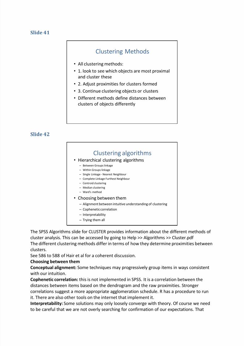
Clustering Methods
• All clustering methods:
• 1. look to see which objects are most proximal
and cluster these
• 2. Adjust proximities for clusters formed
• 3. Continue clustering objects or clusters
• Different methods define distances between
clusters of objects differently
Slide 42
Clustering algorithms• Hierarchical clustering algorithms
– Between Groups linkage
– Within Groups linkage
– Single Linkage - Nearest Neighbour
– Complete Linkage Furthest Neighbour
– Centroid clustering
– Median clustering
– Ward’s method
• Choosing between them
– Alignment between intuitive understanding of clustering
– Cophenetic correlation
– Interpretability
– Trying them all
The SPSS Algorithms slide for CLUSTER provides information about the different methods of
cluster analysis. This can be accessed by going to Help >> Algorithms >> Cluster.pdf
The different clustering methods differ in terms of how they determine proximities betweenclusters.
See 586 to 588 of Hair et al for a coherent discussion.
Choosing between them
Conceptual alignment: Some techniques may progressively group items in ways consistent
with our intuition.
Cophenetic correlation: this is not implemented in SPSS. It is a correlation between the
distances between items based on the dendrogram and the raw proximities. Stronger
correlations suggest a more appropriate agglomeration schedule. R has a procedure to run
it. There are also other tools on the internet that implement it.
Interpretability: Some solutions may only loosely converge with theory. Of course we needto be careful that we are not overly searching for confirmation of our expectations. That

8/14/2019 03 Cluster and Factor Analysis
http://slidepdf.com/reader/full/03-cluster-and-factor-analysis 30/39
said, solutions that make little sense relative to our theory, are often not focusing on the
right elements of the grouping structure.
Trying them all: It can be useful to see how robust any given structure is to a method. A
good golden rule in statistics when faced with options is: if you try all the options, and it
doesn’t make a difference which you choose in terms of substantive conclusions, then you
can feel confident in your substantive conclusions.
Slide 43
Example Clustering Using Single Linkage
Proximity Matrix
0 1533 2044 3143 1204 3042 728 2725 1427
1533 0 3100 2500 2680 1489 2270 3630 2850
2044 3100 0 1718 1268 3415 1669 4384 1010
3143 2500 1718 0 2922 3100 3387 5954 2730
1204 2680 1268 2922 0 3917 647 3911 288
3042 1489 3415 3100 3917 0 4045 4250 3991
728 2270 1669 3387 647 4045 0 3430 963
2725 3630 4384 5954 3911 4250 3430 0 4110
1427 2850 1010 2730 288 3991 963 4110 0
Case Adelaide
Alice_Springs
Brisbane
Cairns
Canberra
Darwin
Melbourne
Perth
Sydney
Adelaide Alice_Springs Brisbane Cairns Canberra Darwin Melbourne Perth Sydney
Matrix File Input
Initial Proximity Matrix
Proximity Matrix after Stage 1 Clustering
Note thenewproximitiesof theCanberra &SydneyCluster
The above hopefully illustrates the initial steps in a hierarchical cluster analysis. In the first
step, the proximity matrix is examined and the objects that make up the smallest proximity
(i.e., Sydney & Canberra – 288km) are clustered. The proximity matrix is then updated todefine proximities between the newly created cluster and all other objects. The method for
determining proximities between newly created clusters and other objects is based on the
clustering method. The above approach was based on single linkage (i.e., nearest
neighbour). In this situation the distance between the newly created cluster (C & S) with
other cities is the smaller of the distance between the other city and Canberra and Sydney.
For example, Canberra is closer to Melbourne (647km) than Sydney is to Melbourne
(963km). Thus, the distance between the new cluster (C&S) with Melbourne is the smaller of
the two distances (647km).

8/14/2019 03 Cluster and Factor Analysis
http://slidepdf.com/reader/full/03-cluster-and-factor-analysis 31/39
Slide 44
Agglomeration Schedule
5 9 288.000 0 0 2
5 7 647.000 1 0 3
1 5 728.000 0 2 41 3 1010.000 3 0 6
2 6 1489.000 0 0 6
1 2 1533.000 4 5 7
1 4 1718.000 6 0 8
1 8 2725.000 7 0 0
Stage1
2
34
5
6
7
8
Cluster 1 Cluster 2
Cluster Combined
Coeff ic ients Cluster 1 C luster 2
Stage Cluster First Appears
Next Stage
Agglomeration
Schedule
•Each row shows the
objects or clusters
being clustered
•Coefficient reflects
distance between
two objects or
clusters being
clustered
•Each object is
represented by a
number and each
cluster is represented
by the object with
the smaller number
The agglomeration schedule is a useful way of learning about how the hierarchical cluster
analysis is progressively clustering objects and clusters.
In the present example we see that in Stage 1, object 5 (Canberra) and object 9 (Sydney)
were clustered. The distance between the two cities was 288km.
In the next stage object 5 (Canberra & Sydney) and object 7 (Melbourne) were clustered.
Note that the number 5 was used to represent both Canberra (5) and Sydney (9). Why was
the distance between the combined Canberra & Sydney with Melbourne, 647km? This was
due to the use of single linkage (nearest neighbour) as the clustering method. Canberra is
closer to Melbourne than Sydney. Thus, using the nearest neighbour clustering procedure,
this distance between Canberra and Melbourne defined the distance between
Canberra/Sydney Cluster and Melbourne.
Slide 45
• Rules of interpretation
– Vertical lines indicate grouping of cases
– Cases that group earlier tend to be more similar
– Cases that group very late (e.g., Perth) are sometimes called outliers
– Drawing a vertical line through the dendrogram sets out which cases cluster
together at a given point
Dendrogram
Blue line: Potential Cluster Selection Point
A dendrogram is summarises the hierarchical agglomeration process.
Objects that group together earlier tend to be more similar in terms

8/14/2019 03 Cluster and Factor Analysis
http://slidepdf.com/reader/full/03-cluster-and-factor-analysis 32/39
of the proximity measure defined. By drawing a line through the
dendrogram we can determine which objects belong to which cluster.
The further to the right of the dendrogram we draw the line, the
fewer clusters we will extract.
Cluster 1: Canberra, Sydney, Adelaide, Melbourne, & Brisbane
Cluster 2: Cairns
Cluster 3: Alice Springs, & Darwin
Cluster 4: Perth
Slide 46
How many clusters?• Theory & Practical utility
• Sharp jump in distance between clusters
• Criteria
– AIC & BIC – See 2-step procedure
How many clusters should we extract?
Theory may provide guidance in suggesting an appropriate numbers.
Practical utility may suggest a range of values. This might range between 2 and 8 clusters. If
you imagine you are in a marketing segmentation context, it may be important that each
segment is of a sufficient size to target marketing interventions at the segment in a cost
effective manner. Thus, there may be limits on the practical value of more than a certain
number of segments. The range of what is practically useful would depend on the
circumstances and the purposes to which the cluster analysis classification is to be put.
Sharp jump in distance between clusters: The coefficient in the agglomeration schedule
indicates the distance between clusters that have been joined at a particular step in the
hierarchical clustering procedure. The nature of the procedure is that clusters are
progressively combined that are more and more dissimilar. Thus, there may be a certain
point where this coefficient does a particularly large jump. This may indicate that at this
step, one two many clusters have been combined and that dissimilar clusters are being
merged together. This can be a somewhat subjective criteria and often the increase in the
coefficient does not show this clear jump.
AIC & BIC: These are general criteria for model selection. The criteria define models as good
based on their capacity to explain variance in the cases. However, they also have a
preference for more parsimonious models. I.e., those with fewer predictors, or in the case of

8/14/2019 03 Cluster and Factor Analysis
http://slidepdf.com/reader/full/03-cluster-and-factor-analysis 33/39
cluster analysis, fewer clusters. The clustering solution with the smallest AIC or BIC is chosen.
This is implemented in SPSS’s newer two-step cluster analysis procedure.
Conclusion: In general I tend to rely on theory and practical utility and an overall visual
assessment of the dendrogram. It could also be argued that the very nature of hierarchical
cluster analysis is to explore the hierarchical structure of the objects. Thus, cluster solutions
maybe useful at multiple levels giving either big picture or detail depending on one’s
interests.
Slide 47
Hierarchical Cluster AnalysisDerived Distances
• Example
– Cases Faculty Members of Department of Psychology at
East Carolina University, Nov 2005
• Variables
– Annual Salary
– Full Time Equivalent Workload
– Rank (5 levels) from adjunct to professor
– Number of published articles
– Years as full time faculty member in a psychology
department
– Sex
• Research Methods
This is based on an example dataset taken from:
http://core.ecu.edu/psyc/wuenschk/SPSS/ClusterAnalysis-SPSS.docThe actual data files are located on:
http://core.ecu.edu/psyc/wuenschk/SPSS/SPSS-Data.htm
You may wish to run this analysis in SPSS. Karl L. Wuensch provides suggestions for how you
might run it.
Slide 48
Another Example - Clustering countriesCase Summariesa
Australia 31 12 80 5 .10 20 4.7
Braz il 8 17 72 12 .70 186 29.6
China 6 13 72 10 .10 1306 24.2
Croatia 11 10 74 14 .10 4 6.8
Finland 29 11 78 9 .10 5 3.6
Japan 29 9 81 5 .10 127 3.3
Mexico 10 21 75 3 .30 106 20.9
Russia 10 10 67 8 1.10 143 15.4
UnitedKingdom
30 11 78 5 .20 60 5.2
UnitedStates
40 14 78 6 .60 296 6.5
10 10 10 10 10 10 10 10
1
2
3
4
5
6
7
8
9
10
NTotal
country
GDP Per
Capita($1,000) b ir thRate
lifeExpectAtBirth
unemploymentRate hivPrevalence
Population(Million)
infantMortalityRate
Limited to first 100 cases.a.
1. How would you arrange countries in the world into clusters?
2. What variables would you use as the basis of the clustering?
3. If we use the above variables, how would you cluster the above countries?

8/14/2019 03 Cluster and Factor Analysis
http://slidepdf.com/reader/full/03-cluster-and-factor-analysis 34/39
Data extracted from 2004 CIA World Fact book using MarketStatistics {fEcofin} in R
It is useful to ask the above questions in an intuitive sense before using sophisticated
statistical software.
Clearly for different purposes, we would group countries in different ways. Depending on our
purposes, we would choose different variables from which to derive our proximities.
Slide 49
Proximity Measures
• Squared Euclidean Distance
• Raw Data (Transform Values – Z scores)
• Rescale Proximities (Transform Measures – Rescale to 0-1 range)
Proximity Matrix
.00 .85 .94 .43 .05 .01 .50 .89 .00 .13
.85 .00 .49 .51 .73 1.00 .37 .34 .78 .69
.94 .49 .00 .66 .84 .96 .72 .80 .86 .89
.43 .51 .66 .00 .18 .44 .83 .56 .38 .61
.05 .73 .84 .18 .00 .06 .66 .73 .04 .20
.01 1.00 .96 .44 .06 .00 .68 .92 .01 .19
.50 .37 .72 .83 .66 .68 .00 .79 .52 .51
.89 .34 .80 .56 .73 .92 .79 .00 .70 .65
.00 .78 .86 .38 .04 .01 .52 .70 .00 .11
.13 .69 .89 .61 .20 .19 .51 .65 .11 .00
Case
1:Australia
2:Brazil
3:China
4:Croatia
5:Finland
6:Japan
7:Mexico
8:Russia
9:UnitedKingdom
10:UnitedStates
1:A ust ral ia 2: Br azi l 3: Ch ina 4:Cr oat ia 5:Fi nl and 6:Ja pan 7: Mexic o 8: Ru ssi a9:UnitedKingdom
10:UnitedStates
Rescaled S quared Euclidean Distance
This is a dissimilarity matrix
Squared euclidean is typical of many distance based proximities. We are interested in
absolute differences in levels on the variables.
Raw data was standardised because the variables such as GDP and infant mortality were on
vastly different measurement scalesProximities were rescaled simply to make interpretation of the output above more
meaningful. Values closer to zero indicate greater similarity. Values closer to one indicate
greater dissimilarity.
Looking at the proximity measure, we see that Australia, United Kingdom and Japan are very
similar.
Slide 50
Dendrogram
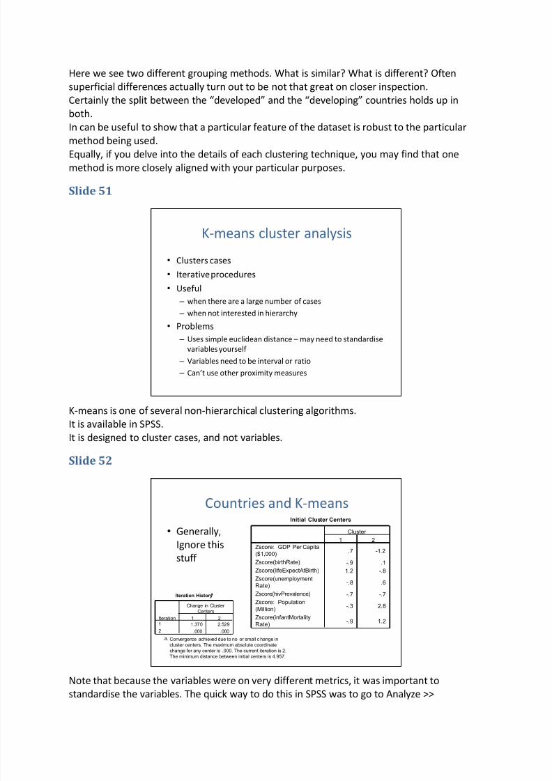
8/14/2019 03 Cluster and Factor Analysis
http://slidepdf.com/reader/full/03-cluster-and-factor-analysis 35/39
Here we see two different grouping methods. What is similar? What is different? Often
superficial differences actually turn out to be not that great on closer inspection.
Certainly the split between the “developed” and the “developing” countries holds up in
both.
In can be useful to show that a particular feature of the dataset is robust to the particular
method being used.
Equally, if you delve into the details of each clustering technique, you may find that one
method is more closely aligned with your particular purposes.
Slide 51
K-means cluster analysis
• Clusters cases
• Iterative procedures• Useful
– when there are a large number of cases
– when not interested in hierarchy
• Problems
– Uses simple euclidean distance – may need to standardise
variables yourself
– Variables need to be interval or ratio
– Can’t use other proximity measures
K-means is one of several non-hierarchical clustering algorithms.It is available in SPSS.
It is designed to cluster cases, and not variables.
Slide 52
Countries and K-means
• Generally,
Ignore thisstuff
Iteration Historya
1.370 2.529
.000 .000
Iteration1
2
1 2
Change in Cluster Centers
Convergence achieved due to no or small c hange incluster centers. The maximum absolute coordinatechange for any center is .000. The current iteration is 2.The minimum distance between initial centers is 4.957.
a.
Initial Cluster Centers
.7 -1.2
-.9 .1
1.2 -.8
-.8 .6
-.7 -.7
-.3 2.8
-.9 1.2
Zscore: GDP Per Capita($1,000)
Zscore(birthRate)
Zscore(lifeExpectAtBirth)
Zscore(unemploymentRate)
Zscore(hivPrevalence)
Zscore: Population(Million)
Zscore(infantMortalityRate)
1 2
Cluster
Note that because the variables were on very different metrics, it was important tostandardise the variables. The quick way to do this in SPSS was to go to Analyze >>

8/14/2019 03 Cluster and Factor Analysis
http://slidepdf.com/reader/full/03-cluster-and-factor-analysis 36/39
Descriptives >> Descriptive Statistics, place the variables in the list and select “Save as
Standardized variables”. I then use these new variables in the k-means analysis. For the
curious when I did not do this, China came out all on its own, probably because population
as it is coded has the greatest variance and it was very different to all the other countries.
The above tables highlight the iterative nature of k-means cluster analysis. I chose two
clusters, but it would be worth exploring a few different numbers perhaps from 2 to 4.
Do not interpret the initial cluster centers. It is merely an initial starting configuration for the
procedure. The countries were then shuffled between groups iteratively until the variance
explained by the grouping structure was maximised. In this case this was achieved in only 2
iterations. In more complex examples, it may take many more iterations.
Slide 53
Cluster MembershipCluster Membership
Australia 1 .932
Braz il 2 1.602
China 2 2.529
Croatia 1 2.673
Finland 1 1.063
Japan 1 1.370
Mexico 1 3.187
Russia 2 2.263
UnitedKingdom
1 .804
UnitedStates
1 1.770
Case Number 1
2
3
4
5
6
7
8
9
10
country Clus ter Dist ance
Final Cluster Cen ters
.4 -1.0
-.1 .1
.5 -1.2
-.3 .7
-.4 .8
-.4 .8
-.5 1.1
Zscore: GDP Per Capita($1,000)
Zscore(birthRate)
Zscore(lifeExpectAtBirth)
Zscore(unemploymentRate)
Zscore(hivPrevalence)
Zscore: Population(Million)
Zscore(infantMortalityRate)
1 2
Cluster
Number of Cases in ea ch Cluster
7.000
3.000
10.000
.000
1
2
Cluster
Valid
Missing
istances between Final Cluster Centers
3.378
3.378
Cluster 1
2
1 2
This output shows the cluster membership of each of the countries. Larger Distance values
indicate that the case is less well represented by the cluster it is a member of. For example,
Mexico, although assigned to cluster 1, is less well represented by the typical profile of
cluster 1. We see that it has grouped China, Brazil, and Russia together.
We can also look at the Final Cluster Centers and interpret what is typical for a particular
cluster. In this case the variables are z-scores, cluster 2 is characterised by lower than
average GDP per capita and life expectancy and higher than average unemployment HIV
prevalence, population and infant mortality.
Distances between Final Cluster Centers indicates the similarity between clusters. It is ofgreater relevance when there is multiple clusters and the relative size of the distance gives
some indication regarding which clusters are relatively more or less distinct.
You can perhaps imagine how such an interpretation would operate in a market
segmentation context. You might be describing your sample in terms demographic or
purchasing behaviour profiles. Assuming you have a representative sample, you might also
be able to describe the relative size of each segment.

8/14/2019 03 Cluster and Factor Analysis
http://slidepdf.com/reader/full/03-cluster-and-factor-analysis 37/39
Slide 54
Choosing between cluster analytic
techniques• Hierarchical cluster analysis
– Problematic with large number of cases
– Useful for analysing variables and other types of objects
– Useful for exploring hierarchical structures when they are
present
• K-means
– Useful when there are a large number of cases
– Typically produces fairly even sized homogenous groups
– Fewer options to get lost in regarding agglomeration
– Remember to assess need for variable standardisation
• Also see two-step and many more
Slide 55
Multidimensional Scaling
• Another tool for modelling associations between objects
• Particular benefits
– Spatial representation
• Complimentary to cluster analysis and factor analysis
– Measures of fit
• Example
– Spatial representation of ability tests
• References
– See Chapter 9 MDS of Hair et al
– http://www.statsoft.com/textbook/stmulsca.html

8/14/2019 03 Cluster and Factor Analysis
http://slidepdf.com/reader/full/03-cluster-and-factor-analysis 38/39
Slide 56
Cluster Analysis & Factor AnalysisCommon Purposes
• Grouping objects
• Determining how many groups are needed
• Relationships between groups
• Outliers
• Other forms of structure
GROUPING OBJECTS: Objects can be cases or variables. Objects can be survey items,
customers, products, countries, cities, or any number of other things. One aim of the
techniques presented today is to work out ways of putting them into groups.
DETERMINING HOW MANY GROUPS ARE NEEDED: In factor analysis, it was the question of
how many factors are needed to explain the variability in a set of items. In Cluster analysis,
we looked at how many clusters were appropriate.
RELATIONSHIP BETWEEN GROUPS: In factor analysis we get the component correlation
matrix which shows how the correlation between the extracted factors. In hierarchical
cluster analysis we can see how soon two broad clusters merge together. In k-means cluster
analysis we have the measure of distance between clusters.
OUTLIERS: Factor analysis has variables with low communalities, low factor loadings and low
correlations with other items. Hierarchical cluster analysis has objects that to do not group
with other variables until a late stage in the agglomeration schedule. K-means can have
clusters with only a small number of groups.
Other forms of structure: Factor analysis is specifically designed for pulling out latent factors
that are assumed to have given rise to observed correlations. Hierarchical cluster analysis
can reveal hierarchical structure.

8/14/2019 03 Cluster and Factor Analysis
http://slidepdf.com/reader/full/03-cluster-and-factor-analysis 39/39
Slide 57
Core Themes
• Reasoned decision making
– Recognise options >> evaluate options >> justify decision
• Simplifying structure
• Answering a research Question
• Tools for building subsequent analyses
Reasoned decision making: There are many options in both factor analysis and cluster
analysis. It is important to recognise that these options exist. Determine what the arguments
are for against different options. Often the best option will depend on what your theory is
and what is occurring in your data. Once it is time to write it up, incorporate this reasoning
process into your write-up. You may find it useful to cite statistical textbooks or the primary
statistical literature. Equally you might proceed from first principle in terms of the underlying
mathematics. Your writing will be a lot stronger and defensible if you have justified your
decisions.