027-042 ijmr 110250 27. - Case School of Engineering

Rick Rajtera, Roger H. FrenchbaMassachusetts Institute of Technology, Cambridge, MassachusettsbDuPont Co. Central Research, Wilmington, Delaware

Van der Waals–London dispersion interactionframework for experimentally realistic carbonnanotube systems

A system’s van der Waals–London dispersion interactionsare often ignored, poorly understood, or crudely approxi-mated, despite their importance in determining the intrinsicproperties and intermolecular forces present in a given sys-tem. There are several key barriers that contribute to this is-sue: 1) lack of the required full spectral optical properties,2) lack of the proper geometrical formulation to give mean-ingful results, and 3) a perception that a full van der Waals–London dispersion calculation is somehow unwieldy or dif-ficult to understand conceptually. However, the physicalorigin of the fundamental interactions for carbon nanotubesystems can now be readily understood due to recent devel-opments which have filled in the missing pieces and pro-vided a complete conceptual framework. Specifically, ourunderstanding is enhanced through a combination of a ro-bust, ab-initio method to obtain optically anisotropic prop-erties out to 30 electron Volts, proper extensions to the Lif-shitz’s formulations to include optical anisotropy withincreasingly complex geometries, and a proper methodol-ogy for employing optical mixing rules to address multi-body and multi-component structures. Here we review thisnew framework to help end-users understand these interac-tions, with the goal of better system design and experimen-tal prediction. Numerous examples are provided to showthe impact of a material’s intrinsic geometry, including op-tical anisotropy as a function of that geometry, and the ef-fect of the size of the nanotube core and surfactant materialpresent on its surface. We’ll also introduce some new ex-amples of how known trends in optical properties as a func-tion of [n, m] can result in van der Waals interactions as afunction of nanotube classification, radius, and other pa-rameters. The concepts and framework presented are notlimited to the nanotube community, and can be equally ap-plied to other nanoscale or even biological systems.

Keywords: Carbon nanotubes; van der Waals

1. Introduction

Van der Waals–London dispersion (vdW–Ld) interactionsarising from quantum electrodynamics (QED) are of consid-erable importance to scientists and engineers across manydisciplines. First, they are influential in behaviors rangingfrom colloidal interactions in solution to the fracture behav-

ior of bulk materials [1]. Second, the vdW–Ld interactionsare even influential when so-called “stronger” forces, suchas electrostatic or polar interactions, are present [2]. And fi-nally, they are universally long range interactions that canonly be nullified by carefully designing the system to balancethe attractive and repulsive components of the overall inter-action [3]. Thus the study of van der Waals–London disper-sion spectra (vdW–LDS) and forces can enrich our under-standing of particular phenomena, which is important forscientists and engineers interested in using self-assemblyprocesses to create nanoscale structures and devices.

But despite being important and of interdisciplinary in-terest, vdW–Ld interactions calculated from a first princi-ples, QED approach (i. e., the Lifshitz formulation [4]) havea reputation for being intractable or difficult to use and un-derstand. Thus it is very common to use outdated pairwisemodels with Lennard–Jones potentials, ignoring the funda-mental electrodynamics and the important many-body ef-fects. Admittedly, there are two barriers that can still pre-vent people from getting started:1. the lack of the full spectral optical properties of all the

components within the system, and2. the lack of an analytically tractable solution for the sys-

tem geometry of interest. While both of these are still is-sues today, much progress has been made on both frontsin the past 20 years [1–3, 5].

First, the formulations have been extended to includeeverything from an infinite number of layers (stacked inthe semi-infinite half-space formulation), to optically an-isotropic solid cylinders interacting with each other in saltsolutions [6]. Recently the formulations for solid cylinderswere extended even further in order to incorporate opticalanisotropy into the solid cylinder–cylinder and cylinder–substrate formulations at the near and far-limits. The abilityto combine all these new features is essential for metallicsingle-wall carbon nanotubes (SWCNTs) due to the largedegree of optical anisotropy coupled with their large mor-phological aspect ratios [7]. And we are by no means lim-ited to just rods and flat planes. A recent book publishedby Parsegian also contains a large array of vdW–Ld formu-lations for different geometries [3].

Second, the advent of robust, fast, and reliable ab-initiocodes has allowed for the calculation of full spectral opticalproperties for materials which are either very difficult orimpossible to quantitatively measure experimentally. Ex-perimental methods like vacuum ultraviolet (VUV) reflec-

R. Rajter, R. H. French: Van der Waals–London dispersion interaction framework

Int. J. Mat. Res. (formerly Z. Metallkd.) 101 (2010) 1 27

BBasicW

2010

Car

lHan

ser

Ver

lag,

Mun

ich,

Ger

man

yw

ww

.ijm

r.de

Not

for

use

inin

tern

etor

intr

anet

site

s.N

otfo

rel

ectr

onic

dist

ribut

ion.

tivity for bulk optical properties [8], transmission valenceelectron energy loss spectroscopy (VEELS) for interfacialoptical properties [8], or reflection VEELS for surfaces [9]are still useful for the characterization of many materials.But for nanoscale materials like SWCNTs, techniques likeEELS result in many inherent inaccuracies in the anisotro-pic spectral optical properties because of the difficulty inisolating, aligning, measuring and then analyzing the mea-sured signals off a single SWCNT. Thus ab-initio computa-tions of full spectral optical properties eliminate this barrierby offering a way to obtain this data for nanoscale materialswith results that are directly comparable.

With the introduction of ab-initio optical properties andLifshitz formulations designed for SWCNTs, it is now pos-sible to begin calculating vdW–Ld interactions for a limitednumber of systems (i. e., systems containing SWCNTs onlywith no surfactant). However, a crucial piece is still neededto address all potential system variations relevant for ex-perimentalists (e. g., surfactant coated SWCNTs, multi-wallCNTs, and SWCNTs having a very large core volume [17]).For planar systems, this issue was alleviated by the intro-duction of the “add-a-layer” approach [1] in which the3-component solution was expanded to include an infinitenumber of parallel layers of arbitrary ordering and thick-ness. The boundary conditions of parallel planes made thisa straightforward process after the initial expansion wasgenerated [3]. Unfortunately, the cylindrical geometrieshave no equivalent analytical form to include such layerstacking as a function of cylinder radius. And without theability to address this radial spatial variation, the effects of

ssDNA (single-stranded DNA), SDS (sodium dodecyl sul-fate), and other well known surfactants would have to beignored.

Fortunately there is a viable alternative to an add-a-layerformulation. Spectral mixing to produce effective mediumspectra [10] for use at the appropriate surface-to-surface se-paration limits can be used to create effective vdW–LDSthat results in an exact total vdW–Ld energy. In principle,this is no different than if we took a highly spatially re-solved optical spectra of water (clearly oxygen and hydro-gen locations have different quantities of electrons andwave functions) and averaged it back to the isotropic valuethat has been thoroughly studied and used for decades [3,11–14].

With the ab-initio optical properties [15], optically aniso-tropic cylinder formulations [7, 16], and mixing formula-tions for SWCNT systems now in place [17], a full frame-work for calculation of the vdW–Ld interactions forSWCNTs is now available. This is summarized in the flowchart found in Fig. 1. To see the actual optical spectra andvdW–Ld properties as they relate to SWCNTs through thesteps in the flow chart, see Figs. 2 and 3, which track theseproperties from the chirality indices [n, m] to the angulardependent Hamaker coefficients (the material componentof the total vdW–Ld energy) for the [6,5,s] semiconductingand [9,3,m] metal SWCNTs. The vdW–Ld framework pre-sented here is being implemented in Gecko Hamaker, a freeand open source software package which contains opticalproperties and various geometrical formulations appropri-ate to vdW–Ld interaction science [19].


28 Int. J. Mat. Res. (formerly Z. Metallkd.) 101 (2010) 1

BBasic

Fig. 1. The complete flow chart of the Lifshitzformulation/framework that is necessary forcalculating and understanding the physical ori-gin of the chirality-dependent Hamaker coeffi-cients and vdW–Ld total energies of SWCNTsystems.

W20

10C

arlH

anse

rV

erla

g,M

unic

h,G

erm

any

ww

w.ij

mr.

deN

otfo

rus

ein

inte

rnet

orin

tran

etsi

tes.

Not

for

elec

tron

icdi

strib

utio

n.

What follows is an end-user tutorial highlighting key fea-tures within Fig. 1 as they relate to Figs. 2 and 3. Althoughdetermining vdW–Ld interactions for SWCNT systemstends to be more complicated than isotropic plane–planesystems, the overall form of the Lifshitz calculation re-mains common across many types of geometries of increas-ing complexity. Numerous examples are included to de-monstrate the major effects of varying optical properties,Lifshitz geometry, and mixing rules in order to guide thereader. Finally, we include some emerging results fromour upcoming data-mining analysis across 63 SWCNTs.The optical properties as a function of radius and metallic/semiconducting classification trend in both obvious andsurprising ways when carried through to the final Hamakercoefficients and total energies.

2. Background

2.1. vdW–Ld Theory

A brief overview of the link from optical properties [20] toHamaker coefficients is useful before comparing and con-trasting the different vdW–Ld formulations [3]. The keysource of all vdW–Ld interactions is optical contrast be-tween each system interface. The index of refraction (an op-tical property) serves as a useful proxy for the dispersion orpolarizability in this discussion, while the vdW–Ld interac-tion is based more accurately on another optical property,the London dispersion spectra, across a wider range of fre-quencies. If there were no optical contrast in the universe,

then all materials would be equally polarizable and all elec-tromagnetic radiation would move from phase to phase,passing through a variety of interfaces or boundaries thesame way. Without optical contrast, there would be no pre-ferential placement of particular objects and hence novdW–Ld interaction to lower the system’s free energy. Butoptical contrast does exist among different materials andover a wide range of optical frequencies. It is this contrastthat opens the door for attractive and repulsive vdW–Ld in-teractions depending upon the many possible componentsin a system.

2.1.1. Buoyancy illustration

A buoyancy illustration can be quite helpful in understandingthe many-body vdW–Ld interaction at its most primitive lev-el. In Fig. 4, we note that the two different blocks of materialsrest on the ground in air. If we were to try and separate theseblocks along the vertical axis, gravity would pull the blocksback down towards one another. This is similar to any twomaterials in vacuum. They are each more polarizable in airthan when compared to the vacuum, and thus “fall” towardseach other in order to minimize the system’s energy.

The many-body nature of the interaction becomes appar-ent when we add water (the medium) to a system with oneblock of a higher density and one of a lower density than



BBasic

Fig. 2. Part 1 of the chirality-dependent vdW–Ld interaction analysisfor the [6,5,s] and [9,3,m]. (a) The [n, m] vector placed upon the gra-phene sheet denotes the circumference of the SWCNT. (b) TheSWCNTs x, y, z positions in space. Note the structural difference inthe twisting. (c) The cutting lines within the Brillouin zone, varying inquantity and angle based on the specific [n, m] magnitudes and magni-tude ratio between them. (d) The band diagrams determined by the al-lowable states along the cutting lines. Stages E through G are continuedin Fig. 3.

Fig. 3. Part 2 of the chirality-dependent vdW–Ld interaction analysisfor the [6,5,s] and [9,3,m]. (e) The allowable single electron transitionsdetermine the optical absorption part of the dielectric spectrum, e00ðxÞ,over all real frequencies. (f) The vdW–LDS obtained via the KK trans-form upon e00ðxÞ. Note the differences between a SWCNTs radial andaxial directions as well as the differences between the tubes. (g) Ha-maker coefficients in a solid cylinder SWCNT–water–gold substratesystem as a function of ‘. Additional and/or later stages include an ana-lysis of DOS/JDOS as well as total vdW–Ld energies.

W20

10C

arlH

anse

rV

erla

g,M

unic

h,G

erm

any

ww

w.ij

mr.

deN

otfo

rus

ein

inte

rnet

orin

tran

etsi

tes.

Not

for

elec

tron

icdi

strib

utio

n.

the water (Fig. 4 part C). In this situation, there is a “repul-sive” force between the two blocks as a result of one sink-ing and one floating in the liquid medium. Other blocksadded would rise or sink depending on their own respectivebuoyancies. A similar effect occurs with the vdW–Ld inter-actions. If the medium’s optical properties (e.g., index ofrefraction) is intermediate to that of the two objects, the sys-tem will minimize its overall energy by moving those twoobjects far apart. But if both materials either have lower orhigher indices of refraction than the water medium, theywill attract towards each other again. This is equivalent tothe interacting blocks both being more or less dense thanthe water and driving towards one another. In either case,attraction between A and B only occurs if the medium iseither more or less dense than each object present.

We could extend the buoyancy analogy further to describemore complicated phenomena. For instance, we couldchange the medium’s density by adding an additional com-ponent or changing the temperature. An example of this is aGalileo thermometer [21], where changes in temperature cre-ate a change in the ambient liquid density. The temperatureindicators (of a relatively fixed density versus temperature)then begin to rise/fall as this change occurs. Another exten-sion of the buoyancy analogy is that of a multi-componentsystem, such as a boat. While the outer shell of an oil tankeris far more dense than the water, the total density over the en-tire ship is such that the boat floats. The effect is similar forvdW–Ld forces, where the magnitude and percent volumeof the components present dictate the overall attraction toplanes of higher and lower optical density.

There are, however, a few areas where the buoyancy il-lustration and a vdW–Ld interaction are not truly analo-gous. The first is that vdW–Ld interactions arise from opti-cal contrast across ALL optical frequencies as opposed tobuoyancy’s reliance on a single term (weight density).What this means is that a vdW–Ld interaction between ob-jects in a system can have both attractive and repulsiveparts for a given medium and materials A and B. Yet the in-teraction at a given frequency is still identical to a snapshotof relative buoyancy. It is therefore essential to consider all

the frequencies in the electrodynamic interaction, not tooversimplify to one or a few interaction frequencies. Thisis due to the fact that the entire frequency range contributesto the overall Lifshitz summation, with a bulk of this contri-bution coming from frequencies of higher energy than visi-ble light.

The analogy is also not consistent when considering thebehavior of the system as the medium’s thickness or the se-paration distance changes. Buoyancy does not show many-body effects which vary as a function of separation dis-tances. But the vdW–Ld interaction has a fundamental scal-ing of the separation distance and the optical penetrationdepth (sampling depth), or the interaction volume of thetwo bodies which determines what parts of the two bodiesare dominating the interaction at a given separation. For ex-ample in the near limit, where the separation of the twobodies is much smaller than their size, then the surface ofthe two bodies is controlling, while at long separation dis-tances the average properties of the whole bodies is impor-tant. This is mainly a result of the inverse power-law scal-ing of the total vdW–Ld interaction energy. Understandinghow the different components of each body contribute as afunction of the surface-to-surface separation is an importantdeparture from the buoyancy analogy, which is equivalentto the far-limit.

Despite its shortcomings, the buoyancy illustration is aconceptually easy to understand model that can be usefulin understanding the quantitative and qualitative impactof each component within the full Lifshitz framework(Fig. 1). Upon a closer analysis of these interdependencies,one can have a better understanding of the fundamentalworkings of the interactions and thereby make smarter deci-sions on experimental design.

3. The fundamental framework

3.1. Ab-initio optical properties

If the source of a van der Waals interaction is optical con-trast at all system interfaces, then it is imperative to obtainthe optical spectra for all the components present in thesystem to the highest accuracy possible. This typicallyrequires having the imaginary part of the dielectric func-tion (e00 spectra) for each material over an interval from0–30 electron volts (eV) to ensure complete convergence.The way that the particular optical properties are obtainedis only relevant if there are particular caveats to consider,such as a particular frequency/energy range where the datatend to not be certain. Beyond that, the various experimen-tal or ab-initio optical properties are interchangeable. Forexample: some choose to view the results in Jcv(eV) form(interband transition strength) while others prefer dielec-tric function over real frequencies (e00(x)). The choicereally depends upon the optical property features that areunder investigation because Jcv(eV) and e00(x) weight thepeaks differently. One can convert between the two viathe following:

JcvðeVÞ ¼m2

o

e2�h2eV2

8p2ðe00ðeVÞ þ {e0ðeVÞÞ ð1Þ

Where Jcv(eV) is proportional to the interband transitionprobability and has units of g � cm�3. For computational



BBasic

Fig. 4. An illustration relating the similar effects of optical contrast ina far-limit vdW–Ld interaction with that of density contrast (i. e. rela-tive buoyancy). It is the relative contrast between all components thatdetermines whether there is a net attraction or repulsion between any2 given components in the overall system. Material density is indicatedby color with white being vacuum and black or very dark colors beingthe most dense.

W20

10C

arlH

anse

rV

erla

g,M

unic

h,G

erm

any

ww

w.ij

mr.

deN

otfo

rus

ein

inte

rnet

orin

tran

etsi

tes.

Not

for

elec

tron

icdi

strib

utio

n.

convenience, we take the prefactor m2oe

�2�h�2 in Eq. (1),whose value in cgs units is 8:29 � 10�6 g � cm�3 � eV�2, asunity [1]. For vdW–Ld calculations, the optical data needsto be converted into vdW–LDS. Assuming e00 is properlyscaled to the correct magnitude, this is done using the fol-lowing form of the Kramers–Kronig (KK) transformation:[3, 15, 20].

eð{nÞ ¼ 1þ 2p

Z 1

0

e00ðxÞ � xx2 þ n2

dx ð2Þ

We refer to eð{nÞ, a real function over the imaginary fre-quency domain, as the vdW–Ld spectrum (or vdW–LDS)in order to differentiate it from the dielectric function overreal frequencies ðe00ðxÞÞ. Although the eð{nÞ form of the op-tical spectra appear to be simple damped oscillators, theycontain the complete electronic structure and interatomicbonding of the materials, i. e., the interband transitions thatdetermine the optical properties. Additionally, small differ-ences in both the magnitude and stacking order of the vdW–LDS in a geometrical configuration can influence both themagnitude and the sign of the total vdW–Ld interaction en-ergy. For our SWCNT calculations, we use the e00 proper-ties, obtained from ab-initio orthogonal linear combinationof atomic orbital (OLCAO) computations [22–27], thathave been scaled to the solid and hollow cylinder geome-tries [17].

One final issue should be addressed before moving on.Some researchers may have concerns over the usage ofab-initio optical properties for fear that they may be inac-curate or unrealistic in comparison to experimental data.A typically cited concern is the discrepancy that exists be-tween experiment and theory in band gap calculations,particularly for models that employ simplifications likethe tight binding approximation. However, vdW–Ld inter-actions are dependent upon all the electronic transitions,with significant transitions occurring in the deep UVranges up to 30 eV and higher. The full OLCAO calcula-tion captures this correctly because it contains completeorbital information up to the 4p and 3d shells. The resultshave compared very well to experimental e00 data and Ha-maker coefficient calculations for systems like graphite,ZrO2, AlN, LiB2O3 and including organic materials withhydrogen such as polysilane [23–27]. This gives us confi-dence in using this data for systems like SWCNTs, whichwe believe to be very difficult to accurately obtain experi-mentally because of the small size and cylindrical shape ofthese materials. By using an ab-initio method, we can eas-ily and systematically calculate the optical properties forall possible SWCNT types.

As for the actual method, the primary equation for ob-taining e00ðxÞ from the band structure is as follows [22–26]:

e00ijðxÞ ¼4p2e2

Xm2x2

Xknn0r

hknrjpijkn0rihkn0rjpjjknrifknð1� fkn0 Þ

dðekn0 � ekn � �hxÞ ð3Þ

Here again e00ðxÞ is the imaginary part of the dielectricspectrum at a given frequency x, with mass m, and Bril-louin zone volume X. The momentum operators, pi and pj,operate on both the valence and conduction band wavefunctions, where the i and j subscripts represent the direc-tions of the tensor in three dimensional space. The Fermifunction (fkn) terms ensure that only transitions between anoccupied valence to an unoccupied conduction band transi-tion are allowed, and the delta function ensures that onlytransitions corresponding to the particular energy �hx areconsidered.

This is simply the ab-initio way of obtaining the data.There are also various experimental results which provideexcellent corroboration. As an example, Stephan et al. havedone impressive work obtaining experimental e00 data forSWCNTs along the axial direction by applying a grazingangle EELS measurement [28]. Despite some noise in thedata and the lack of chirality/direction identification, the e00

results corroborate many of the key features (most notablythe large e00 peaks around 15 eV) of the present authors’ab-initio data. New results published just last year add sup-port for these peak positions and magnitudes [29]. The en-ergy loss function determined from EELS data, though use-ful for qualitative corroboration, cannot itself be used forthe calculation of certain properties (e. g., a vdW–Ld inter-action) because it is arbitrarily scaled along its y-axis andthus lacks the necessary quantification. But having boththe experimental and ab-initio properties gives us quantita-tive data that we can confidently use because of their agree-ment. These fundamental optical properties can then beused for predictive experimental design schemes for sys-tems using dielectrophoresis (DEP) or having sensitivevdW–Ld interactions.

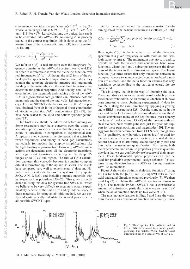
Figure 5 shows the ab-initio dielectric function e00 usingEq. (3) for both the [6,5,s] and [9,3,m] SWCNTs in theiraxial and radial directions obtained previously [7]. We thenused Eq. (2) to obtain the vdW–Ld spectra as shown inFig. 6. The metallic [9,3,m] SWCNT has a considerableamount of anisotropy, particularly at energies near 0 eVwhen the axial direction shoots up to a value of 333.

The most notable features in Figs. 5 and 6 are the varia-tions that exist as a function of direction and chirality. Since



BBasic

Fig. 5. The e00 spectra of the (a) [6,5,s] and (b)[9,3,m] SWCNTs scaled to a solid cylindergeometry. The metallic [9,3,m] SWCNT axialdirection spikes to a value of 930 at 0.04 eV.

W20

10C

arlH

anse

rV

erla

g,M

unic

h,G

erm

any

ww

w.ij

mr.

deN

otfo

rus

ein

inte

rnet

orin

tran

etsi

tes.

Not

for

elec

tron

icdi

strib

utio

n.

the vdW–LDS are the very inputs to the full Lifshitz formu-lation, one can observe a clear possibility for a chirality-de-pendent vdW–Ld interaction. Of course, the magnitude ofsuch an interaction needs to be determined.

3.2. Lifshitz formulations

Once we have the vdW–Ld spectra for the materials within agiven system, the Lifshitz formulation weights their opticalcontrast contributions at the required Matsubara frequenciesand determines the vdW–Ld interaction strength by a singleHamaker coefficient A. The Hamaker coefficient (which isapproximately the volume–volume vdW–Ld interactiondensity or strength between two components of a system)is then multiplied by the proper geometrical scale factor todetermine the vdW–Ld interaction energy or force. Thusthe general form of the vdW–Ld energy is [3, 15]:

G ¼ �A � g‘n

ð4Þ

where G is the thermodynamic free energy, g is a collectionof geometry factors (e. g. g ¼ pa2=6 per unit of cylinderlength for the far-limit, cylinder–substrate geometry wherea is the nanotube radius), and ‘n is the scaling law behaviorat a surface-to-surface separation distance ‘ for a given geo-metry. EssentiallyA is the interaction strength as a functionof the material properties of two objects within the givengeometry, whereas g and n depend solely by the systemgeometry itself. Geometry affects the magnitude of the Ha-maker coefficient because the optical contrast functionschange as a function of geometry in the Lifshitz summation,and cannot be decoupled into a strictly material-dependentexplanation. To demonstrate this coupling further, we shallobserve the change of the optical contrast functions as afunction of increasing geometrical complexity, rangingfrom the simple isotropic plane–plane geometry to the cy-linder–cylinder interactions relevant for SWCNT systems.

The calculation of A for the non-retarded case1 over allthree levels of complexity has a consistent general form:

ANR ¼ 3kbT2

� 12p

X1n¼0

0 Z 2p

0DLmDRmdu ð5Þ

where n denotes the discrete Matsubara frequencies

(nn ¼2pkbT

�hn) ranging from 0 to 1, the values DLm and

DRm are the spectra mismatch functions comparing thevdW–Ld spectra properties of the particular material L orR with the neighboring medium m. The prime on the sum-mation denotes that the first frequency n ¼ 0 is multipliedby 0.5.

It is with this general form that we can compare all threesystems (Fig. 7). When looking at this figure, pay specialattention to how the components of spectral mismatch func-tions (i. e. DLm and DRm) vary as a function of the geometry.Changes in the forms of these weighting functions can havea substantial impact in changing the sign and magnitude ofthe overall interaction.

3.2.1. Optically isotropic planar system

The isotropic plane–plane system (see Fig. 7a) is the mostcommonly used of all the Lifshitz formulations because itis by far the easiest to calculate and it is the most relevantfor the interactions of large bulk materials. Its energy perunit area is

G ¼ ANR

12p‘2ð6Þ

Because the left and right half-spaces are both isotropic,there is no angular dependance of the vdW–Ld interactionfor rotations about the interface normal of either half space.Therefore the integration around angle du leads to constant

value of 2p which cancels out the12p

coefficient in the gen-eral form to leave us with

A ¼ 3kbT2

X1n¼0

0

DLm � DRm ð7Þ

The DLm and DRm terms are as follows

DLmð{nnÞ ¼eLð{nnÞ � emð{nnÞeLð{nnÞ þ emð{nnÞ

ð8ÞDRmð{nnÞ ¼

eRð{nnÞ � emð{nnÞeRð{nnÞ þ emð{nnÞ

We normally drop the explicit ð{nnÞ notation for clarity asit is assumed that all vdW–Ld spectra are frequency de-pendent and only calculated at each Matsubara frequencyðnnÞ (where each n represents a change of 0.16 eV for the

case of 300 K). These mismatch terms all have ana� b

aþ bform, which can never exceed a value of 1 because the



BBasic

Fig. 6. The vdW–Ld spectra of the (a) [6,5,s]and (b) [9,3,m] SWCNTs scaled to a solid cy-linder geometry and compared to the indexmatching water spectra. The [9,3,m] axial di-rection spikes up to a value of 333 at 0 eV.

1 In the non-retardedc case, we neglect the finite speed of light travel-ing back and forth between the interacting sides.

W20

10C

arlH

anse

rV

erla

g,M

unic

h,G

erm

any

ww

w.ij

mr.

deN

otfo

rus

ein

inte

rnet

orin

tran

etsi

tes.

Not

for

elec

tron

icdi

strib

utio

n.

vdW–LDS cannot have values below unity. Thus there is amaximum possible contribution at any given frequency inthe summation over all frequencies.

3.2.2. Optically anisotropic planar system

As we move to the next level of complexity we eliminatethe assumption of isotropic spectral optical properties andallow the substrates to have optically uniaxial properties,with vdW–Ld spectra for the parallel ek and perpendiculardirections to the optical axis. In our particular derivation,we confine the formulation to only allow rotations of theoptical axis within the plane of the interface (see Fig. 7b).This restriction leads to the appropriate geometrical formu-lation for a SWCNT interacting with a packed array ofaligned SWCNTs [7]. In principle, one can arrange thetwo substrates so ek has an arbitrary relationship to the in-terface and leads to a component normal to the planar inter-face.

Because of the angular dependance that arises, the over-all vdW–Ld energy now has two componentsAð0Þ andAð2Þ.

G ¼ �Að0Þ þ Að2Þ cos2 h12p‘2

ð9Þ

Here Að0Þ represents the Hamaker coefficient when the leftand right half-space have their optical axes (ek) 90 degreesout of phase with respect to one another. As h, the angle be-tween the optical axes of the left and right half spaces, goes

to 0, we get an additional energy contribution from Að2Þ.Að0Þ can be calculated by itself, but the angular contributionis calculated by taking the aligned case (Að0Þ þ Að2Þ) andsubtracting off Að0Þ. The form for both endpoints is createdby adding the angular dependance to the generalized formto get:

Að0Þ ¼ 3kbT2 � 12pX1n¼0

0 Z 2p

0DLmðuÞDRmðu� p=2Þ du

ð10Þ

Að0Þ þ Að2Þ ¼ 3kbT2 � 12pX1n¼0

0 Z 2p

0DLmðuÞDRmðuÞ du

ð11Þ

Now we need to consider the detailed forms of DLm andDRm and how these are calculated for this scenario. Theyare as follows:

DLmðuÞ ¼e?ðLÞ

ffiffiffiffiffiffiffiffiffiffiffiffiffiffiffiffiffiffiffiffiffiffiffiffiffiffiffiffiffiffi1þ cðLÞ cos2 u

p� em

e?ðLÞffiffiffiffiffiffiffiffiffiffiffiffiffiffiffiffiffiffiffiffiffiffiffiffiffiffiffiffiffiffi1þ cðLÞ cos2 u

pþ em

!ð12Þ

DRmðuÞ ¼e?ðRÞ

ffiffiffiffiffiffiffiffiffiffiffiffiffiffiffiffiffiffiffiffiffiffiffiffiffiffiffiffiffiffiffi1þ cðRÞ cos2 u

p� em

e?ðRÞffiffiffiffiffiffiffiffiffiffiffiffiffiffiffiffiffiffiffiffiffiffiffiffiffiffiffiffiffiffiffi1þ cðRÞ cos2 u

pþ em

!ð13Þ

DRmðu� p=2Þ ¼ e?ðRÞffiffiffiffiffiffiffiffiffiffiffiffiffiffiffiffiffiffiffiffiffiffiffiffiffiffiffiffiffiffi1þ cðRÞ sin2 u

p� em

e?ðRÞffiffiffiffiffiffiffiffiffiffiffiffiffiffiffiffiffiffiffiffiffiffiffiffiffiffiffiffiffiffi1þ cðRÞ sin2 u

pþ em

!ð14Þ



BBasic

Fig. 7. The 3 different systems of comparison. (a) Isotropic semi-infinite half spaces (b) Anisotropic semi-infinite half spaces (c) Anisotropic solidcylinders. The energy G is in units of per nm2 of substrate area in a) and b) versus per nm of cylinder in c).

W20

10C

arlH

anse

rV

erla

g,M

unic

h,G

erm

any

ww

w.ij

mr.

deN

otfo

rus

ein

inte

rnet

orin

tran

etsi

tes.

Not

for

elec

tron

icdi

strib

utio

n.

where c, a measure of the optical anisotropy for the left orright half-spaces in the near limit, is of the form

c ¼ek � e?

e?ð15Þ

If the parallel and perpendicular epsilons are equivalent,then c ¼ 0 and the above D terms reduce to Eq. (8).

3.2.3. Optically anisotropic solid cylinders

Things get more interesting and complex when we changethe geometry of the system from two interacting planar sub-strates to interacting cylinder substrates. The energy is nowon a per unit length basis for two parallel aligned SWCNTsof diameter a1 and a2

Gð‘; h ¼ 0Þ ¼ � 3ðpa21Þðpa22ÞðAð0Þ þ Að2ÞÞ

8p‘5ð16Þ

or as total energy when the two SWCNTs are misaligned

Gð‘; hÞ ¼ � ðpa21Þðpa22ÞðAð0Þ þ Að2Þ cos2 hÞ

2p‘4 sin hð17Þ

Next we need a determination of A. If we move towardssolid cylinders far away from a substrate, we can use thePitaevskii method [3] for dilute rods in solution and deducethe relevant DRm and DLm terms. The derivation is tedious,but straightforward [6, 7, 44]. The result is

DLmðuÞ ¼ � D?ðLÞ þ 14ðDkðLÞ � 2D?ðLÞÞ cos2 u

� �ð18Þ

DRmðuÞ ¼ � D?ðRÞ þ 14ðDkðRÞ � 2D?ðRÞÞ cos2 u

� �ð19Þ

DRmðu� p=2Þ ¼ � D?ðRÞ þ 14ðDkðRÞ � 2D?ðRÞÞ sin2 u

� �ð20Þ

where

Dk ¼ek � em

emD? ¼ e? � em

e? þ emð21Þ

Although these D terms are different in appearance from theprevious two formulations, the calculations are just asstraightforward from a computational standpoint. However,it is within these newly introduced anisotropic terms Dk,D?, and c that new and interesting phenomena arise, whichwe will discuss in more detail later. A quick numericalcomparison of these different parts elucidates the impactof these mismatch functions, particularly for highly opti-cally anisotropic tubes like the [9,3,m]. Table 1 shows howthey impact the n = 1 (0.16 eV at room temperature) Matsu-bara frequency for the [6,5,s] and [9,3,m] in water.

A few things to note. The only spectral mismatch termsthat exceed unity are c, Dk, and the far-limit DLm. All otherspectra mismatch functions typically do not come close tothis limit except those with a very large optical contrast(i. e., a difference of 1+ orders of magnitude in relative opti-cal strength). Although c itself can be large and contributeto both the total and orientation-dependent energies, its lo-cation under the square root signs in Eqs. (12–14) dampensits effect. Thus even for the highly anisotropic [9,3,m], thecontribution of Að2Þ at the near limit is 1.11 zJ (typicalnear-limit Hamaker coefficients of SWCNTS in water are

above 60 zJ). The Dk term, in comparison, results in a con-tribution of 7.8 zJ for Að2Þ (see Table 1).

3.3. Spectral mixing for realism

As noted earlier, an add-a-layer solution for the cylindricalgeometries does not, at this time, appear to be analyticallytractable. Despite this limitation, experimentalists and theo-reticians need some way to quantitatively address the ef-fects of cylindrical multi-layered systems. To resolve thistension, approximations need to be carefully applied in or-der to balance the needs of the end-users without introdu-cing unrealistic artifacts into the formulations.

Figure 8 shows several systems of interest for experi-mentalists, ranging from a single solid cylinder to coatedSWCNTs and multi-wall carbon nanotubes (MWCNTs).The systems can be made even more complex by usingnon-uniform surfactant coverage or non-concentricMWCNTs, but we shall stick to the simpler cases in orderto cleanly illustrate a proper strategy. The major differencebetween these systems from a vdW–Ld standpoint is thatthe optical properties vary spatially as a function of radius.Understanding the radial dependence of the optical proper-ties in the far-limit (surface-to-surface separation greaterthan two cylinder diameters) is necessary to calculate thetotal energy and the Hamaker coefficients, which respec-tively depend on the interacting volume size and opticalproperties contained within that volume. Ideally one woulddo this via an add-a-layer approach like the one used inplane–plane geometries, including an arbitrary quantity oflayers of materials of arbitrary thickness [1, 3, 19, 30, 31].



BBasic

Table 1. A comparison of how the various spectral mismatchcomponents contribute to the overall Hamaker coefficient for the[6,5,s] and [9,3,m] SWCNTs at the first Matsubara frequency(n = 1 or approximately 0.16 eV at room temperature).

[6,5,s] [9,3,m]

em 2.02 2.02ek 6.96 18.27e? 6.05 5.77c 0.15 2.17D? 0.50 0.48Dk 2.45 8.05

DLm Near 0.53, 0.50 0.67, 0.48DLm Far 0.86, 0.50 2.25, 0.48

Að0Þ;Að2Þ Near (zJ) 1.08, 0.82 1.47, 1.11Að0Þ;Að2Þ Far (zJ) 1.83, 1.52 6.05, 7.80

Fig. 8. The many levels of interactions with a substrate. (a) A solid cy-linder (b) a hollow cylinder (c) a hollow cylinder coated with a surfac-tant and (d) a hollow cylinder within a cylinder.

W20

10C

arlH

anse

rV

erla

g,M

unic

h,G

erm

any

ww

w.ij

mr.

deN

otfo

rus

ein

inte

rnet

orin

tran

etsi

tes.

Not

for

elec

tron

icdi

strib

utio

n.

But, at present, no such formula appears to exist or is read-ily obtainable.

Fortunately, we can use effective spectra in each limitingcase (near/far-limits) such that the solid-cylinder formula-tions can be used without loss of realism; the chief concernwhen using this or any approximation. To use the solid-cy-linder formulations and not sacrifice accuracy, one needstwo primary inputs: 1) The optical properties of all the con-stituent materials (medium + SWCNT + outer surfactant +core material). 2) A sensible spectral mixing formulationthat gives effective averaged optical spectra for the entireobject. The only remaining issue is whether such a mixingrule is equally valid across all separation distances. It turnsout that the two limiting separation distances (what we referto as the near and far limits) require different treatments,which we’ll detail next.

3.3.1. Spectral mixing considerations at the near-limit

For all geometrical arrangements at the near-limit (i. e., lessthan 0.5 nm surface-to-surface separation), the vdW–Ldproperties of the surfaces on each material tend to dominatethe interaction because of the divergent behavior of the totalenergy scaling, thus no mixing is required. This is wellknown for plane–plane geometries [3] (see AppendixFigs. 14 and 15 for qualitative and quantitative examples).However, it is worth illustrating this point further becauseit is critical to our assertion that while spectral mixing isnot acceptable practice at the near limit, it is viable and ne-cessary at the far limit if no analytical formulations exist.This demonstration is included as Appendix B.

3.3.2. Spectral mixing considerations at the far-limit

The study of vdW–Ld interactions for SWCNTs at the farlimit is particularly exciting from an optical anisotropy

standpoint because the Dk ¼ek � em

emterm within the Ha-

maker coefficient summation can go over unity whenek � em. Without this restriction, each Matsubara fre-quency in the Lifshitz summation is no longer capped atmaximum contribution value and can result in Hamakercoefficient variation as a function of chirality and orienta-tion [3, 7]. In terms of spectral mixing considerations, weare no longer dealing with distances approaching contactand therefore must average the optical properties to get aneffective solid cylinder. Typically the spectral mixing ofoptical properties is done via an effective medium approxi-mation (EMA), such as Bruggeman EMA [32]. The basicform is as follows:Xi

uiei � e

ei þ 2e¼ 0 ð22Þ

Where ui is the volume fraction of each component. Froma physical standpoint, the unmodified Bruggeman EMAlacks any predominant geometrical arrangement of materialconnectivity in a particular direction. One can make a casethat the radial direction of a SWCNT also lacks a predomi-nant geometrical arrangement. If we slice a cross-sectionand discretize it into small units, some parts would behavelike a series capacitor and others (e. g., the circumferential

portions within the cylindrical shell) would behave morelike capacitors in parallel. Therefore, using either of theendpoints (e. g., series or parallel capacitor mixing) wouldnot be a valid approach and the Bruggeman EMA appearsto be the best balance (see Fig. 9).

In the axial direction, the polarization can easily be splitinto well defined regions of continuous connectivity.Therefore a cross sectional area weighting (i. e., a parallelcapacitor averaging) is valid. This is particularly importantfor the metallic SWCNTs, which tend to have a very large(100+) vdW–Ld spectra peak at 0 eV. If we used the EMAmixing rule, the axial direction spectra at 0 eV would be ar-tificially lowered and the Dk terms would not contribute asstrongly to the overall total energy.

Figure 10 compares the effects of the parallel capacitor,Bruggeman EMA, and series capacitor mixing formulationsfor two materials with varying volume fractions. When theoptical properties of two materials at a given frequency arevery close in magnitude, the variation among the threemodels is quite small. However, in the situations wherethere is a large optical contrast, the parallel capacitor modelevenly weights the two spectra by volume fraction whilethe Bruggeman EMA is considerably damped by the weak-est of the two or more spectra magnitudes. The series andparallel capacitor methods represent the limiting cases ofconnectivity while the Bruggeman and other EMAs can bethought of as intermediate arrangements of the materialconnectivity in 3D space.

It should be noted that there are many other mixing for-mulations available, such as Lorentz–Lorenz, Maxwell–Garnett, and Rayleigh. However, Lorentz–Lorenz assumesa vacuum host instead of any arbitrary medium or addi-



BBasic

Fig. 9. A comparison of various material configurations with theequivalent capacitor circuits and mixing model equivalents. The radialdirection for the SWCNT system is the only arrangement that does nothave an “exact” equivalent, with the Bruggeman EMA being the bestknown fit.

W20

10C

arlH

anse

rV

erla

g,M

unic

h,G

erm

any

ww

w.ij

mr.

deN

otfo

rus

ein

inte

rnet

orin

tran

etsi

tes.

Not

for

elec

tron

icdi

strib

utio

n.

tional materials. This would be insufficient to create aMWCNT out of two or more SWCNT components. Max-well–Garnett assumes a dilute volume fraction within thehost material. While the SWCNTs can certainly be dilutein the water medium, the mixing formulation itself is donewithin the confines of the other shell layer of the SWCNT,therefore not really dilute from that perspective. Rayleighmixing tends to give far too much weight to the weaker ofthe two spectra, closely representing the effects of the seriescapacitor, which is also not ideal for SWCNTs.

The Bruggeman EMAmixing formulation tends to be themost appropriate for our SWCNT systems because itdoesn’t assume which material is the host (i. e. dominantor majority material) or assume a predominant connectiv-ity. If such a situation did arise where one needed additionalconnectivity in the radial direction, but not quite reachingthe parallel limit, straightforward interpolations are avail-able to achieve every gradation in between [32]. In short,the Bruggeman EMA can be interpolated to all of the othermodels with a simple q factor varying from 0 (zero screen-ing parallel capacitor) to 1 (series capacitor). We use thetraditional Bruggeman EMA for the purposes of this paper,but leave the door open for further refinements on this qfactor if it is needed in certain situations.

To quantify the impact of the mixing formulations, Ta-ble 2 compares the effects of 6 different mixing rules on a50–50 mixture of the [25,0,s] radial direction with vacuum.This particular SWCNT was chosen because it does nothave a metallic 0 eV behavior and its core void space is al-most exactly 50% of the total volume of the entireSWCNT + core. Therefore, this tube will maximize the re-lative magnitude variation between the mixing rules (bybeing an even 50–50 ratio) and not introduce any changesas a result of a divergent low energy wing in the vdW–LDS. The parallel and series capacitor methods are still

the endpoints, resulting in the largest and smallest possiblemagnitudes respectively. The Maxwell–Garnett model re-sides between the EMA and parallel capacitor and the Lor-entz–Lorenz and Raleigh models are much closer to the ser-ies capacitor model. The variation between these differentmodels is quite large. Both the Hamaker coefficients andthe effective vdW–Ld spectra can vary by a factor of 3.Therefore, it is important to choose the model carefully fora given geometrical system, particularly for complex andmulti-component systems.

Figure 11 shows the [9,3,m] and [29,0,s] SWCNT hol-low-cylinder spectra and the resulting mixed with H2Ospectra in the axial direction using isotropic water uni-formly distributed and filling 100% of each SWCNTs re-spective core. Of course the core can be filled with any per-centage of water from 0 to 100%. In this study, we assume a100% of filling of isotropic order to have a standard bench-mark across all tubes. If we were using the smallest of con-structible nanotubes (e. g. the [5,0,s]), any water fillingwould not be possible as there is not enough void space tofit the water molecules. A slightly larger diameter would al-low for some water molecules, but they would not have allrotational degrees of freedom and the assumption of the iso-tropic spectra would not hold. The tubes presented in thisstudy are large enough that these issues should not arise.But if they did and one could determine the proper degreeof water filling and optical anisotropy, the same analysiswould be straightforward and easily achievable.



BBasic

Fig. 10. Comparison of the parallel capacitor,Bruggeman EMA, and series capacitor spec-tral mixing approximations. (a) When themagnitude of one spectrum is many times lar-ger than the other (which is typical in the DCor 0 eV limit of metallic SWCNTs), the differ-ent models exhibit more variation as the con-nectivity becomes important. (b) When the op-tical spectra are similar in magnitude, all threemodels converge to similar values for any vol-ume fraction, and therefore the choice ofwhich particular mixing formulation to use isless of an issue.

Table 2. A comparison of the effects of the different mixing for-mulations on a 50–50 mixture of the [25,0,s] radial directionand vacuum.

Mixing Formulation vdW–Ld(0 eV)

vdW–Ld(1 eV)

A121

Parallel Capacitor 5.87 3.84 82.10Perpendicular Capacitor 1.83 1.74 29.84

Bruggeman EMA 4.21 3.02 63.90Maxwell Garnett 5.00 3.37 53.28Lorentz–Lorenz 2.86 2.46 70.23

Rayleigh 2.42 2.17 44.92

Fig. 11. Here we see the hollow-cylinder and the hollow-cylinderspectra mixed w/H2O for the [9,3,m] and [29,0,s] SWCNTs in the axialdirection. Note that the [9,3,m] spectra only shift a little while the ef-fect upon the [29,0,s] is much more dramatic because of its substan-tially larger core volume.

W20

10C

arlH

anse

rV

erla

g,M

unic

h,G

erm

any

ww

w.ij

mr.

deN

otfo

rus

ein

inte

rnet

orin

tran

etsi

tes.

Not

for

elec

tron

icdi

strib

utio

n.

Although there are many alternative water spectra fromwhich to choose [11–14], we use the index of refraction os-cillator model by Parsegian because it accurately capturesthe zero frequency, matches index of refraction along thevisible frequencies [3], and is easily recreated using simpledamped oscillators. The other available models do makecertain improvements (such as fulfilling the requirementsof the f-sum rule [14], etc) and are equally valid for use. Ingeneral, the water spectrum is smaller in magnitude thanthe all-SWCNT spectra for all frequencies. This has the ef-fect of decreasing the overall magnitude of the effective,mixed w/H2O spectra in comparison to the hollow-cylinderspectra. The effect is clearly strong for the [29,0,s], which is55% hollow and therefore experiences a considerable shift-ing. (The [9,3,m], by comparison, is only 18% hollow). Theimplications of this dampening show up clearly in the Ha-maker coefficient calculations between the various chiral-ities (Table 3). However, effects such as alignment and tor-que forces may increase or decrease depending on therelative positioning on the initial and final vdW–Ld spectra.In the particular examples found in this paper, they all di-minish.

Although not specifically included in this paper, there isno additional conceptual, computational difficulty to in-clude surfactants in this analysis. For example: a MWCNTwith a water core and a uniform layer of sodium dodecylsulfate (SDS, a typical SWCNT surfactant [33]) would sim-ply behave as a cross-sectional area weighted by mixing ofthe constituent spectra in the far-limit and of pure SDS atthe near-limit. One could then use the interpolation stylesuggested previously to obtain a vdW–Ld energy at all dis-tances [7].

The biggest limitation for including surfactant effects is,as described earlier, the lack of optical spectra for all poten-tial surfactant candidates over an energy range sufficient forthe Lifshitz formulations. There is work being done in par-allel to this thesis to fill up the spectra database, but moretime and resources are needed. Until robust spectral dataare available, it is difficult to take this analysis further,other than to describe qualitative trends that can occur. Atthe near-limit, the ability to spatially resolve the opticalproperties of the SDS layer (i. e. the surfactant) from theSWCNT interior is just as important as being able to resolvethe SWCNT constituents contained within a MWCNT (asopposed to the bulk averaged MWCNT optical properties).

Experimental methods that determine bulk spectral prop-erties of ssDNA/SWCNT hybrids and similar nano-struc-tures would be pertinent for the far-limit only. The near-limit requires a spatial resolution and possibly directionally

dependent properties, both of which are either impossible orextremely difficult to obtain experimentally for these typesof systems. Specific examples are the situations in whichthe structure in water is different from the dry materialstructure (e. g. DNA). If one measured a dry structure, butlater calculated an energy for a wet system, there might besome significant shifts or alterations based on the differentelectronic structure. This further underscores the utility ofab-initio methods as a viable and powerful alternative toobtain this information. Additionally, it underscores theneed to catalogue even the most basic of materials. Cur-rently the only organic materials we have publicly available(outside of the carbon based SWCNTs) are polystyrene,polysilane, tetradecane, ethanol, and possibly a few others[34–36]. With a larger data base of SWCNTs and surfac-tant spectra, one can start data mining to find combinationsfavorable for one type of interaction over another [18].

4. Discussion (systematic trends for SWCNTs)

There are several great overview articles to describe the in-tricate relationships between [n, m], cutting lines, bandstructure, and total density of states (DOS). (See [37–43].)Fortunately, the e00 trends occur as a function of chirality,potentially leading to trends in the overall Hamaker coeffi-cients and total vdW–Ld as a function of SWNCT classifi-cation and radius. Although a complete analysis is beyondthe scope of this paper, a few key examples will be intro-duced to prove the point.

The armchair SWCNTs (where the [n, m] indices areidentical) are the easiest and best class on which to do thisanalysis: 1) There is no change in the cutting line angleamong them. Therefore, it isolates the resulting vdW–LDSeffects to the known e00 vHS (van Hove singularity) shiftsin the 0–5 eV range. The 10–30 eV range (largely cuttingangle dependent) remains fixed and unchanged down tothe smallest diameter SWCNTs. 2) They are all metals froma band structure standpoint and thus all the vHS will belarge and have systematic shifts relative to one another. 3)Pragmatically it is easy to calculate/obtain a very largenumber of this class of SWCNTs because of their relativelysmall lattice repeat length along the axial direction in theOLCAO supercell calculation. Of the 63 SWCNT e00 spec-tra that we presently have, 22 are armchair tubes rangingform the [3,3,m] to the [24,24,m]. Chiral SWCNTs, bycomparison, can require 1–3 orders of magnitude moreatoms and thereby become computationally prohibitivewith what is readily obtainable on a reasonable budget.



BBasic

Table 3. Calculated cylinder–cylinder Hamaker coefficients (Að0Þ, Að2Þ) for the [6,5,s] and [9,3,m] SWCNTs using the raw optical prop-erties scaled to a solid cylinder, scaled to a hollow cylinder, and a hollow cylinder mixed with a water core. The solid and mixed w/H2Ospectra are equally valid at the far-limit depending on whether the core is filled with vacuum or water.

Near-limit Að0Þ;Að2Þ (zJ) Far-limit Að0Þ;Að2Þ (zJ)

n m Solid Hollow Mixed w/H2O Solid Hollow Mixed w/H2O

9 3 62.3, 0.5 91.7, 0.6 66.7, 0.5 107.0, 36.2 163.3, 56.6 113.3, 36.86 5 85.0, 0.1 111.8, 0.1 88.0, 0.1 105.6, 1.9 144.2, 3.3 110.5, 2.29 1 72.3, 0.4 95.6, 0.4 75.3, 0.3 92.8, 3.0 126.9, 4.9 97.4, 3.329 0 14.3, 0.0 71.8, 0.1 20.1, 0.1 18.5, 0.8 108.6, 8.6 26.2, 1.3

Validity at this limit No Yes No Yes No Yes

W20

10C

arlH

anse

rV

erla

g,M

unic

h,G

erm

any

ww

w.ij

mr.

deN

otfo

rus

ein

inte

rnet

orin

tran

etsi

tes.

Not

for

elec

tron

icdi

strib

utio

n.

There are essentially three ways that manipulations in e00 ef-fects vdW–LDS: shape, position, and area. The two compo-nents that have the most impact are area (pulls the entirevdW–LDS spectra up or down linearly as a function of e00 scal-ing) and position (shifts in e00 change the vdW–LDS slope atthe high and low energy wings). With the e00 trending and peakbehavior now identified, we can analyze and understand thefundamental reasons as to why vdW–LDS trend and behave asthey do and ultimately link from [n, m] to vdW–Ld interactions.

Note the distinct e00 trending regimes in Fig. 12. The peaksabove the invariant 4.19 eV peak are all locked in position,shape, and magnitude. The peaks from 0–4 eV depend onthe cutting line density in the Brillouin zone and systemati-cally shift lower with increasing radius while slightly in-creasing the total area under the curve. This slight increasein area makes sense in terms of balancing the fsum rule’s ef-fective electron density [20], which scales as x � ðe00Þ2. So tomaintain the same total of electrons, any total shift of a e00

peak to a lower energy should raise its e00 value in order tomaintain a fixed quantity of valence electrons. It is yet an-other great confirmation between optical property theory,SWCNT trending, and the OLCAO calculations.

If we simply had the e00 spectra in Fig. 12, the followingeffects would be expected: 1) The vdW–LDS for the largest

tubes would have the sharpest slope near the low energylimit and remain lower and flatter in the higher energy limitas the vHS shift to a lower energy. 2) The slight increase ine00 area for the larger tubes in the 0–4 eV regime wouldslightly increase the overall magnitude of the vdW–LDSacross some of the energy interval. 3) These first two ef-fects would be additive in the low energy regime and wouldcombat each other in the high energy interval. A close in-spection of Fig. 12 reveals that all of these effects are occur-ring just as expected from Eq. (2). These trends in vdW–LDS would therefore carry over as trends in the Lifshitzsummation and lead to the chirality-dependent Hamakercoefficients and vdW–Ld interactions.

Before continuing, it is useful to develop a naming sys-tem in order to identify the main peaks and describe the e00

peaks, trends, and features in a sensible way. Observinggraphene’s partial DOS (see Fig. 13), it is clear that the 0to 5 eV transitions can only come out of the p–p interac-tions. For transitions of 10 eV or more, a significant portionof the transitions in the TDOS should be coming from the rbonds (for graphene, all r bonds are assumed to be sp2 hy-bridized with no sp3 characteristics). A major drop in avail-able DOS in the p states below –7.5 eV in the conductionband would support this thesis.



BBasic

Fig. 12. A comparison of the e00

and vdW–LDS trends in the radialand axial directions for armchairsSWCNTs ranging from the[15,15,m] to the [24,24,m].

W20

10C

arlH

anse

rV

erla

g,M

unic

h,G

erm

any

ww

w.ij

mr.

deN

otfo

rus

ein

inte

rnet

orin

tran

etsi

tes.

Not

for

elec

tron

icdi

strib

utio

n.

Combining the graphene partial DOS study with the e00

peak analysis in Fig. 12, we can make the following claims:the 0–5 eV peaks are described entirely by the p–p bondswhile the 5–30 peaks are dominated by a combination ofp–r*, r–p*, and r–r* bonds. Of course, larger diametertubes have little to no curvature in the circumferential direc-tion and thus little to no r–p overlap. Therefore it is likelythat the transitions will arise more from r–r transitions un-til the diameters are below a critical transition radius wherethe curvature becomes much stronger.

There is another piece that has been missing, and that isthe possibility for a Drude metal peak in the optical proper-ties at 0 eV. The word “possibility” is key because simplyhaving a continuos DOS in a band structure does not implye00 activity in that same energy interval (as can be seen inFig. 13, which compares graphene’s partial DOS and e00

spectra). Such e00 transitions can be prohibited due to sym-metry effects. Simply put, there is a possibility that some“metal” SWCNTs can behave optically like a semi-conduc-tor. However, metals that do have near 0.00 eV e00 transi-tions can exhibit some dramatic effects because of thislarge, low energy wing (e. g. vdW–Ld torques that have apreferred alignment direction along the axial direction [7]).

In short, there are three major peak regimes: Drude, r, andp. But more granularity is needed to describe the peaks with-in these domains. We use “peak” to describe any location ine00 that exhibits a rise and fall of 1 unit within a +/–0.5 eVrange of position. Although shoulders (i. e. locations in thespectra that abruptly rise or fall to a new plateau) are equallyimportant features in optical property analysis, we will con-fine ourselves to peaks for the time being because of the easewith which we can automate identification.

There are many different ways we could label the peakswithin each regime. We could correlate to the known CNTvHS, order them from lowest to highest, or order them bystrength, etc. Ultimately we found this scheme to be the mostbeneficial: Drude, p, and r labels to represent transitions in theenergy ranges of 0.0–0.1, 0.1–10, and 10+ eV respectively.

For the Drude metal range, there are three major typesobserved. There is either no low energy e00 peak present(i. e. it is optically a 1+ eV semiconductor), or a metallic e00

wing sharply rising all the way to 0.00 eV, or a nearly me-tallic e00 wing sharply rising to almost 0.00 eV before termi-

nating back to zero at energies around 0.02 to 0.05 eV. Todifferentiate these three cases, there will be one of three de-scriptors: null, D0 (true Drude metal down to 0.00 eV), orD1 (spike terminates just short of 0.00 eV).

The next peaks to identify are the p bonds. Both the axialand radial directions have special peaks that are somewhatinvariant among the largest diameter SWCNTs. They occurat 4.21 and 4.19 eV, respectively, and are essentiallypinned. The remaining peaks vary systematically with thecutting lines. The peak at 4.2 eV is a special peak and iscalled p0 to denote its fixed nature. The next significantpeak is the optical band gap. We label the next peaks p1through p5. Again the criterion for a peak is a 1 unit in-crease in e00 within a range of 0.5 eV on each side.

In the axial direction, we get p1–p5 and they systemati-cally shift as a function of 1/r. The radial direction onlyhas two significant peaks, p0 and p1. In both the radial andaxial direction, the position of the p0 peak among the allchiralities remains stable for tubes above a critical radiusof approximately 0.8 nm. Below this limit, the magnitudeof p0 is no longer stable and varies considerably amongthe smaller diameter tubes.

It should be noted that these p1–p5 peaks are not necessa-rily in full agreement with the vHS band-to-band transitionsfound in the DOS for SWCNTs. In the vHS convention, E11would denote the DOS and e00 peaks arising from the closestnon-Drude metal cutting line to the K-point. E22 would de-note the second, and so forth. The results are very cleanand symmetric, but not directly interpretable; some of thesepeaks would not transition to the e00 properties. Therefore,the labeling of the p peaks should not be construed as transi-tions coming from a particular cutting line or band.

The last set of peaks left is the r peaks. Much like the p0peaks, the r peaks tend to be invariant until the diameter isvery small, introducing geometrical and electronic structuredistortions. In general, three major r peaks are seen. Herewe don’t use ascending order, but overall e00 area. The r0peak tends to be around 14.5 (changes slightly based ongeometry) with a sister r1 peak around 13 eV. SomeSWCNT geometries (e.g. armchair) have another morerounded peak around 27 eV. Others (zigzag) do not.

Therefore, the first three r peaks represent the largestpeak in these vicinities (with r2 potentially absent). The re-maining peaks that arise for very small diameters are noteasy to systematically name because they can be sharp anddisappear by the next chirality. If we introduced a larger re-solution step size in the e00 calculation (e. g. 0.05 eV insteadof 0.01 eV), many of these peaks would simply disappear.Therefore, we feel it is better to simply lump those collec-tively as r* because their significance depends on the con-text of the question to be answered.

With these new descriptors in place, we can adequatelyand quantitatively describe the differences in the fivevdW–Ld classifications. This will be the source of exploita-ble differences in upcoming datamining papers. Original in-put properties, intrinsic trends as a function of [n, m], for-mulations versus geometry, and mixing will play a role inthis more extensive analysis.

5. Conclusions

SWCNTs are a unique classification of materials where[n, m] can have a profound impact on the Hamaker coeffi-



BBasic

Fig. 13. The total DOS of graphene compared to the partial DOS com-ponents within the plane (sp2 hybridized bonding) and out of the plane(p bonds).

W20

10C

arlH

anse

rV

erla

g,M

unic

h,G

erm

any

ww

w.ij

mr.

deN

otfo

rus

ein

inte

rnet

orin

tran

etsi

tes.

Not

for

elec

tron

icdi

strib

utio

n.

cient and resulting total vdW–Ld energy. Properly extend-ing the Lifshitz formulations makes it possible to explorethis rich, diverse set of interactions, which is experimen-tally exploitable and will assist in system design. Effectslike chirality and angular dependance upon the overallvdW–Ld interaction would be missed if one simply usedparameterized and pairwise Lennard–Jones potentials todetermine the vdW–Ld energies. The formulations and ana-lysis presented should allow any end-user to determine thevdW–Ld for a wide variety of nanotube systems, as well asmany other fields of interest (e. g. bio-molecules, pharma-ceuticals, etc.)

The authors would like to acknowledge the assistance of BarbaraFrench in editing the manuscript. R. Rajter would also like to acknowl-edge financial support for this work by the NSF Grant under ContractNo. CMS-0609050 (NIRT). In memoriam, Rowland M. Cannon,1943–2006, who first embarked with us on this research on full spec-tral Hamaker constants back in 1994 [5].

References

[1] R. French: J. Am. Ceram. 83 (2000) 2117–2146.[2] R. French, A. Parsegian, R. Podgornik, R. Rajter, A. Jagota,

J. Luo, D. Asthagiri, M. Chaudhury, Y. Chiang, S. Granick, S. Ka-linin, M. Kardar, R. Kjellander, D. Langreth, J. Lewis, S. Lustig,D. Wesolowski, J. Wettlaufer, W. Ching, M. Finnis, F. Houlihan,O. von Lilienfeld, C. van Oss, T. Zemby: Rev. Mod. Phys, inPress (2009).

[3] A. Parsegian: Van der Waals Forces, Cambridge University Press,Cambridge (2005).

[4] E. Lifshitz: Sov. Phys. JETP 2 (1956) 73–83.[5] R. French, R. Cannon, L. DeNoyer, Y. Chiang: Solid State Ionics,

75 (1995) 13–33. DOI:10.1016/0167-2738(94)00217-G[6] R. Podgornik, A. Parsegian: Phys. Rev. Lett. 80 (1998) 1560–1563.

DOI:10.1103/PhysRevLett.80.1560[7] R. Rajter, R. Podgornik, A. Parsegian, R. French, W. Ching: Phys.

Rev. B 76 (2007) 045417. DOI:10.1103/PhysRevB.76.045417[8] G. Tan, M. Lemon, R. French, D. Jones: Phys. Rev. B 72 (2005)

205117. DOI:10.1103/PhysRevB.72.205117[9] G. Tan, L. DeNoyer, R. French, M. Guittet, M. Gautier-Soyer: J.

of Electron Spectroscopy and Related Phenomena 142 (2004)97–103. DOI:10.1016/j.elspec.2004.09.002

[10] D. Bruggeman: Ann. Phys. 24 (1935) 636.DOI:10.1002/andp.19354160705

[11] H. Ackler, R. French, Y. Chiang: J. Colloid Interface Sci. 179(1996) 460–469. DOI:10.1006/jcis.1996.0238

[12] C. Roth, A. Lenhoff: J. Colloid Interface Sci. 179 (1996) 637–639.DOI:10.1006/jcis.1996.0261

[13] R. Dagastine, D. Prieve, L. White: J. Colloid Interface Sci. 231(2000) 351–358. PMid:11049685; DOI:10.1006/jcis.2000.7164

[14] J. Fernandez-Varea, R. Garcia-Molina: J. Colloid Interface Sci.231 (2000) 394–397. PMid:11049689;DOI:10.1006/jcis.2000.7140

[15] R. Rajter, R. French, W. Ching, W. Carter, Y. Chiang: J. Appl.Phys. 101 (2007) 054303. DOI:10.1063/1.2709576

[16] R. Rajter, R. French: J. of Phys. Conf. Series: 94 (2008) 012001.DOI:10.1088/1742-6596/94/1/012001

[17] R. Rajter, R. French, R. Podgornik, W. Ching, A. Parsegian: J. Appl.Phys. 104 (2008) 053513. PMCid:2685217;DOI:10.1063/1.2975207

[18] R. Rajter, Ph.D. Thesis, MIT (2009).[19] http://sourceforge.net/projects/geckoproj[20] F. Wooten: Optical Properties of Solids, Academic Press, New

York (1972).[21] http://en.wikipedia.org/wiki/Galileo thermometer[22] W. Ching: J. of Amer. Ceram. Soc. 73 (1990) 3135–3160.

DOI:10.1111/j.1151-2916.1990.tb06430.x[23] R. French, S. Glass, F. Ohuchi, Y. Xu, W. Ching: Phys. Rev. B 49

(1994) 5133–5142. DOI:10.1103/PhysRevB.49.5133[24] W. Ching, Y. Xu, R. French: Phys. Rev. B 54 (1996) 13546–

13550. DOI:10.1103/PhysRevB.54.13546[25] Y. Xu, W. Ching, R. French: Phys. Rev. B 48 (1993) 17695–

17702. DOI:10.1103/PhysRevB.48.17695

[26] Y. Xu, W. Ching: Phys. Rev. B 51 (1995) 17379–17389.DOI:10.1103/PhysRevB.51.17379

[27] S. Loughin, R. French, W. Ching, Y. Xu, G. Slack: Appl. Phys.Lett. 63 (1993) 1182–1184. DOI:10.1063/1.109764

[28] O. Stephan, D. Taverna, M. Kociak, K. Suenaga, L. Henrard, C.Colliex: Phys. Rev. B 66 (2002) 155422.DOI:10.1103/PhysRevB.66.155422

[29] A. Marinopoulos, L. Reining, A. Rubio: Phys. Rev. B 78 (2008)235428. DOI:10.1103/PhysRevB.78.235428

[30] K. van Benthem, G. Tan, R. French, L. Denoyer, R. Podgornik,A. Parsegian: Phys. Rev. B 74 (2006) 205110.DOI:10.1103/PhysRevB.74.205110

[31] R. Podgornik, R. French, A. Parsegian: J. Chem. Phys. 124 (2006)044709. PMid:16460202; DOI:10.1063/1.2150825

[32] H. Fujiwara, J. Koh, P. Rovira, R. Collins: Phys. Rev. B 61 (2000)10832–10844. DOI:10.1103/PhysRevB.61.10832

[33] C. Richard, F. Balavoine, P. Schultz, T. Ebbesen, C. Mioskowski:Science 300 (2003) 775–778. PMid:12730595;DOI:10.1126/science.1080848

[34] R. French, K. Winey, M. Yang, W. Qiu: Aust. J. Chem. 60 (2007)251–263. DOI:10.1071/CH06222

[35] E. Palik (Ed.): Handbook of Optical Constants of Solids, Aca-demic Press, New York, Vol. I, 1985; Vol II, 1991; Vol. III, 1998.

[36] J. Munday, F. Capasso, A. Parsegian, S. Bezrukov: Phys. Rev.A 78 (2008) 032109. DOI:10.1103/PhysRevA.78.032109

[37] V. Popov: Mat. Sci. and Eng. R 43 (2004) 61–102.DOI:10.1016/j.mser.2003.10.001

[38] C. White, J. Mintmire: J. Phys. Chem. B 109 (2005) 52–65.PMid:16850984; DOI:10.1021/jp047416+

[39] I. Cabria, J. Mintmire, C. White: Phys. Rev. B 67 (2003) 121406.DOI:10.1103/PhysRevB.67.121406

[40] P. Lambin: C. R. Physique 4 (2003) 1009–1019.DOI:10.1016/S1631-0705(03)00101-4

[41] M. Dresselhaus, G. Dresselhaus, A. Jorio, A. Filho, R. Saito: Carbon40 (2002) 2043–2061. DOI:10.1016/S0008-6223(02)00066-0

[42] R. Saito, K. Sato, Y. Oyama, J. Jiang, G. Samsonidze, G. Dressel-haus, M. Dresselhaus: Phys. Rev. B 72 (2005) 153413.DOI:10.1103/PhysRevB.72.153413

[43] E. Barrosa, A. Joriob, G. Samsonidze, R. Capazc, A. Filhoa, J. Filhoa,G. Dresselhause, M. Dresselhaus: Phys. Rep. 431 (2006) 261–302.DOI:10.1016/j.physrep.2006.05.007

[44] A. Siber, R.F. Rajter, R.H. French, W. Ching, A. Parsegian, andR. Podgornik: Phys. Rev. B 80, (2009) 165414.DOI:10.1103/PhysRevB.80.165414

(Received March 15, 2009; accepted November 3, 2009)

Bibliography

DOI 10.3139/146.110250Int. J. Mat. Res. (formerly Z. Metallkd.)101 (2010) 1; page 27–42# Carl Hanser Verlag GmbH & Co. KGISSN 1862-5282

Correspondence address

Dr. Rick RajterMassachusetts Institute of Technology77 Massachusetts Avenue Room 13-5046Cambridge, MA 02139, U.S.A.Tel.: +16174522535E-mail: [email protected]

You will find the article and additional material by enter-ing the document number MK110250 on our website atwww.ijmr.de



BBasicW

2010

Car

lHan

ser

Ver

lag,

Mun

ich,

Ger

man

yw

ww

.ijm

r.de

Not

for

use

inin

tern

etor

intr

anet

site

s.N

otfo

rel

ectr

onic

dist

ribut

ion.

Appendix A –end user checklist

As straightforward as an overall Lifshitz formulation is,much of the available literature makes it seem a compli-cated endeavor. This checklist can assist anyone in gettingup and running.

First. Obtain the e00 or vdW–LDS spectra for all materialspresent in your system. The best places to look initially arethe Palik books [35], or the optical database maintained atsourceforge [19]. If those sources don’t yield, attempt tofind it in the available literature by searching for a materi-al’s optical properties. Ideally you need the data in eitherJcV or e00 form from 0 to 30 eV. If you’re still unable to findor obtain the information, you may need to collaborate withan appropriate experimentalist or ab initio scientist to getthis information.

Second. Pick the analytical Lifshitz formulation that bestmatches your system. The best resource here is the book byParsegian [3], which has over 100 pages devoted to everypossible known analytical solution for a wide variety ofgeometries. If the particular geometry you are interested indoes not exist, see if you can approximate it as a series ofsimpler geometries (far limit) or as a series of stackedplanes (e. g. the Derjaguin approximation at the near limit).

Third. Does your system have multiple layers of materi-al? If so, you may need to employ spectral mixing rules inorder to adequately use a Lifshitz formulation for a givengeometry. As for which particular mixing rule, analyzingthe material connectivity in the direction of the interactionis the best way to get started. If the layers are stacked per-fectly along this direction, a series capacitor-like mixingwould be best. If exactly the opposite, one can either do aseries of area weighted Hamaker coefficients of smallerpieces or apply spectral mixing with the parallel capacitormixing method. For all arrangements in between, someEMA (Bruggeman or otherwise) will likely be the best se-lection.

Finally, simply use the given optical inputs within the se-lected Lifshitz formulation to calculate the Hamaker coeffi-cient for the interaction. Then, multiply by the volume-vol-ume scaling portion to get to the total vdW–Ld energy. Forthose not wanting to do the coding by hand, the Gecko Ha-maker program available at sourceforge [19] can be usedto calculate add-a-layer systems of arbitrary complexityfor the plane–plane systems. At present, the SWCNTsequations have to be manually calculated in Mathematicaor a programming language of your choice, but this facilitywill be included in an upcoming version of Gecko Ha-maker.

Appendix B –total vdW–Ld energy equivalence at the far-limit

Qualitatively, the near and far limit equivalent systems canbe summarized by the illustration in Fig. 14. However, amore rigorous, quantitive analysis is shown in Fig. 15 bycomparing the total vdW–Ld energy ratios as a function of‘=d where d is the nanotube diameter. For simplicity, wecalculated the Hamaker coefficient using fictitious vdW–Ld input spectra by using simple damped oscillators of thefollowing form:

eð{nÞ ¼ 1þ s

1þ n2ð23Þ

where s represents the magnitude or strength of the oscillator.For Fig. 15, we chose a large value of s = 100 for the unmixedsolid material in case C3 and a value of s = 0 for the vacuum.For the mixture material, we used the Bruggeman effectivemixing approximation (EMA) at each Matsubara frequency(the details of the EMA mixing formulation will be describedmore rigorously in the next section). The total energy and Ha-maker coefficients were calculated using the following sim-ple, non-retarded isotropic plane–plane equations.

Gð‘Þ ¼ A12p‘2

ð24Þ

ALm1=Rm2¼ 3

2

X1n¼0

0eL � em1

eL þ em1

� �eR � em2

eR þ em2

� �ð25Þ



BBasic

Fig. 14. The behavior of the overall effective optical properties on theHamaker coefficient as a function of separation distance ‘. (a) Originallayered system with a thickness of ‘d’. (b) At near contact (‘ � d) it isthe optical properties near the respective surfaces that dominates theinteraction. (c) At large separations (‘ > 2d), the optical propertiesare a weighted average of the various components and usually domi-nated by the materials with the larger volume fraction.

Fig. 15. Comparing total vdW–Ld interactionenergy ratios of three different systems to de-monstrate the utility of mixing formulationsin the far-limit. (a) Case C1 uses the opticallymixed material in an infinitely thick configura-tion. Case C2 is a finite block of the opticallymixed material. Case C3 contains the unmixedmaterial sandwiching a vacuum layer. (b) Theratio of total vdW–Ld energies varies as afunction of the dimensionless scale factor ‘=d.

W20

10C

arlH

anse

rV

erla

g,M

unic

h,G

erm

any

ww

w.ij

mr.

deN

otfo

rus

ein

inte

rnet

orin

tran

etsi

tes.

Not

for

elec

tron

icdi

strib

utio

n.

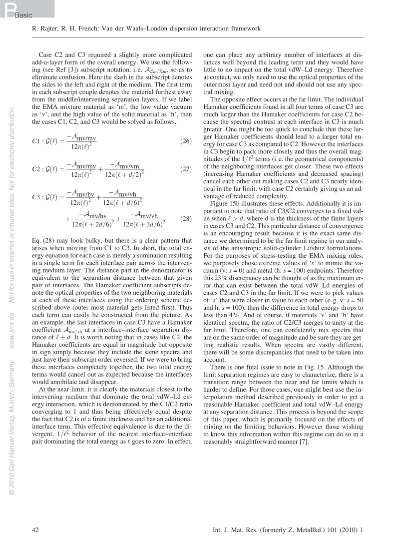
Case C2 and C3 required a slightly more complicatedadd-a-layer form of the overall energy. We use the follow-ing (see Ref [3]) subscript notation, i. e. ALm=Rm, so as toeliminate confusion. Here the slash in the subscript denotesthe sides to the left and right of the medium. The first termin each subscript couple denotes the material furthest awayfrom the middle/intervening separation layers. If we labelthe EMA mixture material as ‘m’, the low value vacuumas ‘v’, and the high value of the solid material as ‘h’, thenthe cases C1, C2, and C3 would be solved as follows.

C1 : Gð‘Þ ¼�Amv/mv12pð‘Þ2

ð26Þ

C2 : Gð‘Þ ¼�Amv/mv12pð‘Þ2

þ�Amv/vm

12pð‘þ d=2Þ2ð27Þ

C3 : Gð‘Þ ¼�Amv/hv12pð‘Þ2

þ�Amv/vh

12pð‘þ d=6Þ2

þ�Amv/hv

12pð‘þ 2d=6Þ2þ

�Amv/vh12pð‘þ 3d=6Þ2

ð28Þ

Eq. (28) may look bulky, but there is a clear pattern thatarises when moving from C1 to C3. In short, the total en-ergy equation for each case is merely a summation resultingin a single term for each interface pair across the interven-ing medium layer. The distance part in the denominator isequivalent to the separation distance between that givenpair of interfaces. The Hamaker coefficient subscripts de-note the optical properties of the two neighboring materialsat each of these interfaces using the ordering scheme de-scribed above (outer most material gets listed first). Thuseach term can easily be constructed from the picture. Asan example, the last interfaces in case C3 have a Hamakercoefficient Amv=vh at a interface–interface separation dis-tance of ‘þ d. It is worth noting that in cases like C2, theHamaker coefficients are equal in magnitude but oppositein sign simply because they include the same spectra andjust have their subscript order reversed. If we were to bringthese interfaces completely together, the two total energyterms would cancel out as expected because the interfaceswould annihilate and disappear.

At the near-limit, it is clearly the materials closest to theintervening medium that dominate the total vdW–Ld en-ergy interaction, which is demonstrated by the C1/C2 ratioconverging to 1 and thus being effectively equal despitethe fact that C2 is of a finite thickness and has an additionalinterface term. This effective equivalence is due to the di-vergent, 1=‘2 behavior of the nearest interface–interfacepair dominating the total energy as ‘ goes to zero. In effect,

one can place any arbitrary number of interfaces at dis-tances well beyond the leading term and they would havelittle to no impact on the total vdW–Ld energy. Thereforeat contact, we only need to use the optical properties of theoutermost layer and need not and should not use any spec-tral mixing.

The opposite effect occurs at the far limit. The individualHamaker coefficients found in all four terms of case C3 aremuch larger than the Hamaker coefficients for case C2 be-cause the spectral contrast at each interface in C3 is muchgreater. One might be too quick to conclude that these lar-ger Hamaker coefficients should lead to a larger total en-ergy for case C3 as compared to C2. However the interfacesin C3 begin to pack more closely and thus the overall mag-nitudes of the 1=‘2 terms (i. e. the geometrical components)of the neighboring interfaces get closer. These two effects(increasing Hamaker coefficients and decreased spacing)cancel each other out making cases C2 and C3 nearly iden-tical in the far limit, with case C2 certainly giving us an ad-vantage of reduced complexity.

Figure 15b illustrates these effects. Additionally it is im-portant to note that ratio of C3/C2 converges to a fixed val-ue when ‘ > d, where d is the thickness of the finite layersin cases C3 and C2. This particular distance of convergenceis an encouraging result because it is the exact same dis-tance we determined to be the far limit regime in our analy-sis of the anisotropic solid-cylinder Lifshitz formulations.For the purposes of stress-testing the EMA mixing rules,we purposely chose extreme values of ‘s’ to mimic the va-cuum (v: s = 0) and metal (h: s = 100) endpoints. Thereforethis 23% discrepancy can be thought of as the maximum er-ror that can exist between the total vdW–Ld energies ofcases C2 and C3 in the far limit. If we were to pick valuesof ‘s’ that were closer in value to each other (e. g. v: s = 50and h: s = 100), then the difference in total energy drops toless than 4%. And of course, if materials ‘v’ and ‘h’ haveidentical spectra, the ratio of C2/C3 merges to unity at thefar limit. Therefore, one can confidently mix spectra thatare on the same order of magnitude and be sure they are get-ting realistic results. When spectra are vastly different,there will be some discrepancies that need to be taken intoaccount.

There is one final issue to note in Fig. 15. Although thelimit separation regimes are easy to characterize, there is atransition range between the near and far limits which isharder to define. For those cases, one might best use the in-terpolation method described previously in order to get areasonable Hamaker coefficient and total vdW–Ld energyat any separation distance. This process is beyond the scopeof this paper, which is primarily focused on the effects ofmixing on the limiting behaviors. However those wishingto know this information within this regime can do so in areasonably straightforward manner [7].



BBasicW

2010

Car

lHan

ser

Ver

lag,

Mun

ich,

Ger

man

yw

ww

.ijm

r.de

Not

for

use

inin

tern

etor

intr

anet

site

s.N

otfo

rel

ectr

onic

dist

ribut

ion.

027-042 ijmr 110250 27. - Case School of Engineering

Documents

Transcript of 027-042 ijmr 110250 27. - Case School of Engineering