01$.2#)%&'34.5# · 2013-06-28 · 8 " 1 )" 2 = " $ '> ? 8 (9 9 : ; < ?! r9@ "%-b' 2"%4,$"2"#)' .4'...
69
General Introduction to Experimental Design Eugenia Migliavacca
Transcript of 01$.2#)%&'34.5# · 2013-06-28 · 8 " 1 )" 2 = " $ '> ? 8 (9 9 : ; < ?! r9@ "%-b' 2"%4,$"2"#)' .4'...

General Introduction to Experimental Design
Eugenia Migliavacca
SIB BCF 2September 06
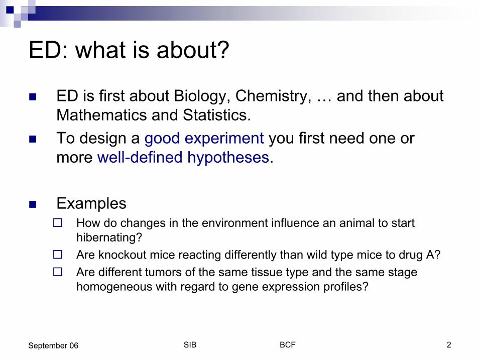
ED: what is about?
! ED is first about Biology, Chemistry, … and then about Mathematics and Statistics.
! To design a good experiment you first need one or more well-defined hypotheses.
! Examples" How do changes in the environment influence an animal to start
hibernating?" Are knockout mice reacting differently than wild type mice to drug A?" Are different tumors of the same tissue type and the same stage
homogeneous with regard to gene expression profiles?
SIB BCF 3September 06
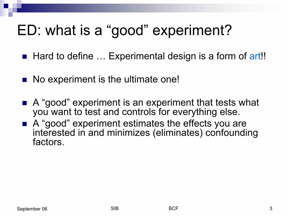
ED: what is a “good” experiment?
! Hard to define … Experimental design is a form of art!!
! No experiment is the ultimate one!
! A “good” experiment is an experiment that tests what you want to test and controls for everything else.
! A “good” experiment estimates the effects you are interested in and minimizes (eliminates) confounding factors.

SIB BCF 4September 06
ED: what is a “good” experiment?
! A c"n$"%n&in( $*c+"r or -*ri*.le is a "hidden" variable in a statistical or research model that affects the variables in question but is not known or acknowledged, and thus (potentially) distorts the resulting data. This hidden third variable causes the two measured variables to falsely appear to be correlated, or to be in a "causal"relation.
! An example would be a study of coffee drinking and lung cancer. If cigarette smokers are more likely to also be coffee drinkers, and the study measures coffee drinking but not smoking, the study may find that coffee drinking is associated with lung cancer which may or may not be true.
SIB BCF 5September 06
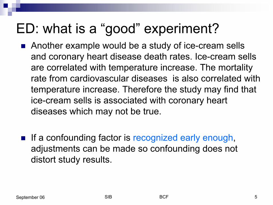
ED: what is a “good” experiment?! Another example would be a study of ice-cream sells
and coronary heart disease death rates. Ice-cream sells are correlated with temperature increase. The mortality rate from cardiovascular diseases is also correlated with temperature increase. Therefore the study may find that ice-cream sells is associated with coronary heart diseases which may not be true.
! If a confounding factor is recognized early enough, adjustments can be made so confounding does not distort study results.
SIB BCF 6September 06
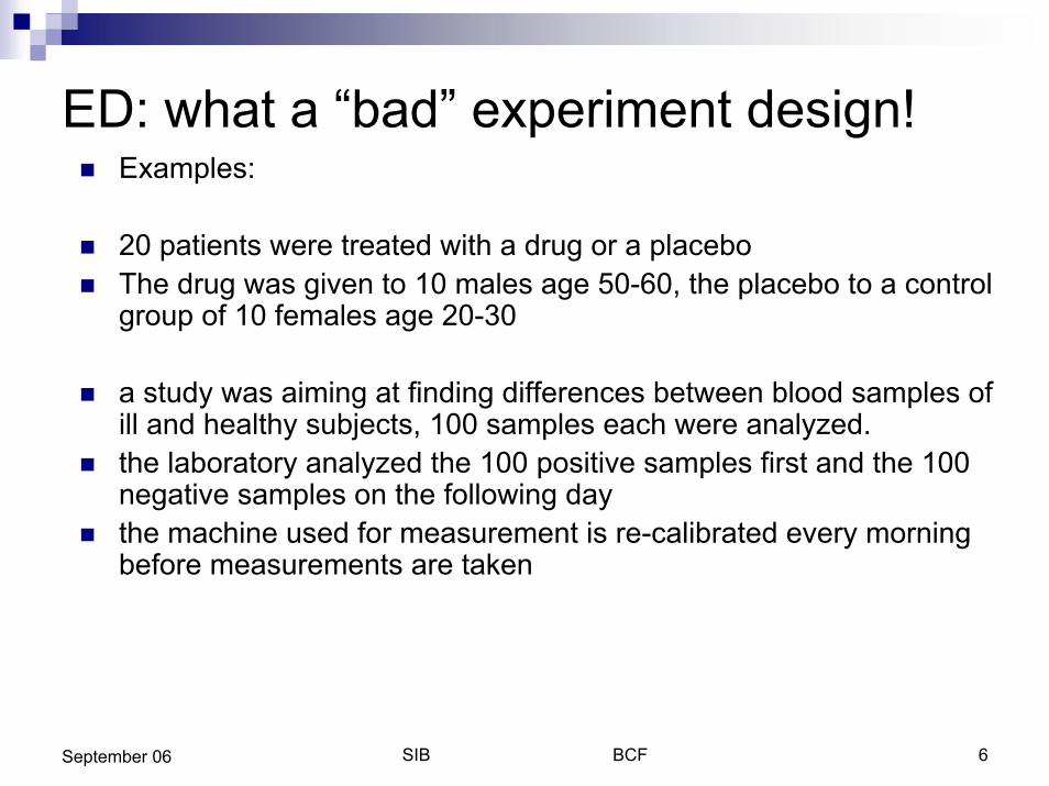
ED: what a “bad” experiment design!! Examples:
! 20 patients were treated with a drug or a placebo! The drug was given to 10 males age 50-60, the placebo to a control
group of 10 females age 20-30
! a study was aiming at finding differences between blood samples of ill and healthy subjects, 100 samples each were analyzed.
! the laboratory analyzed the 100 positive samples first and the 100 negative samples on the following day
! the machine used for measurement is re-calibrated every morning before measurements are taken
SIB BCF 7September 06
ED: what a “bad” experiment design!! Examples:
! If we are interested in the differences in gene expression between tumor and nonneoplastic mucosa in colon cancer patients
! we performed all tumor samples one day in laboratory A and all mucosa samples week later in laboratory B
! Which conclusions can we draw from such experiments?! Can we answer to the questions of interest? ! Can we generalize our conclusion?
! Any reasonably skeptical person would doubt the validity of whatever conclusions would be drawn from these study!
! For some bad experimental designs there are NO statistical fixing.

SIB BCF 8September 06
ED: Three Decisions
! In planning most of the experiments, you have to decide1. what measurement to make (the responses)2. what conditions to study (the treatments)3. what experimental material to use (the units)
! ExampleHow do changes in the environment influence an animal to start hibernating?What is the effect of changing day length (treatment) on the concentration of sodium pump enzyme (response) in the golden hamster (brain, unit)?
SIB BCF 9September 06
ED: Three Sources of Variability
! Variability due to the conditions of interest (wanted)! Variability in the measurement process (unwanted and
unavoidable)! Variability in the experimental material (unwanted and
unavoidable)! A good design will let you estimate the amount of
variability due to each source.! We need biological and statistical thinking to reach a
good ED!

SIB BCF 10September 06
ED: Three Kinds of Variability
! Planned, systematic variability (good).! Chance-like variability (tolerable); it includes
experimental error or chance error, NB: error ! mistake.chance error = observed value (from a sample) –“true” value (from population)
! Unplanned, systematic variability (bad); it includes bias and it can lead to wrong conclusions.
! Example: survey on food habits and weight of UNIL students.
! There are two main strategies: blocking and random assignment.
SIB BCF 11September 06
ED: Three Kind of Variability
! Say we sample from a population in order to estimate the population mean of some (numerical) variable of interest (e"#" weight, height, number of children, etc.)
! We could use the sample mean as our guess for the unknown value of the population mean
! Our (observed) sample mean is very unlikely to be exactly equal to the (unknown) population mean just due to chance variation in sampling
! Thus, it is useful to quantify the likely size of this chance variation (also called ‘chance error’ or ‘sampling error’, as distinct from ‘nonsampling errors’ such as bias)

SIB BCF 12September 06
ED First Principle: Random Assignment! In planning an experiment, any assigning that would
otherwise be haphazard (without an obvious plan) should be done using a chance device, random permutation.
! Example: choose mice from cages to assign them to hyper or hypocaloric diets. Randomized clinical studies.
! Randomizing converts unplanned, systematic variability into planned, chance-like variability.
! Especially in small samples one treatment might be more “lucky” in the randomized selection of the units to which it is applied. There is no foolproof method of allocation but methods that attempt at making the allocation as “fair” as possible.
SIB BCF 13September 06
ED Second Principle: Blocking! First subdivide your experimental material into groups
(blocks) of similar units; then assign conditions to units separately within each block. Each block should include (roughly) equal numbers for each treatment .
Units are similar if they are likely to give similar values for your measurement.
! Because response from different units varies even if the units are treated identically, must apply each treatment to several different units.Otherwise the results will be ambiguous, in that we will not be able to discern whether a difference is caused by the treatment or merely reflects differences (known or unknown) between the units
SIB BCF 14September 06
ED Second Principle: Blocking
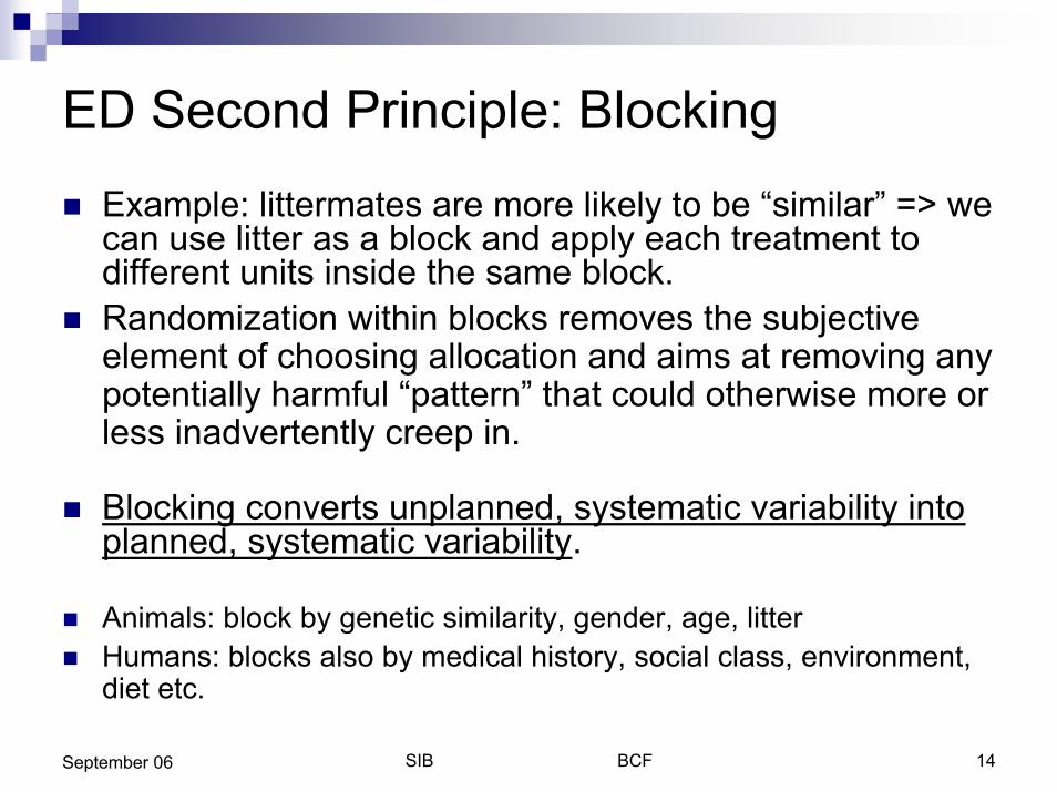
! Example: littermates are more likely to be “similar” => we can use litter as a block and apply each treatment to different units inside the same block.
! Randomization within blocks removes the subjective element of choosing allocation and aims at removing any potentially harmful “pattern” that could otherwise more or less inadvertently creep in.
! Blocking converts unplanned, systematic variability into planned, systematic variability.
! Animals: block by genetic similarity, gender, age, litter! Humans: blocks also by medical history, social class, environment,
diet etc.

SIB BCF 15September 06
ED Second Principle: Blocking ! Example: two blocks! Agricultural experiment, crop yield! Two different sorts of potatoes! Control over the quality of the soil: in one (believed
to be homogeneous) field use half for sort A and half for B, the same on a second block (believed to be homogeneous)
!loc% '!loc% (

SIB BCF 16September 06
Example: two blocks
!loc% '!loc% (
T*pe A
T*pe !
! Is this a good design ?

SIB BCF 17September 06
Example: two blocks
Assume some values for the parameters! ! = 120 kg ; ! "1 = + 10 kg ; "2 = - 10 kg ; ! #1 = + 25 kg ; #2 = - 25 kg ;
This would mean that the mean yields are:! Type A in block 1 : E[Y1] = ! $%"1 $%#1 = 155 kg! Type A in block 2 : E[Y1] = ! $%"1 $%#2 = 105 kg! Type B in block 1 : E[Y1] = ! $%"2 $%#1 = 135 kg! Type B in block 2 : E[Y1] = ! $%"2 $%#2 = 85 kg! ! = 120 kg is the average of the 4 cell averages
T*pe A
T*pe !
!loc% '!loc% (
&''
&('&)' *'
& +

SIB BCF 18September 06
Replication
!loc% '!loc% (
Here there are 5 replicas for each treatment in the first block and 8 in the second.
! In the previous example there is no replication, but it is needed to estimate the scale of random effects / measurement errors, therefore the fields are further subdivided into smaller areas and the choice of sort of potatoes to be planted is randomized inside the two main blocks.
SIB BCF 19September 06
Philosophy of Analysis
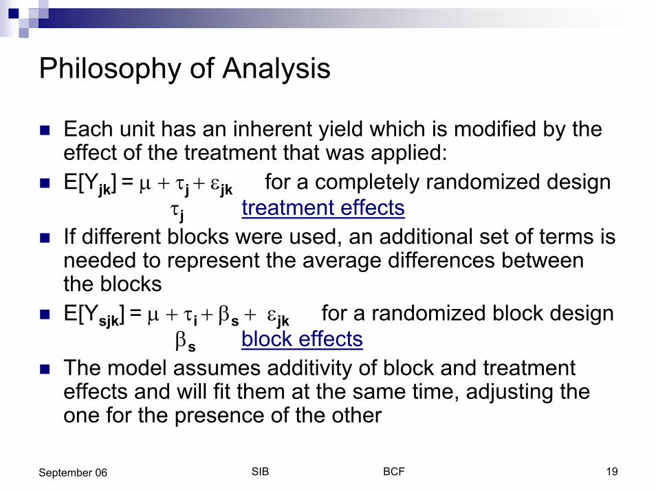
! Each unit has an inherent yield which is modified by the effect of the treatment that was applied:
! E[Y34] = !%$%"3 $%,34 for a completely randomized design"3 treatment effects
! If different blocks were used, an additional set of terms is needed to represent the average differences between the blocks
! E[Y534] = !%$%"i $%#5 $%%,34 for a randomized block design#5 block effects
! The model assumes additivity of block and treatment effects and will fit them at the same time, adjusting the one for the presence of the other

SIB BCF 20September 06
ED Third Principle: Factorial Crossing
! If you want to compare the effects of two or more set of conditions in the same experiment, take the set of all possible combination as your condition. Example 2x2 factorial design, 22.
! Factors: a) genotype b) drug administration
! Levels: wild-type mutant placebo active compound! Four possible combinations:
WT-Pl, WT-AC, Mu-Pl, Mu-AC
SIB BCF 21September 06
ED Third Principle: Factorial Crossing
! Compare two (or more) sets of conditions in the sameexperiment.
! Designs with factorial treatment structure allow you to measure interaction between two (or more) sets of conditions that influence the response.
! Factorial designs may be either observational or experimental.

SIB BCF 22September 06
Different types of 2-factor factorial designs
1. 2 experimental factors – you randomize treatments to each unit.
2. 2 observational factors – you cross-classify your populations into groups and get a sample from each population.
3. 1 experimental and 1 observational factor – you get a sample of units from each population, then use randomization to assign levels of the experimental factor (treatments), separately within each sample.
SIB BCF 23September 06
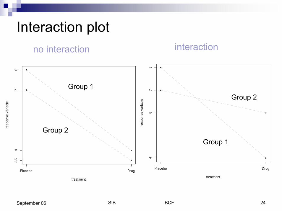
Interaction! Interaction is very common (and very important)
in science.! Interaction is a difference of differences"! Interaction is present if the effect of one factor
is different for different levels of the other factor! Main effects can be difficult to interpret in the
presence of interaction.
SIB BCF 24September 06
Interaction plotinteractionno interaction
Group 1
Group 2
Group 1
Group 2

SIB BCF 25September 06
Philosophy of Analysis
! Each unit has an inherent yield which is modified by the effect of the treatments that were applied and eventually by the interaction term:
! E[Y3i4] = !%$%-3 $%.i $ /4$,3i4-3 .i treatment effects/4 interaction effect

SIB BCF 26September 06
ED: basic example
! Determine the weight of A and BNB: each measurement is attached with an error of variance "2
! Method 1" Effort: 2 experiments
! weight A! weight B
" Precision: Var(A)=Var(B) = "2
! Method 2" Effort: 2 experiments
! weight A+B=S! weight A-B=D
" Precision: Var(A)=Var(B) = "2/2
A = (S+D)/2 2A=S+DVar(2A)=Var(S+D)=4Var(A)Var(S+D)= Var(S)+Var(D) if S and D are independentVar(S+D)=4Var(A)=2 "2
Var(A)=2/4 "2
SIB BCF 27September 06
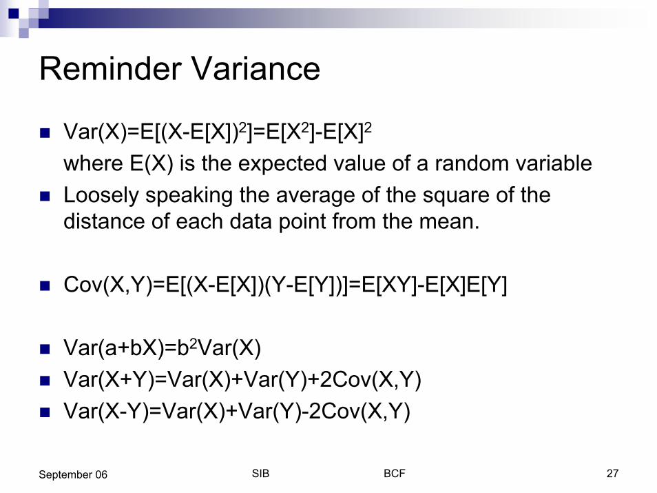
Reminder Variance
! Var(X)=E[(X-E[X])2]=E[X2]-E[X]2
where E(X) is the expected value of a random variable! Loosely speaking the average of the square of the
distance of each data point from the mean.
! Cov(X,Y)=E[(X-E[X])(Y-E[Y])]=E[XY]-E[X]E[Y]
! Var(a+bX)=b2Var(X)! Var(X+Y)=Var(X)+Var(Y)+2Cov(X,Y)! Var(X-Y)=Var(X)+Var(Y)-2Cov(X,Y)
SIB BCF 28September 06
Summary
! ED is first about Biology, Chemistry, … and then about Mathematics and Statistics.
! We need biological and statistical thinking to reach a good ED!
! A good ED will optimize of the ratio number of experiments/information obtained.

Introduction to Experimental Designfor Microarray Experiments
Eugenia Migliavacca

SIB BCF 30September 06
Considerations for MicroarrayExperiments
! &cienti)ic +Aims o) the e1periment4– Specific questions and priorities– How will the experiments answer the questions
! 5ractical +8o#istic4" Types of mRNA samples" Source and amount of material (tissues, cell lines)
! Other Information" Experimental process prior to hybridization " Controls planned: positive, negative, etc." Verification method: Northern, RT-PCR, etc.

SIB BCF 31September 06
Design Aspects! Arra9 8a9out
– Which probe sequences are printed– Spatial position
! ;eneral consi<erations– Replication / Sample size– Randomization– Blocking
! Allocation o) samples to sli<es – Treatment vs control, Multiple treatments– Factorial – Time course

SIB BCF 32September 06
Replication
! Why?"To reduce variability"To increase generalizability
! What is it?"Duplicate spots"Duplicate sli<es
– Technical replicates – usually less desirable– >iolo#ical replicates

SIB BCF 33September 06
Sample Size
! More difficult than usual, as there are 1,000s of possible changes, each with its own SD
! Acceptable )alse positi?e rate! Desired po@er (probability of detecting an effect
of at least the specified size)! Aariance of individual measurements (X)! B))ect siCe+s4 to be detected (X)
SIB BCF 34September 06
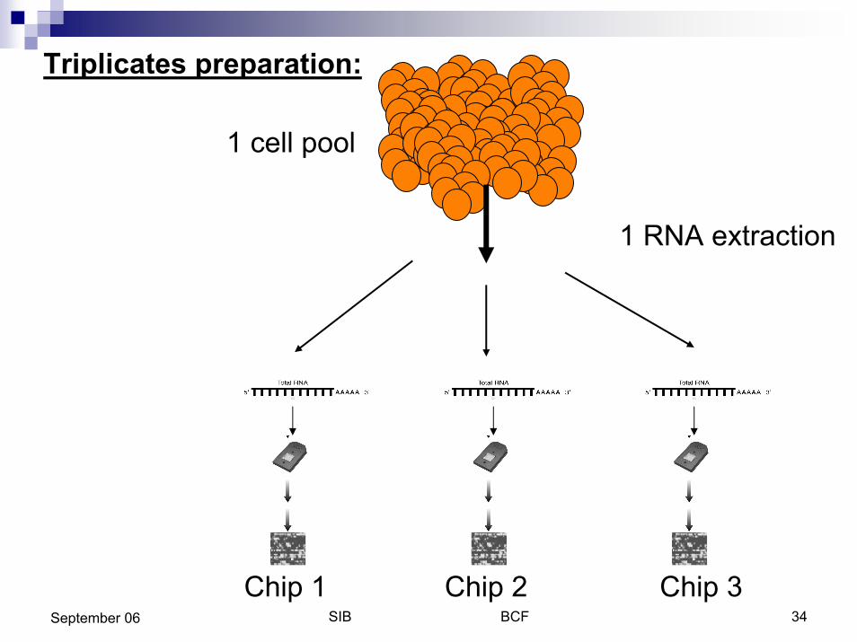
6riplic*+e5 prep*r*+i"n:
1 cell pool
1 RNA extraction
Chip 1 Chip 2 Chip 3

SIB BCF 35September 06
6riplic*+e5 prep*r*+i"n:
3 RNA extractions
1 cell pool
Chip 1 Chip 2 Chip 3
SIB BCF 36September 06
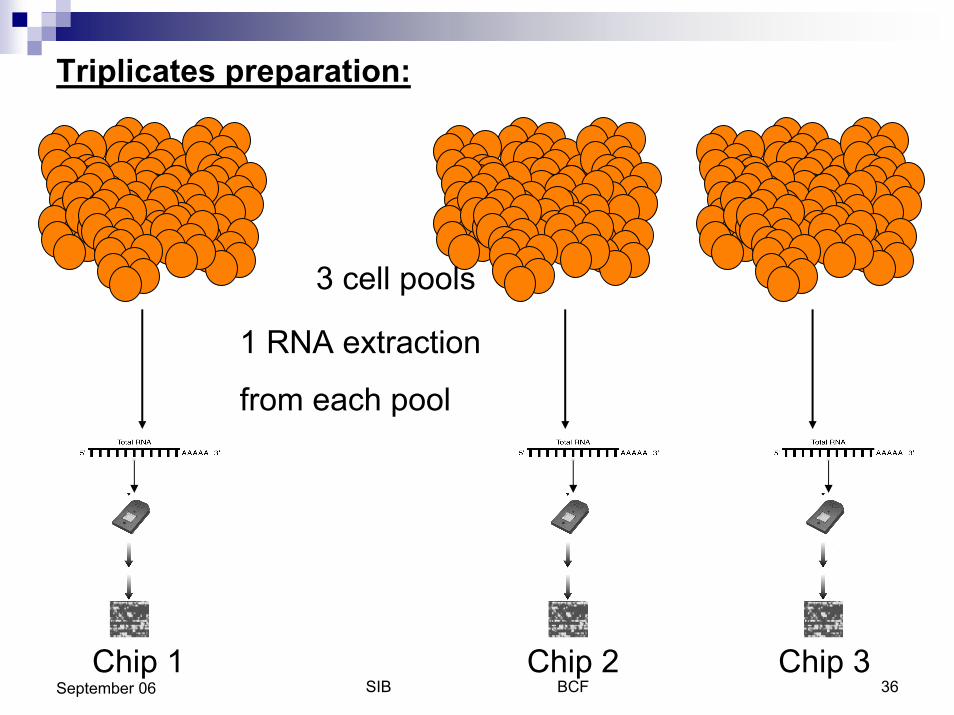
6riplic*+e5 prep*r*+i"n:
3 cell pools
1 RNA extraction
from each pool
Chip 1 Chip 2 Chip 3
SIB BCF 37September 06
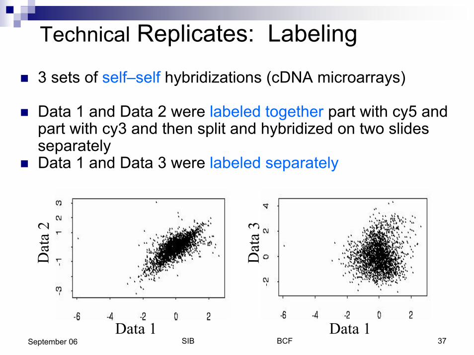
Technical Replicates: Labeling
! 3 sets of self–self hybridizations (cDNA microarrays)
! Data 1 and Data 2 were labeled together part with cy5 and part with cy3 and then split and hybridized on two slides separately
! Data 1 and Data 3 were labeled separately
Data ' Data '
Dat
a (
Dat
a 1
SIB BCF 38September 06
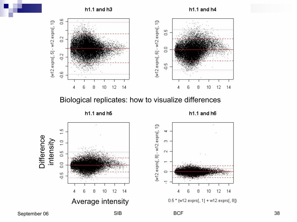
Biological replicates: how to visualize differences
Average intensity
Diff
eren
ce
inte
nsity

SIB BCF 39September 06

SIB BCF 40September 06
Graphical representation
AerticesD mRNA samplesB<#esD hybridizationDirectionD dye assignment
9:; 5*<ple
9:= 5*<ple
SIB BCF 41September 06
Comparing samples
! The structure of the graph determines which effects can be estimated and the precision of the estimates
! Two mRNA samples can be compared only if there is a path joining the corresponding two vertices
! The precision of the estimated contrast then depends on the numFer o) paths joining the two vertices and is inversely related to the len#th o) the paths

SIB BCF 42September 06
Natural design choice61 62 6; 64
Gase HD Ieanin#)ul Fiolo#ical control +G4Samples: Liver tissue from four mice treated by a drug.Question 1: Which genes respond differently between T and C?Question 2: Which genes respond similarly across two or more
treatments relative to control.Gase JD Kse o) uni?ersal re)erence +Re)4Samples: Different tumor samples.Question: Can we discover tumor subtypes?
61
?e$
62 6n-1 6n
9

SIB BCF 43September 06
Treatment vs ControlTwo samplese"#" KO vs. WT or mutant vs. WT
6 96 ?e$9 ?e$
Direct Indirect
*-er*(e (l"( (6/9)) l"( (6 / ?e$) D l"( (9 / ?e$ )
0( 2( (0(
Var((y1-y2)/2) = 1/4Var(y1-y2) =1/4*[Var(y1)+Var(y2)]=1/4*2 0+ 1%0+ /2
Var(y1-y2) = Var(y1)+Var(y2)= 2 0+
SIB BCF 44September 06
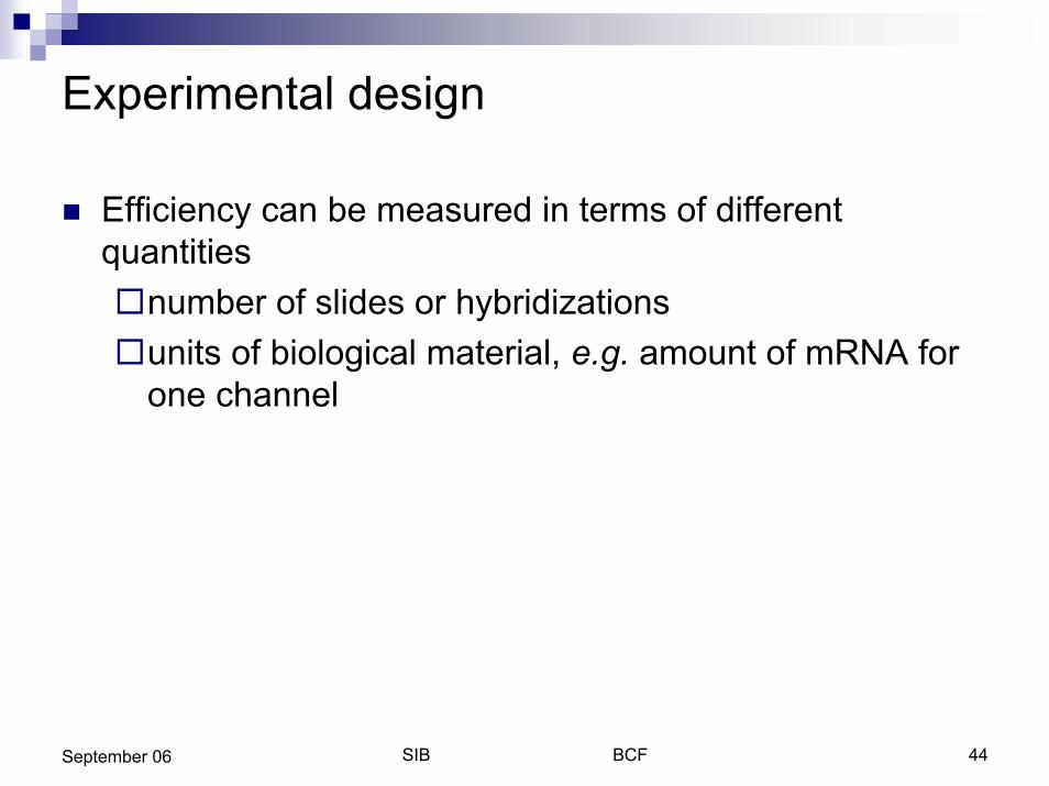
Experimental design
! Efficiency can be measured in terms of different quantities"number of slides or hybridizations"units of biological material, e"#" amount of mRNA for
one channel
SIB BCF 45September 06
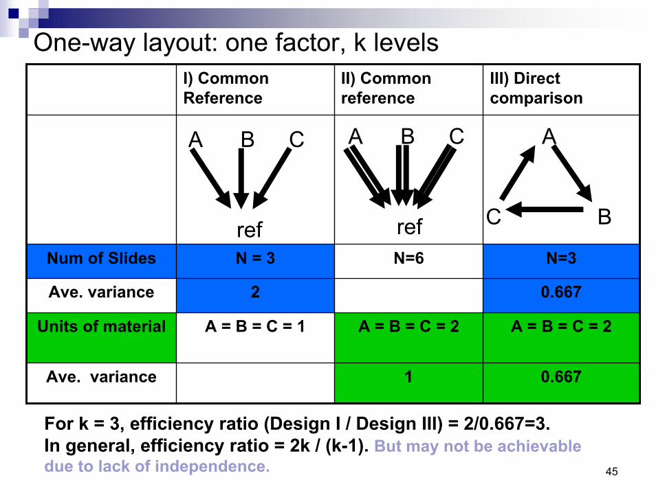
One-way layout: one factor, k levelsE) 9"<<"n ?e$erence
EE) 9"<<"n re$erence
EEE) Firec+ c"<p*ri5"n
G%< "$ Hli&e5 G = ; G=J G=;
A-e. -*ri*nce 2 0.JJN
Oni+5 "$ <*+eri*l A = B = 9 = 1 A = B = 9 = 2 A = B = 9 = 2
A-e. -*ri*nce 1 0.JJN
C B
A
ref
CBA
ref
CBA
Q"r 4 = ;R e$$icienc: r*+i" (Fe5i(n E / Fe5i(n EEE) = 2/0.JJN=;.En (ener*lR e$$icienc: r*+i" = 24 / (4-1). B%+ <*: n"+ .e *cSie-*.le &%e +" l*c4 "$ in&epen&ence.
SIB BCF 46September 06
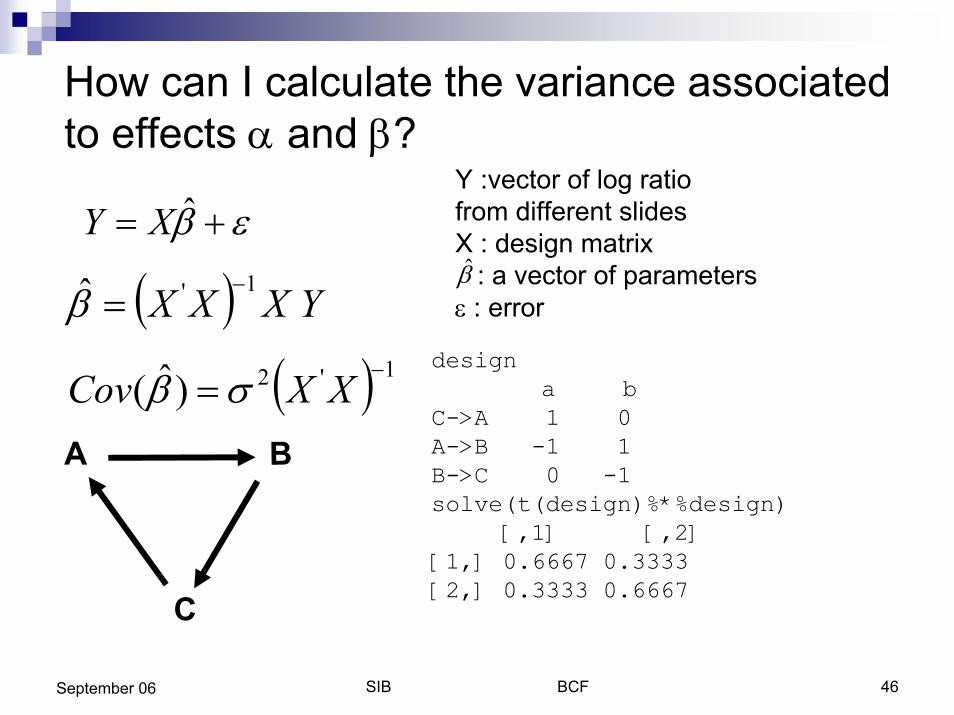
How can I calculate the variance associated to effects - and #?
,# $1 3XYY :vector of log ratio from different slidesX : design matrix
: a vector of parameters ,%: error#32 3 YXXX 3 '4 4
1#
2 3 '4(536 41 XXCov 0#
designa b
C->A 1 0A->B -1 1B->C 0 -1solve(t(design)%*%design)
[,1] [,2][1,] 0.6667 0.3333[2,] 0.3333 0.6667
A B
9
SIB BCF 47September 06
Fe5i(n E
Fe5i(n EEEA B
9
A
?e$
B 9
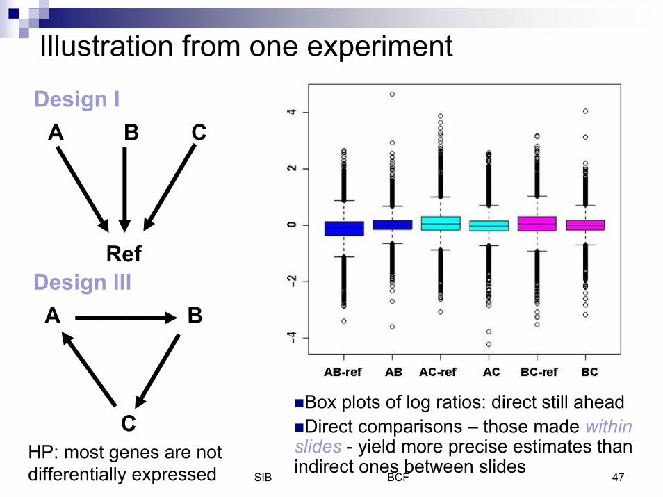
Illustration from one experiment
!Box plots of log ratios: direct still ahead!Direct comparisons – those made @ithin sli<es - yield more precise estimates than indirect ones between slides
HP: most genes are not differentially expressed

SIB BCF 48September 06
Allocating samples
! The main issue with 2-color arrays is the use of re)erence samples (typically labelled green, although not required to be)
! Standard statistical design principles can lead to more e))icient la9outs
! Use of <9eMs@aps for some types of experiments can also help ...
SIB BCF 49September 06
Dye Swap (Reverse Labeling)
! Some investigators suggest that all arrays should be performed both forward- and reverse- labeled, e.g. sample A1 Cy5, sample B1 Cy3; sample B1 Cy5 and sample A1 Cy3. USUALLY this is NOT NECESSARY.
! Balanced labeling is much more efficient than replicating hybridizations of the biological units with swapped dye labeling. Example of balanced labeling sample A1 Cy5, sample B1 Cy3; sample B2 Cy5 and sample A2 Cy3; sample A3 Cy5, sample B3 Cy3; sample B4 Cy5 and sample A4 Cy3.
SIB BCF 50September 06
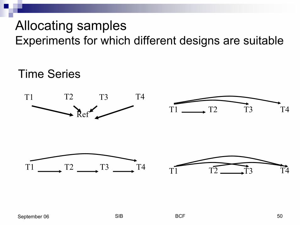
Allocating samplesExperiments for which different designs are suitable
Time Series
T( T7T' T1T( T1 T7T'Re9
T( T1 T7T' T( T1 T7T'
SIB BCF 51September 06
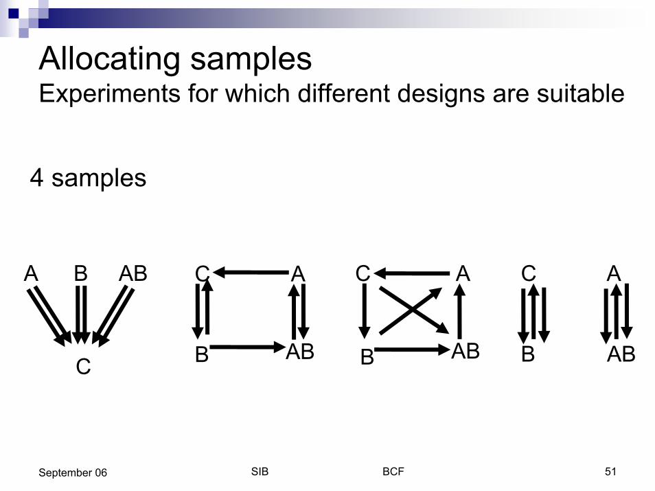
Allocating samplesExperiments for which different designs are suitable
4 samples
ABBA
C B
C
AB
A
B
C
AB
A
B
C
AB
A
SIB BCF 52September 06
Randomization and Blocking
! Usually more of an issue in lar#er e1periments" done with many samples, " by different technicians, " over a long period of time, " etc"
BIAS
SIB BCF 53September 06
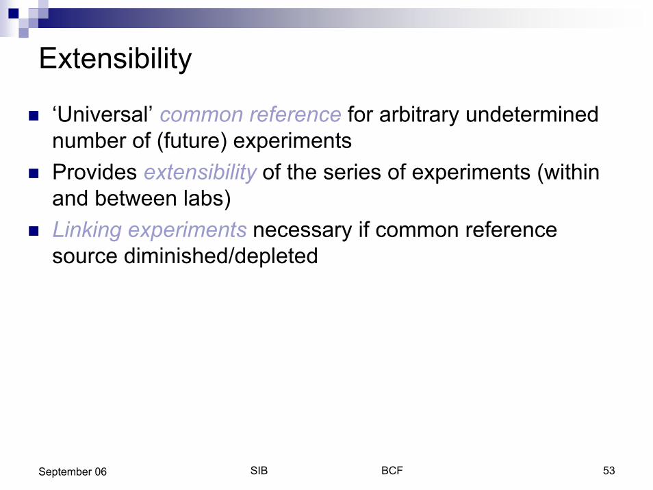
Extensibility
! ‘Universal’ common re)erence for arbitrary undetermined number of (future) experiments
! Provides e1tensiFilit9 of the series of experiments (within and between labs)
! 8inNin# e1periments necessary if common reference source diminished/depleted
SIB BCF 54September 06
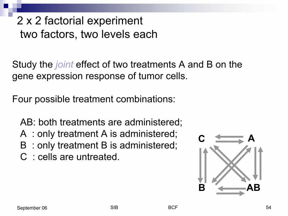
2 x 2 factorial experimenttwo factors, two levels each
9 A
B AB
Study the Ooint effect of two treatments A and B on the gene expression response of tumor cells.
Four possible treatment combinations:
AB: both treatments are administered;A : only treatment A is administered;B : only treatment B is administered;C : cells are untreated.
SIB BCF 55September 06
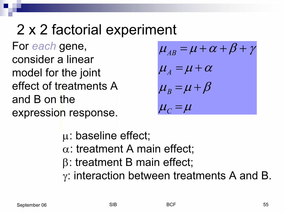
2 x 2 factorial experimentFor each gene, consider a linear model for the joint effect of treatments A and B on the expression response.
!AB 1 !%$%-%$%#%$ /!A 1 !%$%-!B %1%!%$%#!C %1%!
!: baseline effect;-: treatment A main effect; #: treatment B main effect;/: interaction between treatments A and B.

SIB BCF 56September 06
2 x 2 factorial experiment!C
!AB!B
Log-ratio M for hybridization
estimates
9 A
B AB
!A
A AB
!AB 4!A 1%#%$ /
Log-ratio M for hybridization
estimates!C %1%!!A 1 !%$%-!B %1%!%$%#!AB 1 !%$%-%$%#%$ /
A B
!B 4!A 1%#%4%-

SIB BCF 57September 06
Experimental design
! In addition to experimental constraints, design decisions should be guided by the knowledge of which effects are of greater interest to the investigator (which main effects, which interactions)
! The experimenter should thus decide on the comparisons for which he wants the most precision and these should be made @ithin sli<es to the extent possible.

SIB BCF 58September 06
Experiment for which a number of designs are suitable for use
4 samples Which is the best design?
ABBA
C B
C
AB
A
B
C
AB
A
B
C
AB
A
SIB BCF 59September 06
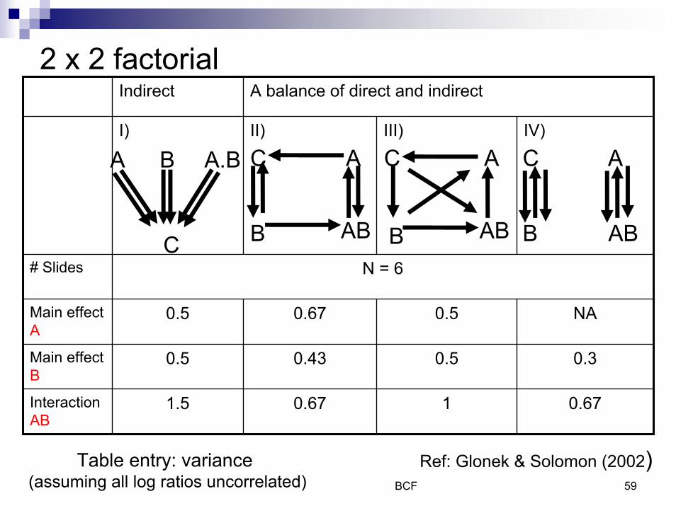
Indirect A balance of direct and indirect
I) II) III) IV)
0.67
0.43
0.67
# Slides N = 6
Main effect A
0.5 0.5 NA
Main effect B
0.5 0.5 0.3
Interaction AB
1.5 1 0.67
C
A.BBA
B
C
AB
A
B
C
AB
A
B
C
AB
A
2 x 2 factorial
Ref: Glonek & Solomon (2002)Table entry: variance (assuming all log ratios uncorrelated)
SIB BCF 60September 06
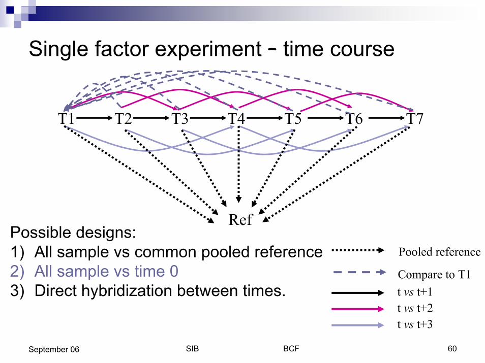
Single factor experiment – time course
Possible designs:1) All sample vs common pooled reference2) All sample vs time 03) Direct hybridization between times.
:oole; re9erence
T( T7 T> T? T@T1T'
Re9
Aompare to T't vs tC't vs tC(t vs tC1
SIB BCF 61September 06
Time Course Experiments
! Number and placement of time points! Which differences are of highest interest (e.g.
between initial time and later times, between adjacent times)
! Number of slides available

SIB BCF 62September 06
t vs t+1 t vs t+2 t vst+3Design choices in time series
Entry: variance
A) T1 as common reference 1 2 2 1 2 1 1.=N=3
N=4
B) Direct Hybridization 1 1 1 2 2 ; 1.JN
T1T2 T2T3 T3T4 T2T4 T1T4
2 2
1.67
1
.75
1.67
2
1
.75.75
1 .75
2
.67
.75
.75
2
.67
.75
1
T1T3
Ave
C) Common reference 2 2
D) T1 as common ref + more .67 1.06
E) Direct hybridization choice 1 1 .83
F) Direct Hybridization choice 2 .75 .83
T( T1 T7T'
T( T1 T7T'Re9
T( T1 T7T'
T( T1 T7T'
T( T1 T7T'
T( T1 T7T'
SIB BCF 63September 06
Pooling of Samples
! Although the pooled sample approach may be applicable for preliminary screening, the approach does not provide a valid basis for biological conclusions.
! Biological replication is necessary.! Biological replication can be achieved by assaying
individual samples or independent pools of distinct samples.
! Disadvantages:" pooling permits one sample (or a few) to dominate the outcome;" looses the ability to estimate the between-sample variation.

SIB BCF 64September 06
Reminder: False Positive and False Negative
not rejected rejected
true H #specificity
XType I error (False +) -
false H XType II error (False -) #
#Power 1 - #;sensitivity
DecisionTruth
SIB BCF 65September 06
Reminder: - and 1-#
! The significance level (-) is the probability of concluding that a gene is differentially expressed between two classes when in fact the means are the same (.1(3.
! The statistical power (1-#) is the probability of obtaining statistical significance in comparing gene expression between the two classes when the true difference in mean expression levels between the classes is ..
SIB BCF 66September 06
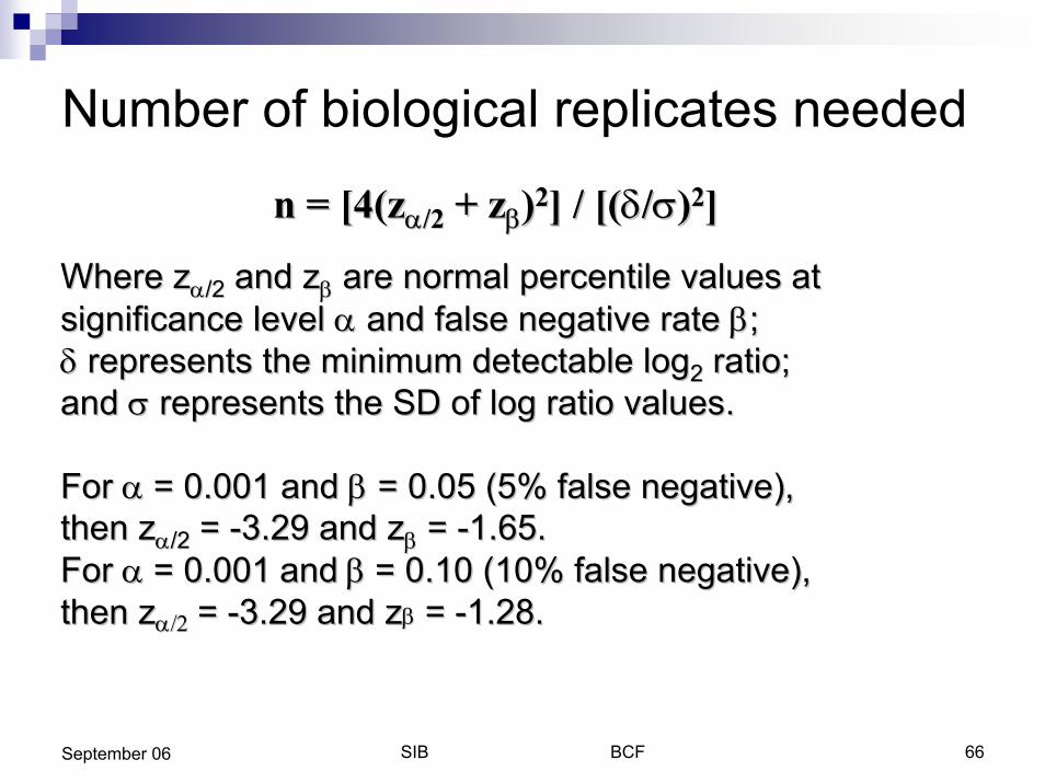
Number of biological replicates needed
n = [4(zn = [4(z--/2/2 + z+ z##))22] / [(] / [(..//00))22]]
Where zWhere z--/2/2 and and zz## are normal percentile values at are normal percentile values at significance level significance level -- and and falsefalse negative rate negative rate ##; ; .. represents the minimum detectable logrepresents the minimum detectable log22 ratioratio;;and and 00 represents the SD of log ratio valuesrepresents the SD of log ratio values..
For For -%-%= 0.001 and = 0.001 and ## = 0.05 (5% false negative), = 0.05 (5% false negative), then zthen z--/2/2 = = --3.29 and 3.29 and zz## = = --1.65.1.65.For For -%-%= 0.001= 0.001 andand #%#%= 0.10 (10% false negative),= 0.10 (10% false negative),then zthen z-5+-5+ = = --3.29 and 3.29 and zz## = = --1.28.1.28.
SIB BCF 67September 06
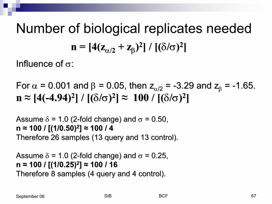
Number of biological replicates neededn = [4(zn = [4(z--/2/2 + z+ z##))22] / [(] / [(..//00))22]]
Influence of Influence of 00::
For For -%-%= 0.001 and = 0.001 and ## = 0.05, then z= 0.05, then z--/2/2 = = --3.29 and 3.29 and zz## = = --1.65.1.65.n ! [4(n ! [4(--4.94)4.94)22] / [(] / [(..//00))22] ! 100 / [(] ! 100 / [(..//00))22]]
Assume Assume .. = 1.0 (2= 1.0 (2--fold change) and fold change) and 00 = 0.50,= 0.50,n ! 100 / [(1/0.=0)n ! 100 / [(1/0.=0)22] ! 100 / 4 ] ! 100 / 4 ThereforeTherefore 26 samples (13 query and 13 control).26 samples (13 query and 13 control).
Assume Assume .. = 1.0 (2= 1.0 (2--fold change) and fold change) and 00 = 0.25,= 0.25,n ! 100 / [(1/0.2=)n ! 100 / [(1/0.2=)22] ! 100 / 1J ] ! 100 / 1J ThereforeTherefore 8 samples (4 query and 4 control).8 samples (4 query and 4 control).
SIB BCF 68September 06
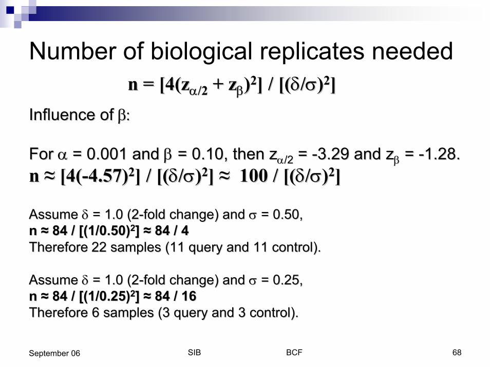
Number of biological replicates neededn = [4(zn = [4(z--/2/2 + z+ z##))22] / [(] / [(..//00))22]]
Influence of Influence of #6#6
For For -%-%= 0.001 and = 0.001 and ## = 0.10, then z= 0.10, then z--/2/2 = = --3.29 and 3.29 and zz## = = --1.28.1.28.n ! [4(n ! [4(--4.57)4.57)22] / [(] / [(..//00))22] ! 100 / [(] ! 100 / [(..//00))22]]
Assume Assume .. = 1.0 (2= 1.0 (2--fold change) and fold change) and 00 = 0.50,= 0.50,n ! V4 / [(1/0.=0)n ! V4 / [(1/0.=0)22] ! V4 / 4 ] ! V4 / 4 ThereforeTherefore 22 samples (11 query and 11 control).22 samples (11 query and 11 control).
Assume Assume .. = 1.0 (2= 1.0 (2--fold change) and fold change) and 00 = 0.25,= 0.25,n ! V4 / [(1/0.2=)n ! V4 / [(1/0.2=)22] ! V4 / 1J ] ! V4 / 1J ThereforeTherefore 6 samples (3 query and 3 control).6 samples (3 query and 3 control).

SIB BCF 69September 06
Summary
! Must satisfy scientific and physical constraints of the experiment.
! Balance of direct and indirect comparisons! Optimize precision of the estimates among
comparisons of interest.! It can save you a lot of time, money and heart-ache
to think carefully about experimental design issues before carrying out any experiments.