
01/20151 EPI 5344: Survival Analysis in Epidemiology Interpretation of Models March 17, 2015 Dr. N....
31
01/2015 1 EPI 5344: Survival Analysis in Epidemiology Interpretation of Models March 17, 2015 Dr. N. Birkett, School of Epidemiology, Public Health & Preventive Medicine, University of Ottawa
Transcript of 01/20151 EPI 5344: Survival Analysis in Epidemiology Interpretation of Models March 17, 2015 Dr. N....

101/2015
EPI 5344:Survival Analysis in
EpidemiologyInterpretation of Models
March 17, 2015
Dr. N. Birkett,School of Epidemiology, Public Health &
Preventive Medicine,University of Ottawa

2
Objectives
• Epidemiology often tries to determine risk associated
with ‘exposures’ or like events
• Various types of exposures– nominal
– ordinal
– count
– continuous
• Session looks at how to use these different types of
exposures in Cox models
• And, how to interpret the results01/2015

3
Nominal variables (1)
• Categories– Male/female– Occupation– City of residence
01/2015

4
Nominal variables (2)
• Can not be rank ordered– If you ‘impose’ a ranking, then you are defining a new
variable.– No intrinsic numerical value
• Even if they are commonly coded as 1/2, they are NOT NUMERIC
• Use of 1/2/3 coding dates back to early days of computers• Can assign letters or words to categories (e.g.
Male/Female)
– Usually analyzed using dummy variables• Indicator variables is a better term.
01/2015

5
Nominal variables (3)
• SAS must be aware that these variables are categories, not numbers– CLASS statement
• Indicator variables– ‘n’ response levels ‘n-1’ indicator variables– Why?
• The MLE equations are indeterminate if you include ‘n’ indicator variables.
01/2015

6
• Consider a two-level nominal variable– e.g. M/F
• Some possible IV codings:
• All (and many more) are possible.• #1 is the most commonly used
Nominal variables (4)
01/2015
Level #1 #2 #3 #4
1 (M)
2 (F)
Level #1 #2 #3 #4
1 (M) 1
2 (F) 0
Level #1 #2 #3 #4
1 (M) 1 1
2 (F) 0 -1
Level #1 #2 #3 #4
1 (M) 1 1 2
2 (F) 0 -1 1
Level #1 #2 #3 #4
1 (M) 1 1 2 10
2 (F) 0 -1 1 -18

7
• Suppose we have 3 levels (blue/green/red)
• Some possible Indicator Variable codings:
Nominal variables (5)
01/2015
Reference Effect OrthogonalPolynomial
Level #1X1 X2
#2X1 X2
#3X1 X2
1 (blue)
2 (green)
3 (red)
Level #1X1 X2
#2X1 X2
#3X1 X2
1 (blue) 1 0
2 (green) 0 1
3 (red) 0 0
Level #1X1 X2
#2X1 X2
#3X1 X2
1 (blue) 1 0 1 0
2 (green) 0 1 0 1
3 (red) 0 0 -1 -1
Level #1X1 X2
#2X1 X2
#3X1 X2
1 (blue) 1 0 1 0 -1.225 0.707
2 (green) 0 1 0 1 0 -1.414
3 (red) 0 0 -1 -1 1.225 0.707

8
Ordinal variables
• Still categorical (name) type data.
• But, there is an implicit ordering with the levels.– Disease severity
• mild, moderate, severe
– Rating scale• Agree/don’t care/disagree
• Interval data which has been categorized is really ‘ordinal’, not
interval.
• Commonly treat as nominal variables and ignore rank order
• Can use ordinal variables for trend or dose response analyses– Key issue: determining the spacing/numerical values to use
01/2015

9
Interval variables
• Has a meaningful ‘0’
• Can assume any value (perhaps within a range)– Infinite precision is possible.
• Examples– Blood pressure
– Cholesterol
– Income
• Usually treated as a continuous number
• Can categorize and then use ordinal methods– Can reduce measurement errors
– Useful for EDA to look for non-linear dose-response.
01/2015

10
Count variables
• The number of times an event has happened– # pregnancies
– # years of education
• Very common type of data in medical research
• Often regarded as continuous but isn’t really
• Can affect choice of model– Poisson distribution
01/2015

11
Parameter interpretation (1)
• Cox models Hazard Ratios not the hazard– Can not provide a direct estimates of S(t) or
h(t)– Needs additional assumptions or methods– Next week
• Cox model:• Contains no explicit intercept term
– That is the h0(t)
01/2015

12
Parameter interpretation (2)
• To explore Betas, we will use this form of
the Cox model:
• Start with 2-level nominal variable
• Consider 3 different coding approaches
01/2015

13
Parameter interpretation (3)
• We will have only one parameter.
01/2015
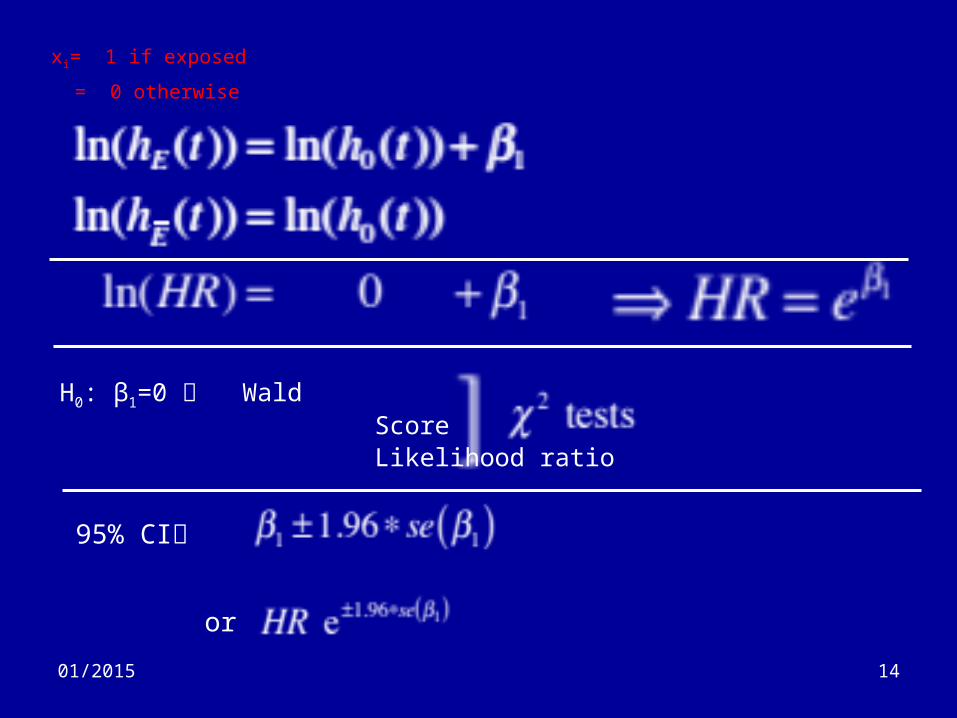
14
xi= 1 if exposed
= 0 otherwise
01/2015
H0: β1=0 Wald Score Likelihood ratio
95% CI
or

15
xi= 1 if exposed
= -1 otherwise
01/2015
• Changing the coding has changed the interpretation of
the Beta value
• ‘Effect’ coding compares each level to the mean effect
• ‘sort of’ since it is dependent on the number of subjects in
each level.

16
xi= 2 if exposed
= 1 otherwise
01/2015
• Changing the coding doesn’t always change the
interpretation of the Beta value
• Need to be aware of the coding used in order to correctly
interpret the model

17
Xi is continuous (interval)
Let’s consider the effect of changing the exposure by ‘1’ unit
01/2015
So,β1 relates to the HR for a 1 unit change in x1.What about an ‘s’ unit change?

18
Xi is continuous (interval)
Let’s consider the effect of changing the exposure by ‘s’ unit
01/2015
• SAS has an option to do this automatically.• Important to consider the level for a
‘meaningful’ change

1901/2015
Level #1X1 X2
#2X1 X2
#3X1 X2
1 (blue) 1 0 1 0 -1.225 0.707
2 (green) 0 1 0 1 0 -1.414
3 (red) 0 0 -1 -1 1.225 0.707

20
‘reference’ coding; level 3=ref
01/2015

21
‘effect’ coding
01/2015

22
• Effect coding– βi does NOT let you compare two levels
directly– Use ‘Reference Coding’ to do that
01/2015

23
‘orthogonal polynomial’ coding
01/2015

2401/2015
• Doesn’t look that useful or interesting • This coding can be used to test for linear
and quadratic effects in the dose-response relationship• Test β1 to look for a linear effect
• Test β2 to look for a quadratic effect
• Can be extended to higher orders if there are more levels.

25
Hypothesis testing (1)
• Does adding new variable(s) to a model lead to a
better model?– Test the statistical significance of the additional variables.
• Let’s start with 1 variable
• The likelihood is a function of the variable
– L = f(β1)
• To test β1=0, compare the likelihood of the model with
the MLE estimate to the ‘β1=0’ model
– f(0) vs. f(βMLE)01/2015

26
Hypothesis testing (2)
• As is common in statistics, this gives the best results if you:– Take logarithms– Multiple by -2
• Likelihood ratio test of H0: β1=0
01/2015

27
Hypothesis testing (3)
• Can extend to test the null hypothesis that ‘k’ parameters are simultaneously ‘0’.
• Likelihood ratio test of H0: β1=β2=….. βk=0
• Can be used to compare any two models– BUT, Models must be Nested or hierarchical
01/2015

28
Hypothesis testing (4)
• Nested– All of the variables in one model must be
contained in the other model• #1: x1, x2, x3, x4
• #2: x1, x2
– AND: Analysis samples must be identical• Watch for issues with missing data in extra variables
01/2015

29
Hypothesis testing (5)
• You can also do many of these tests using the Wald and Score approximations– Hopefully, you get the same answer
• Usually do (at least, in the same ballpark)
01/2015

30
Confidence Intervals (1)
• Always based on the Wald Approximation• First, determine 95% CI’s for the Betas
• Second, convert to 95% CI’s for the HR’s
01/2015

3101/2015