Datasets provided in spatstat

Adrian Baddeley, Rolf Turner and Ege Rubak

For spatstat version 1.41-1

This document is an overview of the spatial datasets that are provided in the spatstat package.To flick through a nice display of all the data sets that come with spatstat type demo(data). To

see information about a given data set, type help(name) where name is the name of the data set Toplot a given data set, type plot(name).

Datasets in spatstat are “lazy-loaded”, which means that they can be accessed simply by typingtheir name. Not all packages do this; in some packages you have to type data(name) in order to accessa data set.

1 List of datasets

1.1 Point patterns in 2D

Here is a list of the standard point pattern data sets that are supplied with the current installation ofspatstat:

1

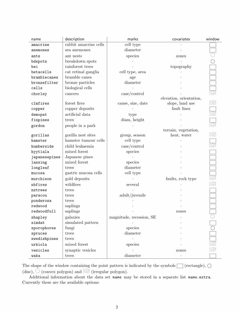
name description marks covariates window

amacrine rabbit amacrine cells cell type ·anemones sea anemones diameter ·ants ant nests species zonesbdspots breakdown spots · · ©bei rainforest trees · topographybetacells cat retinal ganglia cell type, area ·bramblecanes bramble canes age ·bronzefilter bronze particles diameter ·cells biological cells · ·chorley cancers case/control ·

clmfires forest fires cause, size, dateelevation, orientation,

slope, land usecopper copper deposits · fault lines

demopat artificial data type ·finpines trees diam, height ·gordon people in a park · ·

gorillas gorilla nest sites group, seasonterrain, vegetation,

heat, waterhamster hamster tumour cells cell type ·humberside child leukaemia case/control ·hyytiala mixed forest species ·japanesepines Japanese pines · ·lansing mixed forest species ·longleaf trees diameter ·mucosa gastric mucosa cells cell type ·murchison gold deposits · faults, rock type

nbfires wildfires several ·nztrees trees · ·paracou trees adult/juvenile ·ponderosa trees · ·redwood saplings · ·redwoodfull saplings · zones

shapley galaxies magnitude, recession, SE ·simdat simulated pattern · ·sporophores fungi species · ©spruces trees diameter ·swedishpines trees · ·urkiola mixed forest species ·vesicles synaptic vesicles · zoneswaka trees diameter ·

The shape of the window containing the point pattern is indicated by the symbols (rectangle), ©(disc), (convex polygon) and (irregular polygon).

Additional information about the data set name may be stored in a separate list name.extra.Currently these are the available options:

2

Name Contents

ants.extra field and scrub subregions;additional map elements; plotting function

bei.extra covariate imageschorley.extra incinerator location; plotting functiongorillas.extra covariate imagesnbfires.extra inscribed rectangleponderosa.extra data points of interest; plotting functionredwoodfull.extra subregions; plotting functionshapley.extra individual survey fields; plotting functionvesicles.extra anatomical regions

For demonstration and instruction purposes, raw data files are available for the datasets vesicles,gorillas and osteo.

1.2 Other Data Types

There are also the following spatial data sets which are not 2D point patterns:name description format

chicago street crimes point pattern on linear networkdendrite dendritic spines point pattern on linear networkspiders spider webs point pattern on linear networkflu virus proteins replicated 2D point patternsheather heather mosaic binary image (three versions)demohyper simulated data replicated 2D point patterns with covariatesosteo osteocyte lacunae replicated 3D point patterns with covariatespyramidal pyramidal neurons replicated 2D point patterns in 3 groupsresidualspaper data & code from Baddeley et al (2005) 2D point patterns, R functionsimba simulated data replicated 2D point patterns in 2 groupswaterstriders insects on water replicated 2D point patterns

Additionally there is a dataset Kovesi containing several colour maps with perceptually uniformcontrast.

2 Information on each dataset

Here we give basic information about each dataset. For further information, consult the help file forthe particular dataset.

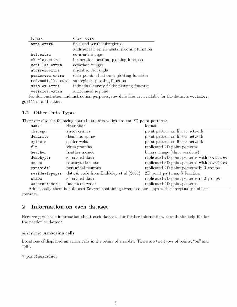
amacrine: Amacrine cells

Locations of displaced amacrine cells in the retina of a rabbit. There are two types of points, “on” and“off”.

> plot(amacrine)

3

amacrine

●

●

●

● ●

●

●

●●

●●

●

●

●

●

●

●●

●● ●

●●

●

●

●

●

●●

● ●

●●

●

●

●●●●

● ●

●

●●

●●

●●

●●

●

●●

●

●

●● ●●

●

●

●

●

●●

●

●

●

●

●

● ●

●

●

●●

●

●

●

●●

●

●

●●

●

●●

●

●

●

●

●●

●●

●

●

●

●

●

●

●●

●● ●

●●

●●

●

●●

●●

●

●

●●

●●

●

●

●●

●●

●

●

●

●

● ●

●●

●

●

●

●●

●

●

on

off

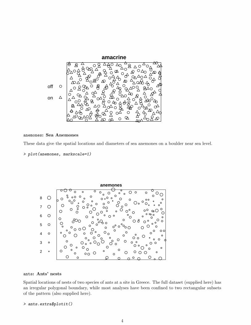
anemones: Sea Anemones

These data give the spatial locations and diameters of sea anemones on a boulder near sea level.

> plot(anemones, markscale=1)

anemones

● ●

● ●●

●●

●●

● ●●

●●

●●

●●

● ●●

●●●

● ● ●

● ●

●

●●

●

●

● ●

● ● ●

● ●

●●

●●

●

● ●

●●

●●

● ●

●●

● ●●● ●

●●

● ● ●

●

●●●

●● ●

●

●●

● ●

●●

● ●

●

●

●

● ●

●●

● ●

● ●

● ●

●● ●

● ●

●●

● ● ●

● ●● ●

● ●●

●●

●●

●

●●

●

●

●

● ●

● ●

●●

●●

●●

● ●

●●

●

●

● ●

● ● ●

●●

●●

●●

●●

●●

● ●

● ●

●●

● ●

●

● ●

● ●

●●

●●

● ●●

● ●●

● ●

●● ●

●●

● ●●

●●

●

●

●● ●

●

●●

●

●●●

● ●●

●

●●

●

● ● ●

● ●●

●●

●● ●

●

● ●● ●

●

●

●

●

●

●● ●

●

●

●

●

●

●

●

2

3

4

5

6

7

8

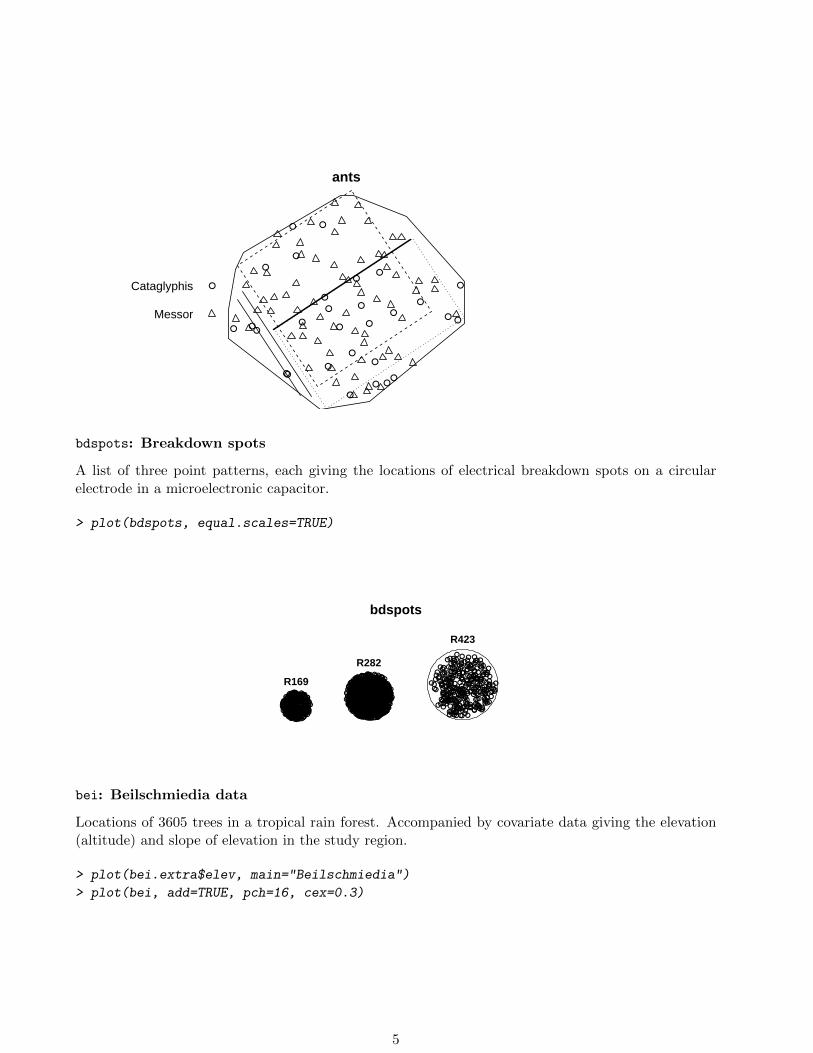
ants: Ants’ nests

Spatial locations of nests of two species of ants at a site in Greece. The full dataset (supplied here) hasan irregular polygonal boundary, while most analyses have been confined to two rectangular subsetsof the pattern (also supplied here).

> ants.extra$plotit()

4

ants

● ●

●

●

●●

●

● ●●

●

● ●●

●● ●

●● ●

●

●●

●●

●

● ●●

●

Messor

Cataglyphis

bdspots: Breakdown spots

A list of three point patterns, each giving the locations of electrical breakdown spots on a circularelectrode in a microelectronic capacitor.

> plot(bdspots, equal.scales=TRUE)

bdspots

R169●●●●●●●●●●●●●●●●●●●●●●●●●●●●●●●●●●●●●●●●●●●●●●●●●●●●●●●●●●●●●●●●●●●●●●●● ●●●●●●●●●●●●●●●●●●●●●●●●●●●●●●●●●●●●●●●●●●●●●●●●●●●●●●●●●●●●●●●●●●●●●●●●

●●●●●●●●●●●●●●●●●●●●●●●●●●●●●●●●●●●●●●●●●●●

●●●●●●●●●●●●●●●●●●●●●●●●●●●●●●●●●●●●●●●● ●●●●●●●●●●●●●●●●●●●●●●●●●●●●●●●

●●●●●●●●●●●●●●●●●●●●●●●●●●●●●●

●●●●●●●●●●●●●●●●●●●●●●

●

R282●●●●●●●●●●●●●●●●●●●●●●●● ●●●●●●●●●●●●●●●●●●●●●●●●●●●●●●●●●●●

●●●●●●●●●

●●●●●●●●●●●●●●●●●●●●●●●●●●

●●●●●●●●●●● ●●●●●●●●●●●●●●●●●●●●●●●●●●●●●●●●●●●●●●●●●●

●●●●●●●●●●●●●●●●●●●●●●

●●●●●●●●●●●●●●●●●●

●●●●●●●●●●●●●●●●●●●●●●●●●●●●●

●●●●●●●●●●●●●●●●●●●●●●●●●●●●●●●●●●●●●●●●●●●●●●●●●●●●●●●●

●●●●●●●●●●●●●●●●●●●●●●●●●●●●●●●●●●●●●●●

●●●●●●●●●●●●●●●●●●

●●●●●●●●●●●●●●●●●●●●●●●●●●●●●●

●●●●●●●●●●●●●●●●●●●●●●●●●●●●●●●●●●●●●●●

●●●●●●●●●●●●●●

●

●●●●●●●●●●●●●●●●●●●●●●●

●●●●●●●●●●●●●●●●●●●●●

●●●●●●●●●●●●●●●●●●●●●●●●●

●

●

●●

●●

●●

●●●●●●●●●●●●●●●●●●●●●●●●●●●●●●●●●●●●●●●●●●●●●●●●●●●

●●●●●●●●●●●●●●●●●●●●●●●●●●

●●●●●●●●

●●●●●●●●●●●●●●

●●● ●●●●●

●●●●●●●●●●●●●●●●●●●●●●●●●●●●●●●●●●●

●●●●●●●●●●●●●●●●●●●●●●●●●●●●●●●●●●●●●

●●●●●●●●●●●●●●●●●●●●●●●●●●●●●●●●

●●●●●●●●●●●●●●●●●●●●●●●●●●●●●●●●●

●●●●●●●●●●●●●

●●●●●●●●●●●●●●●●●●●●●●●●●●●●●●●●●●●●●●●●●●●●●●●●●

●●●●●●●●●●●●●●●●●●●●●●●●●●●●●●●●

●●●●●●●●●●●●●●●●●●●●●●●●●●●●●●●●●●●●●●●●●●●●●●●●●●●●●●●●●●●●●●●●●●●●●●●●●●●●●●●●●●●●●●●●●●●●●●

●●●●●●●●●●●●●●●●●●●●●●●●●●●●●●●●●●●

●●●●●●●●●●●●

R423

●●●●●●● ●

●●●●●●●●●●●●●●●●●

●● ●●●●●●

●●

●●●●●●●●●

●●●●●●●●●●●●●●● ●●●●●●

●●●●●

●

●●●● ●

●●●●●●●●●●●●●●●●

●●●●●●●●●

●●●●●●●

●●●●●●

●●●●●●●●●●●●●●●●●● ●● ●

●

●●● ●●●●●●●●●●●● ●

●●●●●●●●●●●●●●●●●●●●●●

●●●●●●●●●●●●●●●●●●●●●●●●●●●

●●●●●●●●●●●●●●●●●●●

●●●●●

●●●●●●●●●●●●

● ● ● ●●

●●●●●●●●●●●● ●●●●●

●●●●●●●●●

●●●●

●●●●●

●●●●●●●●●●●●●●

●● ●

●●

●●●●●● ●●●●●

●●●●●●●●

●●

●●

●● ●

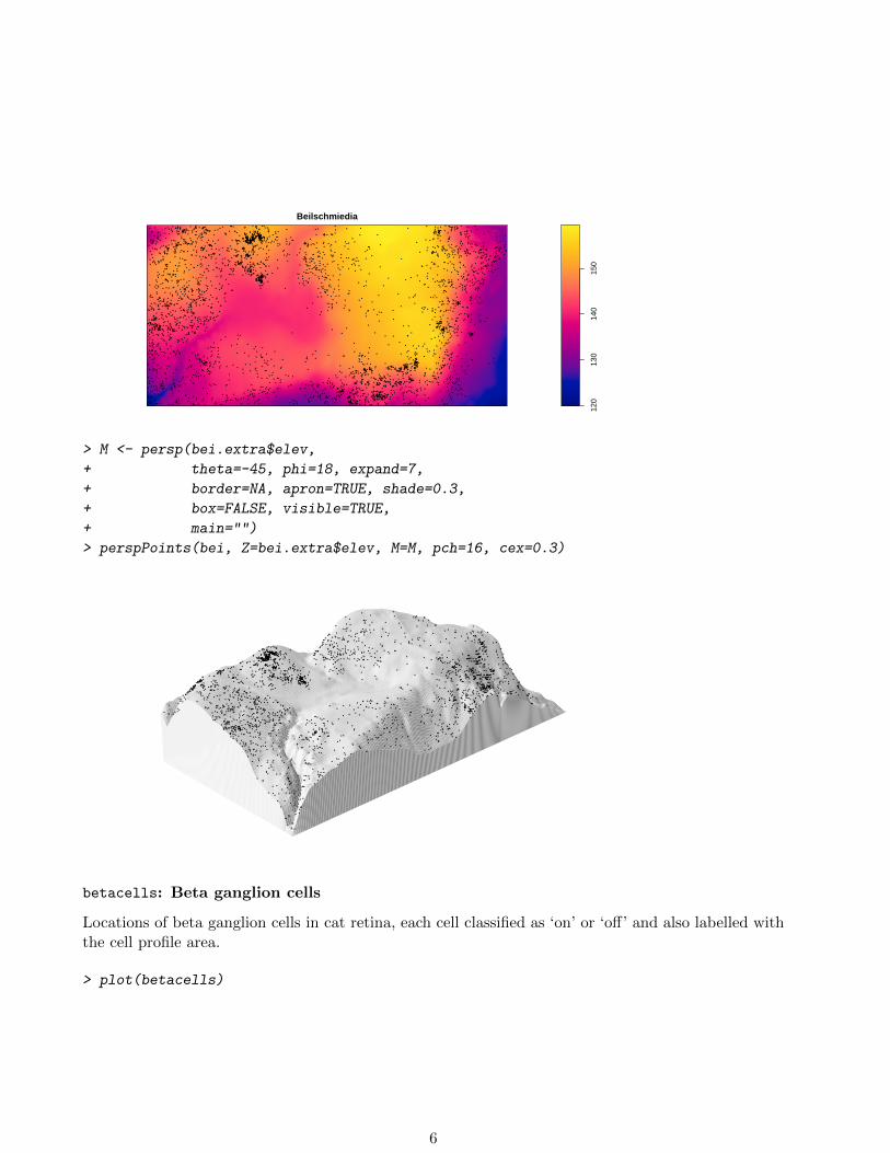
bei: Beilschmiedia data

Locations of 3605 trees in a tropical rain forest. Accompanied by covariate data giving the elevation(altitude) and slope of elevation in the study region.

> plot(bei.extra$elev, main="Beilschmiedia")

> plot(bei, add=TRUE, pch=16, cex=0.3)

5

Beilschmiedia

120

130

140

150

●

●●

●

●●

●

●

●

●

●

●

●

●

●

●

●

●

●

●

●

●

●

●

●

●

●

●

●

●

●

●

●

●

●

●

●

●

●

●

●

●●

●

●

●

●●

●

●

●

●

●

●

●

●

●

●●

●

●

●

●

●

●

●

●

●●

●

●

●

●

●

●

●●

●

●

●

●●

●

●

●

●

●

●

●●

●

●

●

●●

●

●

●

●

●

●

●●

●●

●

●

●

●

●

●

● ●

●

●

●

●

●

●

●

●

●

●

●

●

●

●

●

●

●

●

●

●

●

●

●

●

●

●

●

●

●

●

●

●

●

●

●

●

●●

●

●

●

●

●

●

●

●

●

●

●●

●

●

●

●

●

●

●

●

●

●

●

●

●

●

●

●

●

●

●

●

●

●

●

●●

●

●

●

●

●●

●

●●

●

●

●

●

●

●

●

●

●

● ●

●●

●●

●●

●●

●

●

●

●

●

●●

●

●

●

●

●●

●

●●

●

●

●

●

●

●

●●

●

●

●

●

●●● ●

●

●

● ●

●●

●

●●●

●●

●

●●●

●

●●

●

●

●

●●

●

●●●

●

●

●●

●

●

●●

●

●●●

●

●

●●

●

●

●●

●

●

●

●

●●●●●●●●

● ●

●

●

●

●●

●

●

●●

●

●

●

●

●

●●●●

●●

●

●●

●

●

●

●

●

●

●

●

●

●

●

●

●●

●●

●

●

●

●

●

●

●

●

●

●●

●

●

●

●●●

●● ●●

●

●

●

●●●

●

●

●

●

●

●

●

●●●

●

●●●

●

●

●

●

●

●●

●

●

●

●

●

●● ●

●

●

●

●

●

●

●

●●

●

●

● ●

●

●●

●

●

●

●

●

●

●

●

●

●

●●

●● ●

●

●

●

●

●

●

● ●●●●

●

●●

●●

●

●

●

● ●●

●

●●

●●

●● ●

●

●

● ●

●●

●

●

●

●●●

●●

●

●

●

●●●

●●●

●

●

● ●

●

●

●

●

●

● ●

●

● ●

●

● ●

●

●●●

●

●

●

●●

●●

●●

●●

●

●●●

●

●

●

●● ●●

●

●

●

●

●●

●

●

●

●

●

●

●

●

●

●●

●

● ●

●

●

●●

●

●

●

●

●●

●●

●

●

●

●●●

●

●

●

●

●

●●

●

●

●●

●●

●

●

●

●

●●● ●

●●

●

●●●

●

●

●

●●

●●●

● ●

●

●

●●●●

●

●

●

●●

●●●

●●●●

●

●

●

●

●

●

●

●

●

●

●

●

●●

● ●

●

●

●

●●●●●●●

●●●

●

●●●●●●

●●

● ● ●

●

●

●

●

●

●

●

●●

●

●

●

●

●

●

●●

●

●

●●●● ●

●

●

●●

● ●●●

●●●●

●●● ●

●

●

●●

●

●

●●●●●

●

●

●●

●

●

●

●

●●●

●●●

●●

●

●●

●●

●

●●●

●

●

●

●

●

● ●●●●

●

●

●● ●

●● ●

●●●

●●

●●●

●

●●●●●●●●●

●●

●

●

●

●●●

●●

●●

●●●

●●

●

●

●

●

●●●●●

●●

●●●●

●

●●

●●●●●●●●●●

●●

●

●●

●

●

●●

●

●

●

●

●

●●●

●●

●

●

●●

●

●●

●●●

●

●●

●

●

●

●●●

●

●

●

●

●

●●

● ●

●

●●

●

●

●

●

●

●●●

●

●●●

●●

●

●●

●

●●●●

●●

●

●

●●

●

●

●

●

●

●

●

●

●

●●●●

●●

●●●●●

●

●●

●●

●●

●●●

●

●

●

●

●

●●

●

●

●●

●

●● ●

●

●

●

●● ●

●●

●●●

●●

●

●

●

●

●

●

●

●

●

●●

● ●

●

●

●

●●

●

●● ●

●

●●

●

●

●

●

●●

●

●

●

●

●

●

●

●

●

●

●

●

●

●

●

●

●

●

●

●

●

●

●● ●

●

●

●

●

●

●

●

●

●

●●

●●

●●

●

●

●

●●

●●●

●●●

●

●

●

●●●●

●●

●

●● ●

●

●

●

●

●● ●

●

●●

●●

●

●

●●

●● ●

●

●

●●

●

●

●

●

●

●

●●

●

●●

●

●

●●●●

●

● ●●

●

●

●

●

●

●

●

●

●●

● ●●

●

●●

● ●

●

●

●

●● ●●

●

●

●

●●●

●●●

●

●

●

●

●

●

●

●

●

●

●

●●

●

●

●●●

●

●

●

●

●

●

●

●●

●

●

●

●

●

●

●●

●●●

●

●

●

●

● ●

●

●●

●●

●

●●

●

●

●●

●

●

●

●

●

●●

●

●

●

●

●

●

●

●

●

●

●

●

●

●

●

●

●

●

●

●● ●

●

●

●

●

●●

● ●

●

●

●●●

●

●●●

●●●

●● ●

●

●

●

●

●

●

● ●●

●●

●

●●

●

●●

●

●

●

●

●●

●●●

●

●

●●

●●

●●●●●

●●

●●● ●

●●●

●●●●●●●●●●●●

●●●●●

●●●●●●●●●

●

●

●●

●●

●●●●●●

●●

●

●

●●

●●

●●

●●●●

●

●● ●●

●

●●●●●●●●●●●●

●●●

●●●●

●

●

● ●

●●

●

●● ●

●

●●●

●

●

●

●

● ●●

●●●

●●●●

●●

●

●

●● ●●●

●●

●●

●

●●●●●

●●

● ●

●

●●

●

●●●●●●●●●

●●●●●●●

●●

●

●

●●

●●●

●●●

●●●●●●●●●●●●●●●

●●●●●●

●●

● ●●●●

●●

●

●●

●

●●●●●●

●

●●●●

●●●●●●

●●●●●●●

●

●

●

●

●●

●●●● ●

●●

●●●●●●●●

●●

●●

●

●●

●

●

●

●

●

●

●

●

●

● ●

●●●

●

●●

●●

●

●

●

●●●

●

●

●●

●

●

●

●

●●

● ●●

●●●

●

●●

●●

●●

●●

●

●●●

●

●

●

●

●

●

●

●

●

●●

● ●

●●●

●

●

●●

●

●●

●

●

●

●

●

●●● ●

●

●

●

●

●

●●

●

●

●

●●

●

●

●

●●

●

●●

●

●

●

●●

●

●●

●

●●

●

●●

●

●●

●

●

●●

●

●

●

●

●

● ●

●●

● ●

●

●●

●

●

●

●

●●

●

●

●●

●

●

● ●

●

●●

●●

●

●

● ●

●

●●

●●

●

●

●

● ●●

●●

●

●

●●

●●●

●

●●

●

●

●

●●

●

●

●

●

●

●

●

●●

●

●

●

●●

●

●

●

●

●

●

●

●

●●●

●

●

●●

●

●

●

●● ●●

●●

●

● ●●●●●

●

●●● ●

● ●●

●●

●

●●

●

●

●

●● ●

●

●

● ●

●●●●

●

●

●

●●●

●●

●

●●

●●

● ●

●●

●

● ●

●

●●

●

●

●●●●

●

●

●●

●●

●

● ●●

●

●●

●

●●

●●●

●

●

●

●

●●

●●

●

●

●

●

●●

●

●●

●●

●

●

●●●●

●●

●

●●

●

●●

●

●

●

● ●

●●●

●

●

●●

●

●

●

●

●

●●●

●

●

●●

●

●

●●●

●

●

●

●

●

●●

●

●

●

●

● ●

●●●

●●● ●●

●

● ● ●

●

●●

●●●

●

●

●

●

●● ●

●

●

●

●●

●

● ●●●●

●●

●

●●●●

●●

●●

●●

●●●

● ●

●●● ●

●

●

●

●●

●

●

●●● ●

●●

●

●

●●●●●

●

●

●

●

●

●

●

● ●

●●

●

●●

●

●

●●

●●●

●

●

●

●

●●●

●●

●

●

●

●

●

●

●●

●●●

●●

●●●

●

●

●

●

●

●

●●

●

●

●

●

●●

●

●●

●●

●●

●●

●

●●● ●

●

●

●

●

●●

●●●

●

●

●

●

●

●

●

●●

●

●

●

●●

●●

●

●

●

●

●

●

●

●● ●

●

●●

●

●

●

●

●

●●

●●

●●●●●

●●

●●●

●●

●

●

●

● ● ●

●

●●●

●

●

● ●

●

●

●

●●●

●

●

●●● ●●

●●●●●●●

●●●

●

●

●

●

●●

● ●

●

●●

●●

●

●

●

●

●

●●●

●

●

●●

●

●

●● ●

●

● ●

●

●

●●

●●●●●●●●

●●●

●

●●●

●

●●

●●●

●●

●●●

●

●

●

●

●

●●

●●

●

●

●●

● ●

●

●

●

●

●

●

●

●

●●

●

●●●

●

● ●

●

●

●

●●

●

●

●

●

●

●●

●

●●

●● ●

●

●

●● ●

●

● ●

●

●●

●

●

●

●

●

●●

●

●●

● ●

●●

●

●

●

●●

●●

●

●

●

●

●

●

●

●

●●●

●●●

●

●

●●

●●●●●●

●●

●●

●

●

●●

●●

●

●

●●

●

●

●●●

● ●

●

●

●

●●

●

●●●

●

●●

●

●

●

●

●

●

●●●

●

●

●

●

●●

● ●●

●

●

●●

●

●

●

●

●

●

●

●

●

●

●

●

●

●●

●

●

●

●●

●

●

●

●

●

●

●

●

●

●

●

●

●

●

●

●●

●

●●

●

●

●

●

●

●

●●

●

●

● ●●

●

●

●

●

●

●●

●●

●

●●

●●●

●

●

●

●

●

●

● ●

●●

●

●

● ●

●

●

●

●

●

●

●

●

●

●

●

●

●

●

●●

●

●

●●●●●

●

●

●●

●●●

●●

●●

●

●

●

●●●

●

●●●

●

●

●

●● ●●

●

●

●

●

●

●

●

●

●

●

●

●

●

●

●

●

●

●

●

●

●●●

●●●●●

●

●

●

●

●

●

●

●●

●

●

●

●

●

●

●

●

●

●●●●

●

●●

●

●●

●

● ●●●●

●● ●

●

●

●●●●●●●●●●●●●●●●●●●

●●●●●●

●

●

●

●●●

●●●

●●

●●●●●●

●

●

●●●●●

●●●●

●●

●●●●●

●● ●

●●●●●

●●

●

●

●

●

●

●

●

●●

●

●

●

●

● ● ●

●

●

●

●

●

●

●

●

●●

●

●

●

●

●

●

●●

●

●●

●

● ●

●

●

●●

●●

●●●●

●

●●

●●

●

●

●

●● ●

●

●

●●

●●

●

●●

●

●

●

●

●

●

●

●

●

●

●●

●●

●

●● ●

●

●

●●●●

●●●

●

●

●

●

●

●

●

●

●

●

●

●

● ● ●●

●●●

●

●

●

●

●

●

●

●

●●

●

●

●●

●

●

●

●

●●

●

●

●

●

●●

●●●

●

●

●

●

●●

●

● ●●●●

●

●

●

●

●

● ●●

●

●

●

●

●

●

● ●●●

●●●

●

●

●

●●●

●

●

●

●

●

●

●

●

●

●

●●

●

●

●

●

●

●

●

●

●

●

●

●●●●

●●●

●

●

●

●

●

●

●●●

●

●

●

●

●

●

●

●

●

●

● ●

●●

●

●●

●

●

●

●

●●●●●

●

●

●

●

●

● ●

●●

●

●

●

●●

●

●

●

●

●●

●●

●

●

●

●

●

●

●

●

●

●●

●

●

●

●

●

●

●

●

●

●●●

●

●

●

●

●

●

●●

●

●

●

●

●

●●

●

●

●

●

●

●●●

●

●

●●

●●

●

●

●

●

●●

●

●

●●

●

●

●

●

●

●

●

●●

●

●

●

●

●

●

●

●

●

●

●

●

●●

●

●

●

●●

●●

●

●

●

●

●●

●

●

●●

●

●

●

●●●●●

●

●

●●

●

●

●

●

●

●

●

●

●

●

●

● ●●●●

●

●

●

●

●

●

●

●

●●

●

●

●

●

●

●

●

●

●●

●

●●●

●●

●●

●

●

●● ●●●

●●

●

●

●

●

●●

●●

●

● ●

●

●

●

●

●

●

●

●

●

●

●

●

●

●●

●●

●

●

●

●

●

●

●

●●

●

●

●

●

●

●

●

●●●●

●

●

●●

●

●

●

●

●● ●

●●

●

●

●

●

●

●

●

●

●●●●●●

●●●

●●

●

●●

●

●●

●●

●●

●

●●

●

●

●●●

●

●

●

●

●●●

●●

●

●

●

●

● ●

●

●

●

●

●

●●

●

● ●

●

●

● ●

●

●

●

●●

●

●●

●

●●

●

●

●

●

●

●●●●●

●●●

●●

●●

●

●

●

●

●

●

●●

●

●

●

●●

●●

●●

●

●

●

●

●

●

●●●

●●

●●●

●●

●

●

●

●

●●●

●●●●●●●●●●●

●●

●●●

●

●

●●

●

●

●

●

●

●

●

●●

●

●

●

● ●

●

●

●

●

● ●

●●●● ●

●

●

●●

●

●

●

●●●

●

●

●

●●

●

●

●

●

●●

●

●

●

●●

●

●●

●

●

●

●

●●

●

●

●

●

●

●

●

●

●

●●●

●

●

●

●

●

● ●

●

●●

●

●

●

●

●

●

●

●●●●●●

●

●

●

●

●

●

●

●

●

●●

●

●●

●

●

●

●

●

●

●

●●

●

●

●

●

●

●

●

●

●

●

●

●

●● ●

●

●

●

●

●

●

●

●

●

●

●●

●●●

●

●

●●●

●

●

●

●

●

●

●

●

●

●

●

●

●

●

●

●

●

●

●

●●

●

●

●

●

●

●

●

●

●

●

●

●

●

●

●●●

●

●●

●

●

●

●

●

●

●

●

●

●

●

●

●

●

●

●

●

●

●

●

●●●

●

●●

●

●

●

●

●

●

●

●

●

●

●

●

●

●

●

●

●

●

●●

●

●●● ●

●

●

●

●

●

●

●

●

●● ●

●

●

●

●

●

●

●

●●●

●●

●

●

●

●

●

●

●

●

●●

●

●

●

●

●

●

●

●

●

●

●

●

> M <- persp(bei.extra$elev,

+ theta=-45, phi=18, expand=7,

+ border=NA, apron=TRUE, shade=0.3,

+ box=FALSE, visible=TRUE,

+ main="")

> perspPoints(bei, Z=bei.extra$elev, M=M, pch=16, cex=0.3)

●

●

●

●

●

●

●

●

●

●

●

●

●

●

●

●

●

●

●●

●●

●●

●●

●●

●

●●

●

●

● ●

●

●

● ●

●

●

●

●

●

● ●

●

●

●

●●

●

●

●

●

●

●●

●

●

●

●●

●

●

●

●

●

●

●

●

●

●●

●

●

●

●●

●

●

●

●●

●

●

●

●

●

●

●

●

●

●

●

●

●

●

●

●

●

●

●●

●●●

●●●

●●

●●

●●●

●

●

●

●●

●

●

●●

●

●

●

●

●

●

●●

●

●

●

●

●●

●

●

●●

● ●

●

●

●

●

●

●●

●

●

●

●

●

●●●

●

●●

●

●●

●

●●

●●●●

●

●

● ●

●

●

●

●

●●

● ●

●

●

●

●●●●●●●●

● ●

●

●●●

●

●●

●●

● ●●

●●

●

●

●

●

●●

●

●●

●

●●

●●

●

●

●●

●● ●

●

●

●●

●●●●

●

●●

●

●●● ●

●

●●

●

●

●●

●●●

●

●

●

●

●

●

●

●

●

●●●

●

●●●●

●

●●●

●

●

●

●

●

●●●

●●

●

●

●●

●● ●●

●●

●●

●●●

●

●●

●●

●●●●●

●●

●

●

●

●●●

●●

●●

●●●

●

●

●

●

●●

●●●●

●

●

●

●●●

●●

●●

●●●●●●●●●●

●●

●

●●

●

●●

●●

●

●

●

●

●●●

●

●●

●

●

●

●

●

●

●●●

●

●

●

●

●

●

●●●

●

●

●

●

●

●●

●

●

●

●●

●

●

●

●

●

●●●

●

●●●●●

●

●●

●

●●

●●

●●

●

●

●●●

●●

●

●

●

●●

●

●

●

●●

●

●

●●●●

●●

●

●

●●

●●

●●●

●

●

●

●

●

●●

●

●

●●●

●●●

●●

●

●●●

●●

●●

●

●●

●

●

●

●

●

●●

●

●

●

●●

●

●●

●●●

●

●

●

●

●

●

●

●

●

●

●

●

●

●●

●

●

●

●

●

●

●

●

●

●

●

●

●●

●

●

●

●

● ●

●

●

●

●●

●● ●●●●

●

● ●

●

● ●●

●

●

●●

●

●

●●

●●●●

●●

●●

●

● ●●

●

●●

●

●

●

●

●

●

●

●

●●

●●●

●

●

●●

●

●●

●

●●

●● ●

●●

●●●●

●

●

●●

●

●●

●

●

●

●●

●●

●●

●●

●●

●●

●●●

●

●●

●●

●

●●●●

●

●

●

●●●

●

●●

●

●

●

●●●

●●

●●

●●

●

●

●

●

●

●

●●

●

●

●●

●

●

●

●●●

●

●●

●

●

●

●

●

●

●●

●

●

●

●

● ●

●

● ●

● ●●●

●

●●

●

●

●●●

●●●

●● ●

●

●

●

●

●●

● ●●

● ● ●●

●

●

●●

●

●

●●●

●

●●

●●

●●●

●

●●●

●●●

●●●

●●

●●●●●●

●●●●●●●●●●

●●●●

●●●●●

●

●

●●●

●

●●●

●●●

●●

●

●●●

●●●

●

●● ●●

●●

●●●

●●

●●●●●●●●●●

●●●

●

●●●●

●

●

●●

●●

●

●

●

●

●

●●

●

●

● ●

●

●●●

●●

●

●●●

●

●●

●

●

●●

●●●

●● ● ●

●

●●●●●

●●

●●

●●●

●●●●●●●●

●●●●●●●●●●

●●

●

●●●●●

●●● ●●●●●

●●●●●●●●●●●●●●●●

●●

●●●●●●●

●●

●

●●●●●●● ●

●●●●●●●●●●●●●●●●●●

●

●●

●●●●●●●

●●●●●●

●●●●●●

●●

●

●●

●

●

●

●

●

●

●

●

●●

●●●

●

●●

●●

●

●

●

●●●●

●

●

●

●

●

●

●

● ●

●●●

●

●

●

●● ●●●

●

●●● ●

●

●

●

●

●

●

●

● ●

● ●●

●

●●●

●

●●

●●

●●

●

●●●

●

●

●

●

●

● ●

●

●

●●●

● ●

●

●

●●

● ●

●

●

● ●●

●●

●

● ●

●● ●

●

●

●●

●

●

● ●

●

●●

●●

●

●

● ●●

●●●●

●

●

● ●●

●●

● ●●

●

● ●●

●

● ●

●

●

●

● ●

● ●●

●

●

●●

●●

●

●

●

●●

●

●●

●

●

●●

● ● ●●●

●

●

●

●

●●

●

●●

●

●●

●

●●

●

●

●●

●●

●

● ●●●●

●●

●●●

● ●●

●

●●

●

●●

●●●

●●●

●●

● ●

●

●

●

●

●

●

● ●

●

●●

●

●

●

●●

●● ●

●●●

●

●

●●

●

●

●●●

●●●

●●

●●

●●●●

●

●

●

● ● ●●●

●

●

●

●

●

●●●

● ●

●●●●

●●

● ●●

●●

●●● ●

●●

●

●●

●

●

●

●●

●

●●●

●

●●

●● ●

●

●●●

● ●●●

●

●●

●

●●●

●●●

●

●

●

●● ●

●●

●

●

●

●●

●●

●

● ●

●●●

●

●●

●● ●

●●

●

●

●

●

●●

●

● ●

● ●

●●

●●

●

●●●

●●●

●●●●

●

●●

●

●

●

●

●

●

●●

●

●

●

● ●

●

●

●

●●●

●

●●

●●

●

●

●

●

●

●

●●

●●

●●

●●●

●●●

●

●

●● ●

●

● ●●●

●● ● ●

●●

●●●●

●

●

●●

●●

●

●

●

●

●

●

●

●

●

●

●

●●

●

●●

●●●

●

●●

●

●

●●●● ●●●●●●

●●●●●●

●

●

●● ●●●

●●

●●●

●

●

●

●

●●

●●

●

●

●●

● ●

●

● ●

●●

●

●

●●

●●

●●●●

●

●

●

●

●

●●

●

●●

●

●

●

●

●

●

●

●

●●

●

●

●

●

●

●

●

●

●

●

●●

● ●

●●

●●

●

●●●

●●

●

●

●

●●

●●

●●● ●●●

●

●●●

●●●

● ●●

●●

●●●

●

●●

●●

●

●●● ●

●

●● ●

●

●

●

●

●●●

●

●

●●●

●

●

●

●

●●

●●●

●

●

●●

●

●

●

●

●

●

●

●

●

●

●

●

●●

●

●

●

●●

●

●

●

●

●

●

●

●

●

●●

●●●

●

● ●

●

●

●

●●

●●

● ● ●

●

●

●

●●

●●

●

●●●

●

●

●

●

●

●

● ●

●●

●

●

●

●

●

●

●

●

●

●

●

●

●

●●

●●●

●

●

●●

●

●●●

●

●

●●●

●

●

●

●

●●

●

●

●

●

●

●

●

●

●

●

●

●●●

●●●●●

●

●●

●●

● ●●

●●

●●

●

●

●

●

●

●●●

●

●

●●

●

●●

●●

●●●●

●●●

●

●

●●

●●●●●●●●●●●●●●

●●

●●●●●●

●

●

●

●

●●●●● ●●

●●●●●●●

●

●● ●●●

●●●●●

●●

●●●●●●● ●

●●●●●

●●●

●

●

●

●

●

●

● ●

●

●

●

●

● ●

●

●

●

●●

●

●

●●

●

●

●

●

●

●

●●

●

●●

●

●

●

●

●

●●

●●

●●●

●

●

●

●

●

●

●

●

●

●●●

●

●

●

●

●●

●

●

●

●

●●

●●

●

●●

●

●● ●

●●

●

●●

●

●

●

●●●●

●●● ●

●

●

●

●

●

●●

●

●

●

●

●● ●●

●● ●

●

●

●

●

●

●

●

●●●

●

●●

●

●

●

●

●

●

●

●

●●

●●

●● ●

●

●

●

●

●

●

●

●●●●●

●

●

●

●

●

●●

●●

●

●

●

●

●

● ●●●

●

●

●

●

●

●

●●●

●

●

● ●

●

●

●

●

●

●

●

●

●

●

●

●

●

●●●●

●

●

●

●

●

●●

●

●●

●

●

●●

● ●

●● ●

●

●●

● ●

●

●●

●

●●

●

●

●

●

●

●

●●

●●

●●

●

●

●

●

●

●

●●

●

●

●

●●

●

●

●

●●●● ●

●

●

●

●

●

●

●

●

●

●●

● ●●●

●

●

●

●

●

●

●

●

●●

●

●

●

●

●

●

●

●

●●

●

●●●

●●●●

●

●

●

●●

●●

●●●

●

●

●

●●

●●●

●●

●

●

●

●

●

●

●

●

●

●

●

●●

●

●

●

●

●

●

●

●

●

●

●

●

●

●●

●

●

●

●●

●

●

●

●

●

●

●

●

●

●● ●

●

●

●

●

●

●

●

●

●

●

●●●

●●● ●

●

●

●

●

●

●

●●

●●

●●

●●

●

●●

●

●

●● ●

●

●

●

●

●

●●●●

●

●

●

●

●●

●

●

●

●●

●

●

●

● ●

●

●

●

●

●

●●

●

●●

●

●●

●

●

●

●

●

●●●●●

●

●●

●

●●

●

●●

●

●

●

●

●

●

●

●

●

●

●

●

●

●●●

●

●

●

●

●

●

●

●●

●

●

●

● ●

●

●

●

●

●

●

●

●

●

●

●

●●

●

●

●●●

●●

●

●●

●

●

●

●

●

●

●●●

●

●

●

●

●

●

●

●●

●

●

●

●●●

●

●

●●●

●

●

●

●

●

●

●

●

●

●

●

●

●

●

● ●

●

●

●

●

● ●

●

●

●

●

●

●

●

●

●

●

●

●●●

●

●●

●

●

●

●

●

●

●

●

●

●

●

●

●

●

●

●

●

●

●●●

●

●

●

●

●

●

●

●

●

●

●

●

●

●

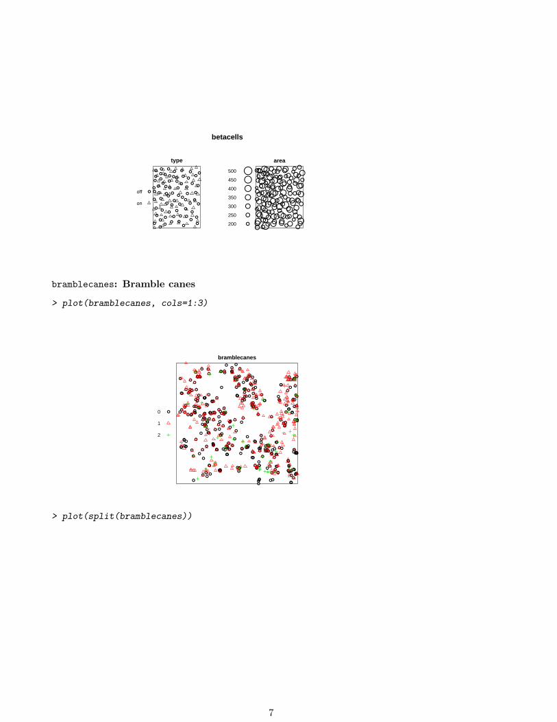
betacells: Beta ganglion cells

Locations of beta ganglion cells in cat retina, each cell classified as ‘on’ or ‘off’ and also labelled withthe cell profile area.

> plot(betacells)

6

betacells

type

●●● ●●

● ●● ●

● ●● ●●●● ●●● ●●

● ● ●● ●● ●●● ● ●● ●

● ●●● ●●●● ● ●●● ●

● ●●●●●

● ●●●● ●● ●●● ●●●● ●● ●

●

on

off

area

● ● ●● ●●● ● ●● ●●● ● ●●● ●● ●●●● ●● ●●● ●● ●● ●●● ●● ● ●●● ●●●● ●● ● ●● ●● ● ● ●●● ●●●● ● ●● ●● ●● ●● ● ●●●● ● ●● ● ●● ●● ● ●●●● ●● ●● ●●● ●● ●● ●●● ● ●● ●●● ●●● ●● ● ● ●●●●● ●●●●●● ●● ● ●● ● ● ● ●

●

●

●

●

●●●

200

250

300

350

400

450

500

bramblecanes: Bramble canes

> plot(bramblecanes, cols=1:3)

bramblecanes

●●●● ●●

●●

●●●●●

●●●●●

●●

●

●●●●●

●●●●

●

●●

●

●●

●

●●●

●

●●

●

●●●

●●●

●●

●

●

●●

●

●

●

●

● ●●

●●●●

●

● ●● ●●

●●

●●●●●

●●●●

●●●●●

●●

●

●●● ●

●●●●●●

●●●●●●●● ●●●

●

●

●

●●●●

●●

●●●

●

●

●

●

●●●●●

●

●●

●●

●

● ●● ●●

●●●●

●

● ●

●

●●●

●●

●

●●

●

●●

●●●

●●

●

●●●

●

●

●●

●●

●●

●●

●

●

●●

●●

●●●●

●

●●

●

●

●●

●●

●

●

●●

●

●

●

●

●●●

●●●●●

●

●

●●●

●●

●

●

●●●●

●●●●

●●●●●

●●●●●

●●

●

●●●

●●●●

●●●

●● ●●●

●

●●

●●●

●

●

●

●

●●

●

●●●

● ●

●

●●●●●

●●

●● ●

●●●

●

●

●●●

●●●

●

●

●●●

●●

●●●●

●

●

● ●●●

●

●

●●●

●●●●●

●

●

●

●

●

●●●● ●

●

●

●●

●

●

●●●●●

●●

●

●●●●

●

●

2

1

0

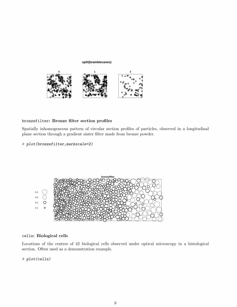
> plot(split(bramblecanes))

7

split(bramblecanes)

0

●●●● ●● ●●

●●●●●

●●●●●

●●●

●●●●●●●●●●

●●

●

●●●●●●

●

●●●

●●●●●●

●●

●

●●●

●

●●

●

●●●

●●●●

●

●●● ●●●●

●●●●●●●●●●●●●●

●●

●

●● ● ●● ●●●●●

●●● ●●●●● ●●●●

●

●

●●●●●●

●●●●●●

●

●●●●●

●

●●

●●

●

●●● ●●●●●●

●● ●

●

●●●

●●

●

●●●

●●

●●●●●

●

●●●

●●

●●

● ●●●

●●●

●

●●●●

●●●●●

●●

●

●

●●

●●●

●●●

●●

●

●●●●●●●●● ●●

●●●●●

●●

●●●●

●●●●

●●●●●

●●●●●

●●●●●●●●●●

●●●

●●●●●●

●●

●●●●

●●●

●●●

●●●

● ●

●

●●●●●

●●●●● ●●●●●●●●●●●

●

●●●

●●● ●●●●

●

●● ●●●

●●

●●●

●●●●●

●

●●

●●

●●●●●●

●●

●●

●

●●●●●●●

●●●●

●

●

1

●●

●●●●

●●● ●●●

●●●●●●●

●●●

●

●●● ●●● ●● ●●

●●●●

●●●●●●●●●●●●●●●●●●●●

●●

●●

● ●● ●●● ●●●●●●

● ●●●●●●●●●●

●●●●●●●●●

●●

●●●

●

●●

●●

●

●●

● ●

●●●

●●●● ●●●

●●

●

●●

●●

●●

●●●

●●●

●●

●●●

●

●●●●

●

●● ●●

●●●

●●●●●●●

●●●●

●●●

●● ●●●●●

●

●●●●●●

●●

●

●●●●●●

●●●

●●●●●●●●●●●

●

●●●

●●●●●●●●●

●

●●

●

●●●●

●●●●●

●●●●●●

●●●

●●●

●●●●●

●●●●●●●●●

●●●●

●●●

●●●●●

●●

●●

●●●●●●●●●●

●●●

●● ●●●●●●

●●●●

●●●●●●

●●●●●●

●●

●

●

●●●●●●

●●●●

●●●●●

●

●●

●●●●●●

●●●●

●●●

●●●●●●●●

●●●

●●●●●●●

●●

●●

●

●

●●

●

●●●●●

●●

●●●

●

●●●

●●

2

●●●●● ●●● ●

●● ●

●●●

●●●●●● ●

●●

●●●

●●●

●

●●

●

●●●

●●

●●●

●

●●●

●

●●

●●

●

●

●●●●

●●

●

● ●●

●●●●● ●●● ●

●●

●

●

●● ●

bronzefilter: Bronze filter section profiles

Spatially inhomogeneous pattern of circular section profiles of particles, observed in a longitudinalplane section through a gradient sinter filter made from bronze powder.

> plot(bronzefilter,markscale=2)

bronzefilter●● ● ●● ● ●●● ● ●● ●● ●● ● ●● ●● ● ●●●● ●● ● ●●● ●● ●● ● ●● ●●● ●●● ● ● ● ●● ●●●● ● ●●● ●●● ● ●●● ● ●● ●● ●● ● ●●● ● ●● ●● ● ●● ●●● ●●● ●● ●● ● ● ●●● ● ●●●● ●● ● ●●●● ● ●●● ● ● ●●● ●●● ●●●●●● ● ●● ● ●● ●● ●● ●●●● ● ●●● ●● ●● ●● ● ●●●●● ●●●● ●● ● ●●● ●● ● ●● ●● ● ● ●● ● ● ●● ● ● ●● ● ●●

● ● ●● ●● ● ●● ● ●● ●● ●●● ●● ●●● ●● ●● ● ●●●●● ● ●●● ●●● ● ●● ●●●●● ●● ● ● ●● ● ●● ● ●● ●● ●●●● ●● ● ●● ● ●● ● ●● ●●● ●● ●● ●● ●●● ●● ●●● ● ●●● ●●●● ●● ●● ● ●●●● ●● ●●● ● ●● ● ●● ●

● ●● ● ●● ● ● ●●● ● ●● ●●

● ●● ●●● ●● ●●● ● ●● ●●● ● ●●● ●

●● ● ●●● ●● ●● ● ●● ●●●●● ●●● ●●● ●● ●● ●●● ●● ●● ●● ●● ●●● ●●● ●● ●● ● ● ●● ●● ●● ●● ●●● ●● ● ●●● ● ●●● ● ● ●●● ●● ●●● ● ● ● ●●●●● ●●

● ● ●●●● ●● ● ● ●●● ●● ●●● ● ●● ● ●● ●● ● ●● ● ●● ● ● ●●● ●●●● ●●● ● ● ●●● ●● ●● ● ● ● ●●● ● ●● ●● ●

●●● ● ●● ● ●● ●● ●● ●●● ●● ●●● ●● ● ●●●● ●● ●● ● ●●●●● ●● ● ●●●● ●● ● ●● ●● ●●●● ●● ● ●●● ● ●●● ● ● ●● ● ● ●● ●● ● ●● ●● ● ● ●● ●● ●● ●● ● ● ●●

●●● ●● ● ● ●● ●●● ●●

● ●●

● ●● ●●●●● ●

●

●

●

0.1

0.2

0.3

0.4

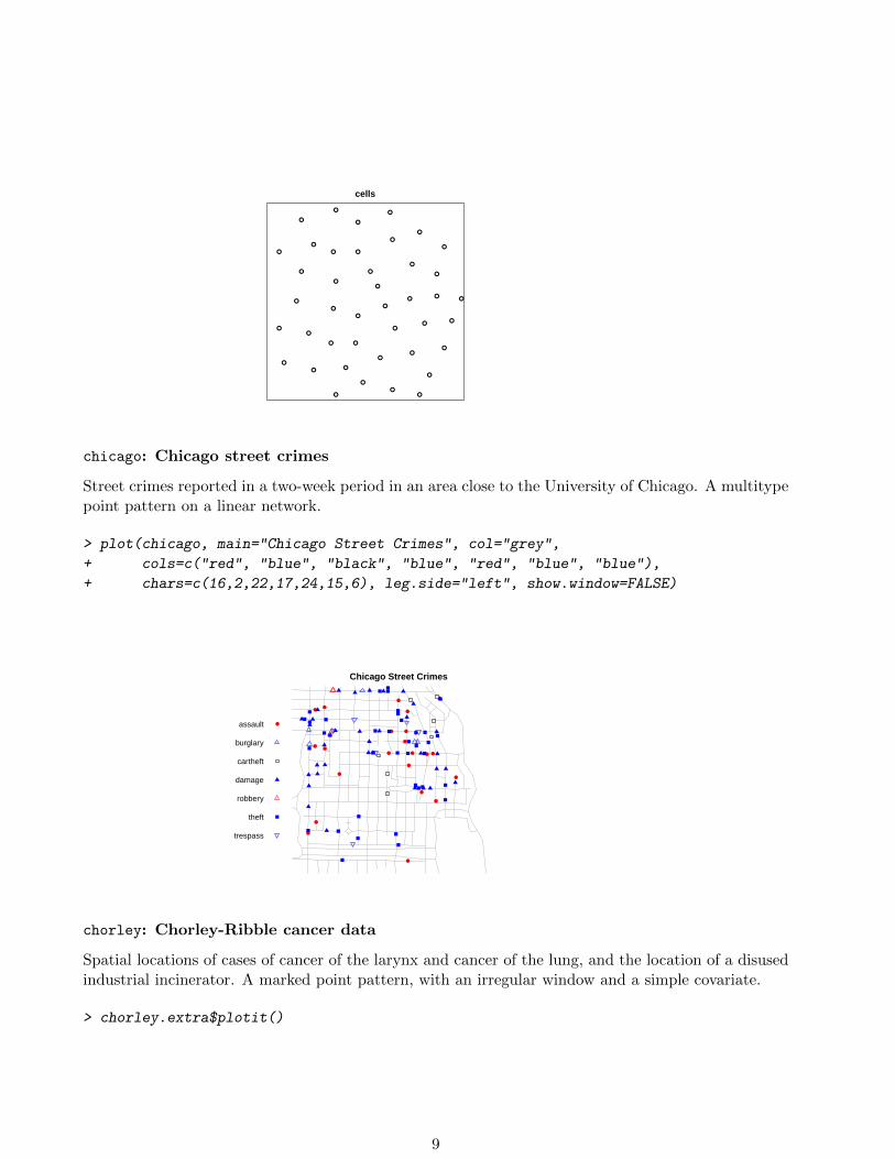
cells: Biological cells

Locations of the centres of 42 biological cells observed under optical microscopy in a histologicalsection. Often used as a demonstration example.

> plot(cells)

8

cells

●

●

●●

●

●

●●

●●

●●

● ●

●

●

●

●

●

●●

●

●●

●●

●

●

●

● ●

●

●

●

●●

●

●

●

●

●

●

chicago: Chicago street crimes

Street crimes reported in a two-week period in an area close to the University of Chicago. A multitypepoint pattern on a linear network.

> plot(chicago, main="Chicago Street Crimes", col="grey",

+ cols=c("red", "blue", "black", "blue", "red", "blue", "blue"),

+ chars=c(16,2,22,17,24,15,6), leg.side="left", show.window=FALSE)

Chicago Street Crimes

●

●●

●

● ●

●●

●● ● ● ●

●

●

●

●

●

●

●

●

●

trespass

theft

robbery

damage

cartheft

burglary

assault

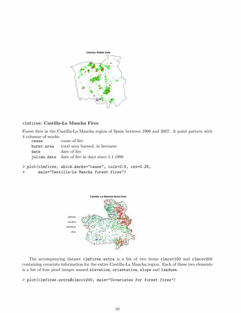
chorley: Chorley-Ribble cancer data

Spatial locations of cases of cancer of the larynx and cancer of the lung, and the location of a disusedindustrial incinerator. A marked point pattern, with an irregular window and a simple covariate.

> chorley.extra$plotit()

9

Chorley−Ribble Data

●

●

●

●

●

●

●

●

●

●

●

●

●

●

●

●

●

●

●

●

●

●

●

●

●

●

●

●

●

●

●

●

●

● ●

●

●

●

●●

●

●

●●

●

●

●

●

●

●●

●

●

●●●●●●

clmfires: Castilla-La Mancha Fires

Forest fires in the Castilla-La Mancha region of Spain between 1998 and 2007. A point pattern with4 columns of marks:

cause cause of fireburnt.area total area burned, in hectaresdate date of firejulian.date date of fire in days since 1.1.1998

> plot(clmfires, which.marks="cause", cols=2:5, cex=0.25,

+ main="Castilla-La Mancha forest fires")

Castilla−La Mancha forest fires

●

●

●

●

●

●

●

●

●

●

●

●●

●

●

●

●

●

●

●●

●

●

●

●

●●

●

●

●

●

●

●

●●

●

●

●

●

●

●

●

●

●

●

●

●

●

●

●

●

●

●●

●

●

●

●

●

●

●●

●

●

●

●

●●

●

●●

●

●

●

●

●

●

●

●

●

●

●

●

●

●●

●

●

●

●

●

●

●

●

●

●

●

●

●

●

●

●

●●

●

●

●

●

●

●

●

●

●

●

●

● ●

●

●

●●

●

●●

●

●

●

●●

●●

●

●

●

●

●

●

●

●

● ●●

●

●

●

●

●

●

●

●

●

●

●

●●●●●

●

●

●

●●

●

●

●

●

●

●

●

●

● ●

●

●

●

●

●

●

●

●

●

●

●

●

●

●

●

●

●

●

●

●

●

●

●

●

●

●

●●●

●

●

●

●

●

●

●

●

●

●

●

●

●

●

●

●●●

●

●

●

●

●

●

●●

● ●

●

●

●

●

●

●

●

●

●

●

●

●

●

●

●●

●

●

●

●

●

●

●

●

●

●

●

●

●

●●

●

●●

● ● ●

●

●

●

●

●

●

●

●

●

●

●

● ●

●●

●

●

●

●

●

●●

●

●

●

●

●

●

●●

●

●● ●

●

●

●

●

●

●●

●

●

●

●

●

●

●

●

●

● ●

●

●

●

●

●

●●

●

●

●

●●

●

●

●●

●

●

●

●

●

●

●

● ●

●

●

●

●

●

●

●

●

●

●

● ●

●

●

●●

●

●

●

●

●

●

●

●

●

●

●

●

●

●

●

●

●

●

●

●

●

●

●

●

●●●●

●

●

●

●

●

●

●

●

●

●

●

●

●

●

●

●

●

●

●

●

●

●

●

●

● ●

●

●

●

●

●

●

●

●

●

●

●

● ●

●●

●

●●

●

●

●

●

●●

●

●●●

●●●

●

●

●●

●●●●●

●

●

●

●

●

●

●

●

●

●

●

●

●●

●●

●

●

●●

●

●

●●

●

●

●

●●

●

●

●

●

●●

●

●

●

●

●

●

●

●●

● ●

●●●

●

●

●

●

●

●● ●

●

●

●

●

●

●

●

●

●

●●

●

●

●

●

●

●

●

●

●

●

●

●

●

●●

●

●

●

●

●

● ●

●

●

●

●

●●

●

●

●

●●

●

●●

●●

●

●

●

●

●

●

●

●

● ●

●●

●

●

●

●

●

●

●

●

●

●●

● ●

●

●

●

●

●

●

●

●

●●

●

●

●●

●

●●

●

●

●

●●

●

●

●

●●

●●

●

●●

●

●●

●

●●●

●

●

●

●

●

●

●

●●

●

●

●

●

●

●

●

●

●

●

●

●

●

●

●

●

●

●

●●

●

●

●

●

●

●

●

●

●●

●

●

●

●●

●

●

●

●

●

●

●

●

●

●

●

●

●

●

●

●

●

●

●

●

● ●

●

●

●●

●

●

●●

●

●

●

●

●

●

●

●

●

●

●

●

●

●●

●

●

●

●

●

●●

●

●

●

●

●

●

●

●

●

●

●

●

●

●

●

●

●

●

●

●

●●

●

●

●

●

●●

●

●

●

●

●

●

●

●

●

●

●

●●

●

●

●

●

●●●

●●

●

●

●

●

●

●

●

●

●

●

● ●●

●

●

●●

●

●●

●

● ●

●

●

●

●●

●

●

●

●

●

●

●

●

●

●

●

●

●

●

●

●

●

●

●

●

●

●

●

●

●

●

●

●

●

●

●

●

●

●

●●

●

●

●●

●

●

●

●

●

●

●

●

●

●

●

●

●

●

●

●

●

●

●

●

●

●

●

●

●

●

●

●

●●

●

●

●

●

●

●

●

●

●

●●

●

●

●

●

●

●

●

●

●

●

●

●

●

●

●

●

●

●

●

●

●

●

●

●

● ●

●

●

●

●

●●

●

●

●

●

●

●

●

●

●

●

●

●

●

●

●

●

●

●

●

●

●

●

●

●

●

●

●

●

●

●

●

●

●●

●

●

●

●

●

●

●

●

●

●

●

●

●●

●

●

●

●

●

●●

●

●

●

●

●

●

●

●

●

●●●

●●

●

●

●

●

●

●

●

●

●

●

●

●

●

●

●

●

●

●

●

●

●

●

●

●

●

●

●

●

●

●

●

●

●

●

●

●

●

●

●

●

●

●

●

●

●

●

●

●

●

●

●

●

●

●

●

●

●●

●

●

●

●

●

●

●

●

●

●●

●

●

●

●

●

●●

●

●

●

●

●

●

●

●

●

●

●

●●

●

●

●

●

●

●

●●

●

●

●

●

●

●

●●

●●

●

●

●

●

●

●

●

●

●

●

●

●

●

●

●

●

●●

●

● ●

●

●

●

●

●

●

●

●

●

●

●●

●

●

●

●

●

●

●

●

●

●

●

●

●

●

●●●

●

●

●

●

●

●

●

●

●

●

●

● ●

●

●

●

●

●

●

●

●

●

●

●●

● ●

●

●

●

●

●

●

●

●

●

●

●

●

●●

●

●

●

●

●

●

●

●

●

●

●

●

●

●

●

●●●

●

●

●

●

●

●

●

●

●

●

●

●

●

●

●

●

●

●

●

●

●

●

●

●

●

●

●

●●

●

●

●

●

●

●

●

●

●

●

●

●

●

●

●●

●

●

●

●

●

●

●

●

●●

●

●

●

●

●

●

other

intentional

accident

lightning

The accompanying dataset clmfires.extra is a list of two items clmcov100 and clmcov200

containing covariate information for the entire Castilla-La Mancha region. Each of these two elementsis a list of four pixel images named elevation, orientation, slope and landuse.

> plot(clmfires.extra$clmcov200, main="Covariates for forest fires")

10

Covariates for forest fires

elevation

500

1000

1500

2000

orientation

5010

020

030

0

slope

1020

3040

landuse

urba

nde

nsef

ores

tbu

sh

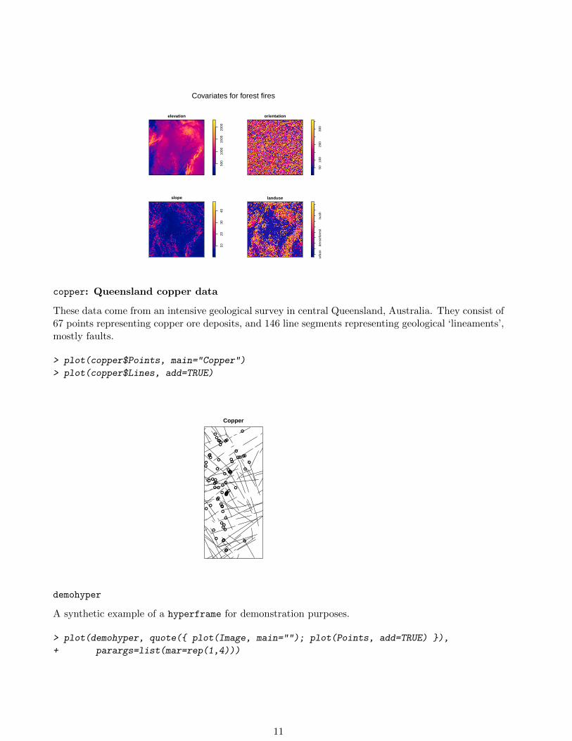
copper: Queensland copper data

These data come from an intensive geological survey in central Queensland, Australia. They consist of67 points representing copper ore deposits, and 146 line segments representing geological ‘lineaments’,mostly faults.

> plot(copper$Points, main="Copper")

> plot(copper$Lines, add=TRUE)

Copper

●●

●●●●

●●

●

●

●●●●●●●

●●

●

●

●●

●

●●●●

●

●

●●●

●●●

●●

●

●●

●●●●●

●●

●●

●●●

●

●

●

●●●

●●

●●●

●●

●

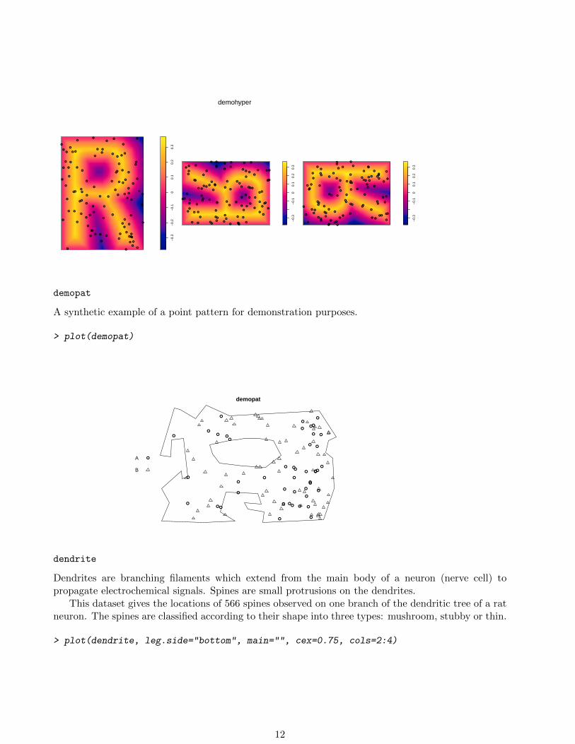
demohyper

A synthetic example of a hyperframe for demonstration purposes.

> plot(demohyper, quote({ plot(Image, main=""); plot(Points, add=TRUE) }),

+ parargs=list(mar=rep(1,4)))

11

demohyper

−0.

3−

0.2

−0.

10

0.1

0.2

0.3

●

●

●

●

●

●

●

●

●

●

●

●

●●

●

●

●

●

●●

●

●

●

●

●

●

●

●

●

●

●

●

●

●

●

●

●

●

●

●●

●

●

●

●

●

●

●

●

●

●

●

●

●

●

●

●

●

●

●

●

●

●

●

●

●

●

●

●●

●

●

●

●

●

●

●

●●

●

●

●

●

●

● ●

●

●

●●

●

●

●

●

●

●

●

●

●

●

●

●

●

●

−0.

3−

0.1

00.

10.

20.

3

●

●

●

●●

●●

●

●

●

●

●

●

●

●

●

●

●

● ●

●

●

●

●

●

●

●

●

●

●

●

● ●●

●

●

●

●

●●

●

●

●●

●

●

●

●

●

●

●

●

●

●

●●

●●

●

●

●

●

●

●

●

●

●

●

●

●

●

●

●

●●●

●

●

●

●

●

●

● ●

●

●●

●

●

●

●

●

● ●

●

●

●

●

●

●

●

●

●

●

−0.

3−

0.1

00.

10.

20.

3

●

●

●

●

●

●

●

●

●

●

●

●

●

●

●

●

●

●

●

●

●

●

●

●

●

●

●

●

●

●●

●

●

●

●

●

●

●

●

●

●

●

●

●

●

●

●

●

●

●

●

●

●

●

●

●

●

●

●

●

●

●

●

●

●

●

●

●

●

●

●

●

●

●

●

●

●

●

●

●

●

●

●

●

●

●

●

●

●●●

●

●

●

●

●

●

●●

●

●

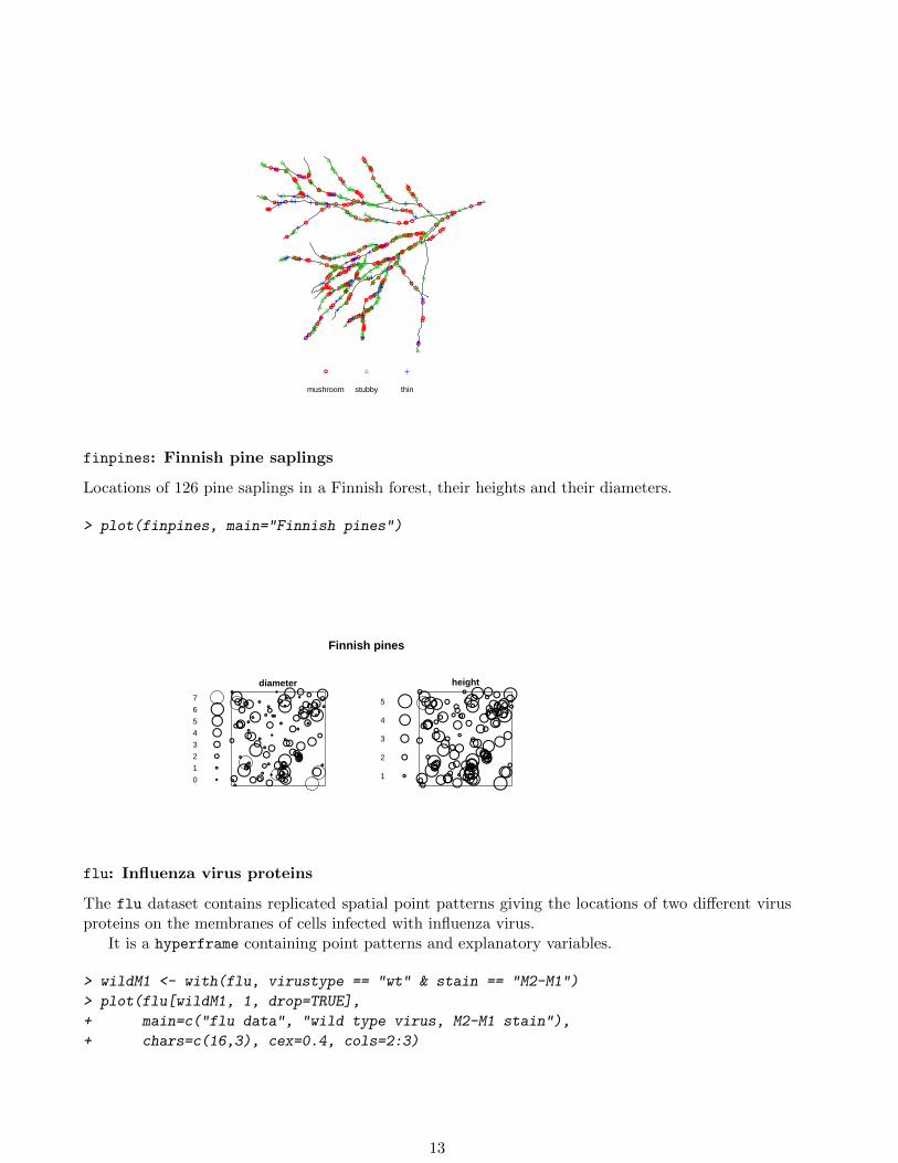
demopat

A synthetic example of a point pattern for demonstration purposes.

> plot(demopat)

demopat

●

●

●

●

●●

●

●

●●

●

●

●●

●

●

●

●

●

●●

●

●

●

●

●

●

●

●

●

●

●

●

●

●

●

●●

●

●

●

●

●

●

●

●

B

A

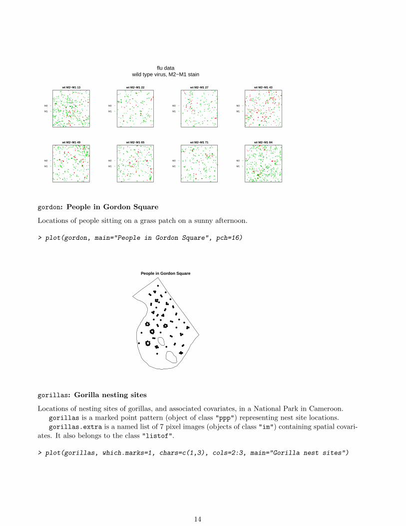
dendrite

Dendrites are branching filaments which extend from the main body of a neuron (nerve cell) topropagate electrochemical signals. Spines are small protrusions on the dendrites.

This dataset gives the locations of 566 spines observed on one branch of the dendritic tree of a ratneuron. The spines are classified according to their shape into three types: mushroom, stubby or thin.

> plot(dendrite, leg.side="bottom", main="", cex=0.75, cols=2:4)

12

●

●

●

●

●

●●

●

●

●

●

●

●

●

●

●

●

●

●

●

●

●

●

●

●

●

●

●

●

●

●

●

●

●

●

●

●

●

●

●

●

●

●

●

●

●

●

●

●

●

●

●

●

●

●

●

●

●

●

●

●

●

●

●

●

●

●

●

●

●

●

●

●

●

●

●

●

●

●

●

●

●

●

●

●

●●

●

●

●

●

●

●●

●

●

●

●

●

●

●

●

●●●

●

●

●

●

●

●

●

●

●

●

●

●

●

●

●●

●

● ●●

●

●

●

●

●

●

●

●

●

●

●

●

●

●

●● ●

●

●

●

●

●

●

●

●

●

●

●

●

●

●

●

●

●

● ●

●

●

●

●

●

●

●

●

●

●

●

●

●

●

●

●

●

●

●

●

●

●

●

●

●

●

●

●

●

●

●

●

●

●

●

●

●

●

●

●

●

●

●

●

●●

●

●

●

●

●

●

●

●

●

●

●

●

●

●

●

●

●

●

●

●

●

●

mushroom stubby thin

finpines: Finnish pine saplings

Locations of 126 pine saplings in a Finnish forest, their heights and their diameters.

> plot(finpines, main="Finnish pines")

Finnish pines

diameter

●

●

●

●●●●●●●

●●●

●●●●●

●

●

●

●●

●

●●

●

●

●

●

●●

●●●●●

●

●

●●●●

●

●

●

●

●

●

●

●

●●●●●●●●

●●

●●●●●

●

●

●●●●●●

●●●●

●●

●

●

●

●

●

●

●

●●●

●●●●● ● ●● ●●●

●●●●●●●●

●●●

●●

●

●●●●●●

●

●

●

●

●●●

0

1

2

3

4

5

6

7

height

●●

●

●●●●●●●

●●●●●●● ●

●

●

●

●●

●

●●

●

●

●

●

●

●●●●●●●

●

●

●●●●●

●

●

●

●

●●

●●●●●

●●●●●

●●●●●●●

●

●●●●●●●●●●●

●

●●

●●

●

●

●

●●

●

●●● ●●●●●●●●●●●● ●●●●●●●

●●●

●●

●

●●●●●●

●

●

●

●

●

1

2

3

4

5

flu: Influenza virus proteins

The flu dataset contains replicated spatial point patterns giving the locations of two different virusproteins on the membranes of cells infected with influenza virus.

It is a hyperframe containing point patterns and explanatory variables.

> wildM1 <- with(flu, virustype == "wt" & stain == "M2-M1")

> plot(flu[wildM1, 1, drop=TRUE],

+ main=c("flu data", "wild type virus, M2-M1 stain"),

+ chars=c(16,3), cex=0.4, cols=2:3)

13

flu datawild type virus, M2−M1 stain

wt M2−M1 13

●● ●●●●● ●●

●● ●●●

●

●●●●●●●● ●●● ●● ●●

●●● ● ●●●●●● ●● ● ●●●●●● ●●● ●

●

●●●●●●●

●●● ●● ●●● ●●●

●

●●● ●● ●●●●●●●●●

●●●●●

●●●● ●●●●

●● ●●●

●●●●●●

●●

●

●●

●

●

M1

M2

wt M2−M1 22

●

●

●●● ●●●●

●

●●

● ●● ●●●●

●●●●●●●

●

●●● ●

●●● ●

●●

●●●

●●●●● ●●

●

●●●●●●●●●●

●●●●

●●●

●

M1

M2

wt M2−M1 27

●●

● ●●●●●●●●●●

●●●●

●●●●●

●●●● ●● ●●

●● ●

●●●

●●● ●●●●●●

● ●● ● ●●

●●●●●●

●●●

●

●●●

●●●●●

●●

●

M1

M2

wt M2−M1 43

●

●●

●●●● ● ●● ●● ●●● ●●● ●●●●●●

●●●●

●● ●●●●

●●●●● ●● ●● ●●●●●● ●●● ●●● ●● ● ●● ●●●●● ●●●● ● ●

●● ●●●●●● ●●●●● ●●●●● ● ● ●● ● ●●●● ●●●● ●●

●●●●

● ●●● ●● ●●●●● ●●

●● ●

●●

●●● ● ● ●● ●●

●●●● ●● ●● ●●● ● ●●● ● ●●● ● ●●●● ●● ● ●● ● ●● ●●

● ●●● ●● ●●●● ●● ●● ●● ● ●● ●●

● ●●●● ●● ● ● ●●●●●●● ●●

●●●

●●● ●●●●●● ●

● ●

●● ●●● ●●●●●●

●●● ●● ● ●

●

M1

M2

wt M2−M1 49

●●

●●●

●●●●●

●●

●

●●●

●●

●●●●●

●●●● ●●●●●●●●

●

●●●● ● ●●●●●

●●●●●●●●●●●●● ● ●●●●● ● ●● ●● ● ●● ●●● ●

●

●● ●●●●● ●●●●●●●●●

●●● ●●

●●●● ●●●●● ● ●●●

●

●●●

●●● ●● ●● ●●●●●●●●

●●●●●● ●● ●● ● ●●● ●●●●●

●

M1

M2

wt M2−M1 65

●●

●● ●●

●●●●

●●

●●●● ●●●●●●

●

●●●●●●●●●●

●

●● ●●●● ●●●●

●●●●

●●●●●●●●

●●

●●● ● ●● ●●●●● ●●● ●● ●● ●● ●●●● ● ●●

●●●●●

●●

●●●●●● ●●●●●●●●●●

●

●

●

●●●●●

●

M1

M2

wt M2−M1 71

●●●● ●●● ●●●

●●●●●●●

●●

●●●

●●●●

●● ●

●●●● ●●● ●●●● ●

●●●●●

●●●●

●●●● ●● ●

●

M1

M2

wt M2−M1 84

●

●●●●●●●●●

●

●●●●●●●●●

●●●●

●

●●●●● ●●●●

●● ●●●● ●

●

●●● ●● ●●●● ●●●● ●●● ●●●●●●●

●●● ●●●

●

●●

●

●● ●●●

● ●●●●●●

●●

●● ●●●●● ●● ●● ●● ●●

●

M1

M2

gordon: People in Gordon Square

Locations of people sitting on a grass patch on a sunny afternoon.

> plot(gordon, main="People in Gordon Square", pch=16)

People in Gordon Square

●

●

●

●

●●

●

●

●●

●●

●

●

●●

●●

●●

●

●

●

●

●●●

●

●●●●

●

●●

●●

●●●

●

●●

●

●

●●●

●●●

●●

●

●●●●

●

● ●

●●●

●

●

●●●●●

●●

●

●

●

●●●

●

●●

●●

●

●●●

●

●●●●

●●●

●●

●

gorillas: Gorilla nesting sites

Locations of nesting sites of gorillas, and associated covariates, in a National Park in Cameroon.gorillas is a marked point pattern (object of class "ppp") representing nest site locations.gorillas.extra is a named list of 7 pixel images (objects of class "im") containing spatial covari-

ates. It also belongs to the class "listof".

> plot(gorillas, which.marks=1, chars=c(1,3), cols=2:3, main="Gorilla nest sites")

14

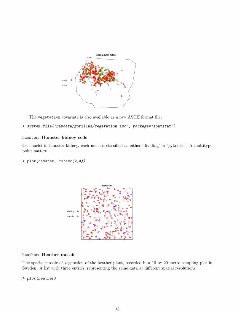
Gorilla nest sites

●

●

●

●●

●

●

●●

●

●●

●

●

●

●

●

●

●●

●

●

●●

●

●

●

●

●

●

●●

●

●

●

●

●

●

●

●

●

●

●

●●

●

●●●

●

●

●

●●●

●

●

●●

●●

●●

● ●

●●

●●●

●●●

●●

●

●

●

●●

●●● ●

●

●

●● ●●

●

●

●

●

●

●

●●

●

●●

●●

●

●

●

●●

● ●

●●

● ●

●

●

●

●

●

● ●●●

●●

●

●●

●●

●● ●

●

●

●

●

●

●

●

●

●

●

●

●

●

●

●

●

●

●

●

●

●

●

●

●

●

●

●

●

●

●

●

●

●

●●

●

●

●

●

●

●

●

●

●

●

●

●

●

●

● ●

●

●

●

●

●●

●

●

●●

●

●

●

●

●● ●

●

●

●

●

●

●●●

●

●●

●

●

●

●

●

●

●

● ●

●

●

●

●●

●●

●

●●

●

●

●●

●

●●

●●

●

●●●

●

●

●●

●●

●

●●●

●

●●

●

●

●

●●

●

●

●●

●

●

●

●

● ●

●

●

●

●

●

●

●

●●

●

●

●

●

●

●

●

●

●●

●

●

●●

●

● ●

●

●

●

●

●

●

●

●●

●

●

●

●

●

●

●

●

●

●

●● ●

●

●

●

●

●

●

●

●

●

●

●

●

●

●

●

●

●

●●

●

●

●

●

●

●

●

●

●

●

●

●

minor

major

The vegetation covariate is also available as a raw ASCII format file,

> system.file("rawdata/gorillas/vegetation.asc", package="spatstat")

hamster: Hamster kidney cells

Cell nuclei in hamster kidney, each nucleus classified as either ‘dividing’ or ‘pyknotic’. A multitypepoint pattern.

> plot(hamster, cols=c(2,4))

hamster

●

●

●

●

●

●

●●

●●

●●

●

●●●

● ●

●

●●

●

●

●

●

● ●

●

●●

●

●

●

●

●

●

●

●● ●

● ●

●●

●● ●

●

●●●

●●●

●●

●

●

●● ●

●

●●

●

● ●

●

●●

●

●

●●

●

●●

●●

● ●

●

●

●

●●

●

●

●

● ●

● ●

●●

●

●

●●

●●

●

●●

●

●

● ●

●●● ●

●

●●

● ●●

●●●

●●

●●

●

●● ●

●●

●

●

● ●

●● ●

● ●●

● ●●

●

●●

●

●

●

●

●

● ●

●

●

●● ●

●●

●

● ●

● ●●

●●

●

●●●●

●

●

●

●

●

●

●●

●

●● ●

●

●

●

● ●

●

●

● ●

●

●●

●

●●

● ●●●

●●●

●

●● ●

●

●

● ●●

●

●

●

● ●●

●

●

●

●

pyknotic

dividing

heather: Heather mosaic

The spatial mosaic of vegetation of the heather plant, recorded in a 10 by 20 metre sampling plot inSweden. A list with three entries, representing the same data at different spatial resolutions.

> plot(heather)

15

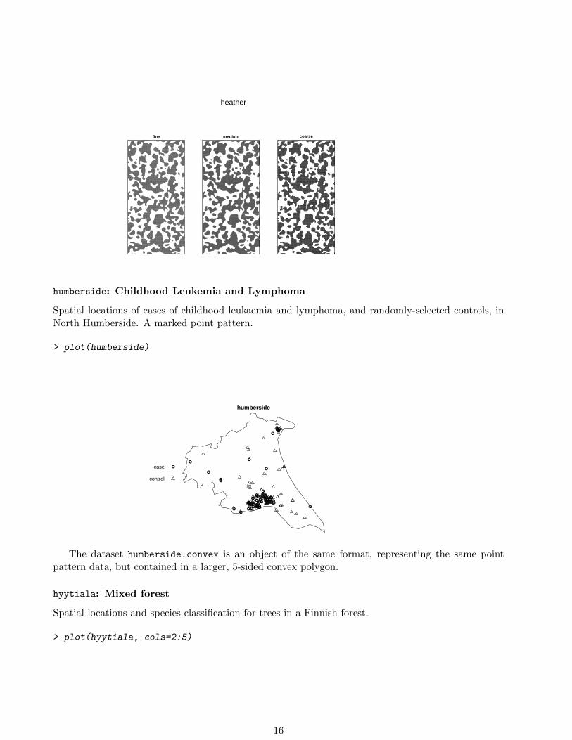
heather

fine medium coarse

humberside: Childhood Leukemia and Lymphoma

Spatial locations of cases of childhood leukaemia and lymphoma, and randomly-selected controls, inNorth Humberside. A marked point pattern.

> plot(humberside)

humberside

●

●●

●

●●

●

●●

●●

●

●

● ●

●

●

●

●

●

●

●

●●

●

●

●●

●

●

●

●●

●

●

●

●●

●

●

●

●

●●

●

●

●

●

●●

● ●

●

●

●

●

●

●●

●

●

●

●

control

case

The dataset humberside.convex is an object of the same format, representing the same pointpattern data, but contained in a larger, 5-sided convex polygon.

hyytiala: Mixed forest

Spatial locations and species classification for trees in a Finnish forest.

> plot(hyytiala, cols=2:5)

16

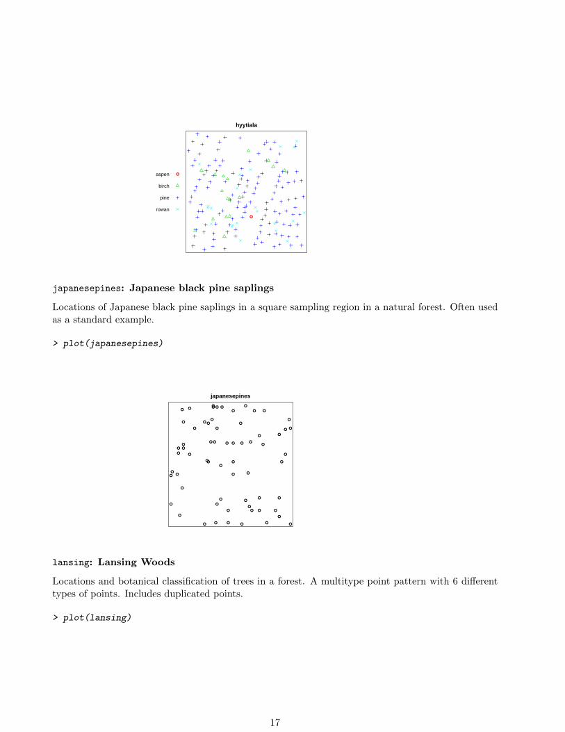
hyytiala

●

●

rowan

pine

birch

aspen

japanesepines: Japanese black pine saplings

Locations of Japanese black pine saplings in a square sampling region in a natural forest. Often usedas a standard example.

> plot(japanesepines)

japanesepines

●

● ●

●

● ●

●

● ●

●

●

●

●

●

●

●

●

●● ●

●

●● ● ●

●

● ●

●

●

●●

●

● ●

●

● ● ● ● ● ●●

● ●

● ●

●●

● ●

●

● ●

●

●

●

●

● ●

●● ● ● ●

lansing: Lansing Woods

Locations and botanical classification of trees in a forest. A multitype point pattern with 6 differenttypes of points. Includes duplicated points.

> plot(lansing)

17

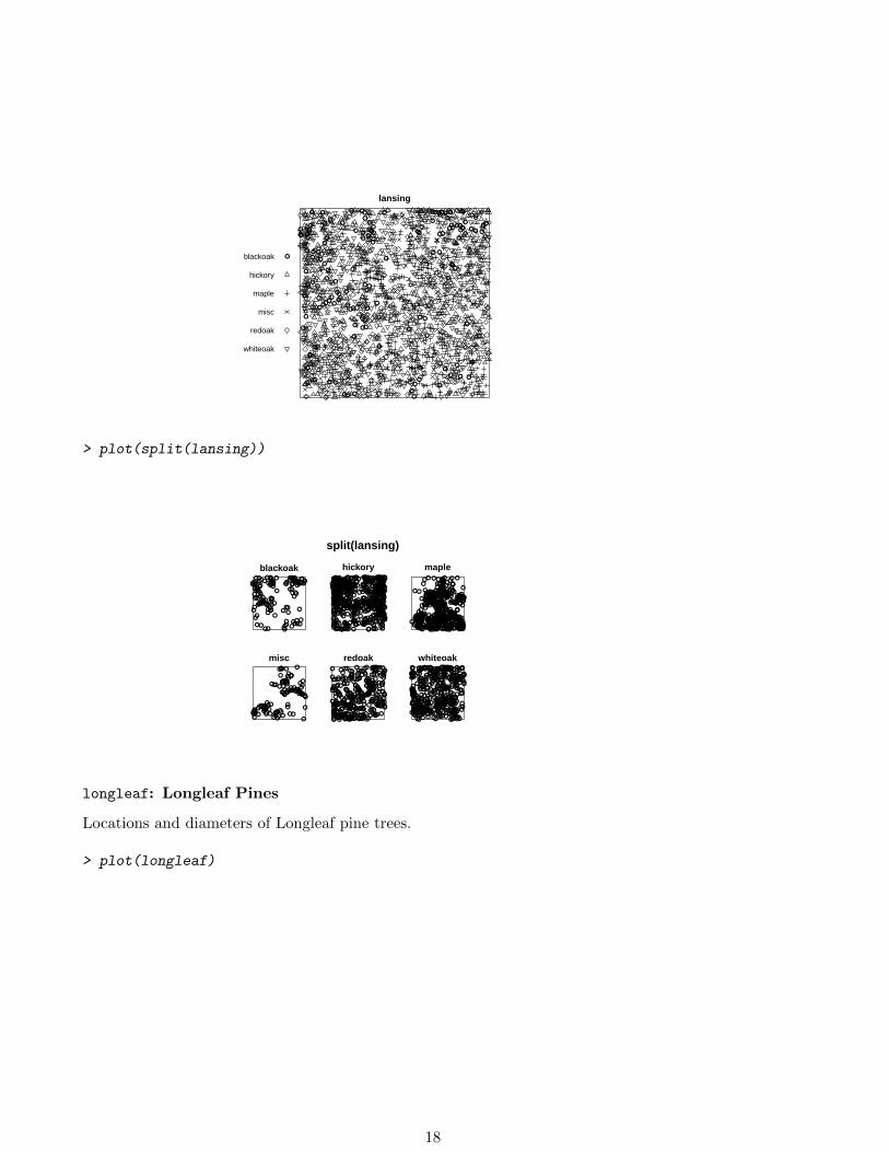
lansing

●

●

●

●

●

●●●

● ●●

●

●

●

●

●

● ●●

●

●●

●●●

●●●

●●● ●

●● ●

●●

●

● ●●

●●●

●●

●

●

●

●

●

●

●●●

●

●●

●●

●●●

●●●

●● ●●●●

●●

●●

●

●

●

●●

●●

●

●

●

●

●

●

●●

●

●

●●

●●

●●●●●●●

●●●●●●

●

●

●

●

●●●

●●

●

● ● ●

●

●

●● ●

●

● ●

●●

●●

●

whiteoak

redoak

misc

maple

hickory

blackoak

> plot(split(lansing))

split(lansing)

blackoak

●

●●

●●

●●●●●●●●

●●●●●●●●●●●●●●●●●

●●●● ●

●●

●

●●●●●●●●●

●

●

●

●●

●●●●●●● ●●●●

●●●●●●●●●●●

●●● ●

●

●●●●●

●●

●●

●●●●

●●●

●●●●●●●●●●●●●●●●

●●

●●●●

●●●

●●●●

●

●●●●●●●●●●

hickory

●●●●●

●●●●●●●●●

●●

●●●●●●●●●

●●●●●●●●

●●●●●●●●●●●●●●●●●●●●●●●●●●●●●●●

●●●●●●●●●●●

●●●●●●●●●●●●●●●●●●●●●●●●●●●●●●●●●●●●●●●●●●

●●●●●●●●●●●●●●●●●●●●●●●●●●●●●●●●●●●●●●●●●●

●●

●

●●●● ●●●●●●●●●●●●●●

●●●●●●●●

●●●●●●●●●

●●●●●●●●●●●●●●●●●

●●●● ●●●

●●●●●●●

●●●●●●●●●●●●

●●●●

●●●●●●●

●●

●●●●

●●●●●

●●●●●●●●●●

●●●● ●●●●●

●●●

●●●

●●●●●●●●●●●●●●●●●

●●●●●●●●●●●●●●●●●●●●●●●●●●●●●●●●●●●

●

●

●●●● ●●●●●●● ●●●●●●

● ●●●●

●

●●●●●●●●●●●

●●●●●●●

●●●●

●●●●

●●●

●●●●●●

●●●●●●●●●● ●●

●●●●●●●●●●

●●●●●●●●●●●●●●

●● ●●●●●●● ●●●●●●●●

●●●

●●●●●●●●

●●●●●●●●●●●●●●●●●●●●

●●●●●●●●●●●●●●

●●●●●●●●●●●

●●●●●●●●●

●●●●●●●●●●●●●●●●●●●●●

●●●●●●●

●●●●

●●●●●

●●●

●●●●

●●●●●●●●●●●●●●●●●●●

●●●●●●●●●●●●●●●●●

●

●●●●●●●●●●●

●●●●●●● ●●●●●●●●

●●●●●●●●●●●●●●●●●

●●●●●●●●●●●●●●●●●●●●●●●

●●●●●●●●●●●

●●●●●●●●●●●●●●●●

●

●●●●●●●●●

●●

maple

●●●●●●●

● ●●●●●●●●●●●●●●●●●●●

●

●

●●

● ●

●●●●

●●●

●●●●

●●●

●●

●●●●●●●●●●●●

●●●●

●●●●●●●●●

●●●●●●●●●●●●●●●●●●●

●●●●

●●●●●●●●●●●●●●

●

●●● ●●●●●●●●●●●

●●●●●●●●●●●●

●●●●●●●●●●●●●●●●

●●●●●●●●●●●●●

●●●●●●

●●●●●●●

●●●●

●●●●●●●●●

●●●●●●●●●●●●●

●●●●

●●●●●●●●●●●●

●●●●

●●●●●●●●●●●●●●●●●

●●●●●●●●●●●●

●●●

●●●●●●●●●

●●●●●●●●●●●●●●●●

●●●●●●●●●●●●●●●●●●●●

●●●●●●●●●●●●●

●●●●●●●●●●●●●●● ●●●●●●●●●●●●●●●●●●●

●●●●● ●●

●●●●●●●●●●●●●●●

●●●●●●

●●

●●●●●

●

●●●●●

●●●●●●●●●

●●●●●●●●●●● ●●

●●●

●●●●●●●●●●●●●

●●●●● ●●

●●●●●●●● ●●●●●●●●●●●●●●●

●●●●●●●●●●●●●●●●●●●●●●●●●●●●●

●●●●●●●●●●●●

●●●●●●●●●●

●

●

●

●

misc

●●●●●●

●●●●●

●

●●●●●●●●●●●

●●●●

●●●

●●

●●●●

●

●

●●●

●●

●●●●●

●●● ●

●●

●●●●●●●

●●●●●●●●●

●●●

● ●

●●●

●● ●●●●●●●

●●

●

●●●● ●●●

●●●●●●●

●

redoak

●● ●●●●●●●●

●●●●●●●●●●

●●●

●●●●●●

●●●●●●●●●●●

●●●●●●●●

●● ●●●

●●●●●

●●●

●

●●●●●●

●●●●●●●

●●●●

●●●

●●●●

●●●●●●●●●●●

●●● ●

●●●●●●●●●●●●●

●●●●●●●●●●●●●

●●●●●●

●●●●●●●●●●●●●● ●●●

●●● ●●●●●●●●● ●●●

●

●●●●●

●●●●

●●●●

●●●●●●

●●●●

●●

●●●●●●

●●●●●●●●●●●●●●●●●●

●●●●●●●

●●●●●●●●●●●●●

●●●●●●●

●●●

●●●●●●●●●●●●●

●●●●●

●●●●●●●●●●●●●

●●●●

●●●● ●●●●●

●●●●

●

●●●●●● ●

●●●●●●●●●●●●●●●●

●● ●●●

●●●●

●●●●●●●●

●●●●●●●●●

●●●

whiteoak

●●

●●●●●●●

●●●●●●●●●●●●●

●●●●●●●●●●●●●●●●●

●●●●●●●●●●●●●●●●●●●●●

●●

●●●●●●●●●●●●●●● ●●

●●●

●●●●●●●●●

●●●●●● ●●●

●●

●●●●●●

●●●●●

●●●●● ●

●●●●

●●●●●●●●●●●●●●●●●●●●

●●●●●●●

●●● ●●●●●

●●●●

●●● ● ●●●●

●●●●●●●

●●●

●●●●●●

●●●●●●●●

●●●● ●●●●

●●●●●●●●●

●●●●●●●●●

●●●●●●

●

●●●●●●●

●●●●●●

●●●

●●●

●●●●●●●●

●●●●●●● ●●

●●●●●●●●●

●●●●●●●●●●●●●

●●●●●●●●●

●●●●●●●

●●●●●●●●●

●●●●●●●●

●●●●●●●●●●●●●●

●●●● ●●●●●●●●

●●●●●●●●●●●●●●

●● ●●●●●

●●●●

●

●●●●●●● ●●●●●●●●●

●●●●●●●●●

●●

●●● ●●●●●●●●●●●●●●●●

●●●

●● ●●●

●●●●●●●●●●●●●●●

●●

●●●●●

●●

longleaf: Longleaf Pines

Locations and diameters of Longleaf pine trees.

> plot(longleaf)

18

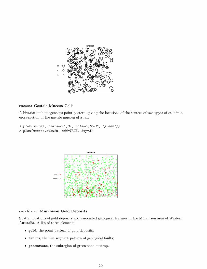
longleaf

●●●

●

●●●●

●●●●

●

●

●

●●●

●

●●●●●●

●●●

●●

●● ●●●● ●● ●●

●

●

●

●●●●● ●●●

●●●●●

●●●●

●

●

●●

●●

●●●

●●●●●

●●●●●

●●●●●● ● ●● ●●

●

●

●●

●●

●

●●

●●●

●●●

●

●●●

●●●

●●

●●●

●●●

●●

●●

●

●●

●●

●●

●

●●●

●●●

●

●

●●

●●●●●

●●

●

●

●●

●

●●

●

●●●

●●

●

●

●

●●●

●

●

●

●

●

●●

●●

●

●

●

●●●●

●●●●●

●●●●●

●● ● ●

●●●

●

●●●

●●●●●

●●●●

●●●●

●●

●

●

●

●●

●●●

●●●●

●●●

●● ●●●

●●●

●●●

●

●●

●●

●●

●●

●●

●

●

●●

●●●●●

●●

●

●●

●●

●●●●●

●

●●

●

●

●●

●●

●●

●

●●●●●●●●

●●●

●

●●

●

●

●●●

●

●●

●

●●

●●

●●●

●

●

●

●

●●●

●

●

●●

●

●

●●●

●●

●

●

●

● ●● ●

●

●●●

●●●●●●●

●

●

●

●●●●

●

●●●●

●

●

●●

●●●

●●

●●●

●●

●

●●●

●●●●

●●●

●●

●

●

●

●●●

●●●●

●●

●

●●

●●● ●●●●●●

●●

●

●●

●

●●●●●

●

●

●●

●●●●

●

●●

●

●

●

●●●

●●

●●

●

●

●●

●●●●

●

●●

●●●●●

●●

●

●●●

●●●

●

●

●

●

●●●●●●

●●

●

●●●●●

●●●●●

● ●●●

●●

● ●●●●

●●●●●●●

●

●●

●●●●●● ●

● ● ●●●●●●●

●

●

●

●

●●

● ● ●●●

●

●●●●●

●

●●

●●●●

●

●●●●

●●●

●● ●

●●

●

●●●●●●

●

●●

●

●

●

●

20

40

60

mucosa: Gastric Mucosa Cells

A bivariate inhomogeneous point pattern, giving the locations of the centres of two types of cells in across-section of the gastric mucosa of a rat.

> plot(mucosa, chars=c(1,3), cols=c("red", "green"))

> plot(mucosa.subwin, add=TRUE, lty=3)

mucosa

●● ●

●● ●

● ●

●

●●

●

●

●

●

●

●●●

●●

●●

●● ●

●● ●

●●

●●

●

●

●●

●

●

●

●

●

●●

●

●●●

●

●●

●●●●

● ●●● ●

●●

●

●●

● ●

●

●

●

●

●

●

●●●

●●

●

●

●

●

●●

●●

●

●●

●

other

ECL

murchison: Murchison Gold Deposits

Spatial locations of gold deposits and associated geological features in the Murchison area of WesternAustralia. A list of three elements:

� gold, the point pattern of gold deposits;

� faults, the line segment pattern of geological faults;

� greenstone, the subregion of greenstone outcrop.

19

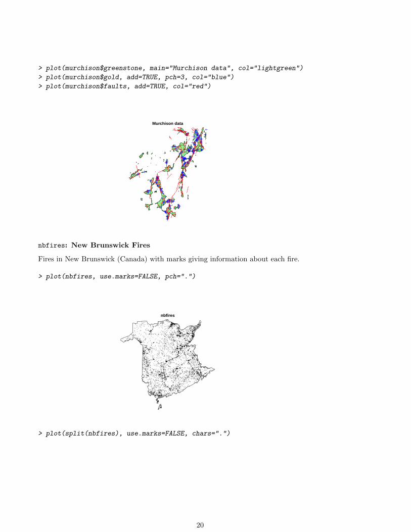
> plot(murchison$greenstone, main="Murchison data", col="lightgreen")

> plot(murchison$gold, add=TRUE, pch=3, col="blue")

> plot(murchison$faults, add=TRUE, col="red")

Murchison data

nbfires: New Brunswick Fires

Fires in New Brunswick (Canada) with marks giving information about each fire.

> plot(nbfires, use.marks=FALSE, pch=".")

nbfires

> plot(split(nbfires), use.marks=FALSE, chars=".")

20

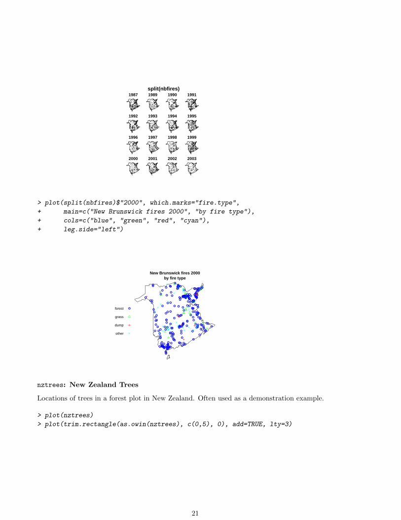
split(nbfires) 1987 1989 1990 1991

1992 1993 1994 1995

1996 1997 1998 1999

2000 2001 2002 2003

> plot(split(nbfires)$"2000", which.marks="fire.type",

+ main=c("New Brunswick fires 2000", "by fire type"),

+ cols=c("blue", "green", "red", "cyan"),

+ leg.side="left")

New Brunswick fires 2000by fire type

●

●●

●

●●

●

●●

●

●

●

●

●●

●●

●

●

●

●

●●

●

●●

●●

●

●

●

●●● ●

●

●●

●

●●

●

●

●●

●

●●

●

●

● ●●●

●

●●

●

● ● ●●

●

●

●● ●

●●

●

● ●●●●●

●

●●●●●●

●

●●●●

●●

●

●●●

●

●● ●●

●

●

●

●

●

●●● ●●●●

●

●

●

●●

●

●

●●

●●

● ●

●

●

●●●

●

●●

●

●

●

●

●

●●

●●●

● ●

●

●

●

●

●●●

●

●

●

●

●●

●

●●

● ●●●●

●

●●

●

●

●

●

●

●

●

●●

●●●

●●

●●●

●

●

●

●●

●●●

●

●●

●● ●●

●

●

●●

●

●

●

●

●●

●

●

●

●

●●

●●

●

●

●

● ●

●

●

●●●

●

●

●●

●

●

●

●●

●

●

●

●

●

●

●

●●

●●

other

dump

grass

forest

nztrees: New Zealand Trees

Locations of trees in a forest plot in New Zealand. Often used as a demonstration example.

> plot(nztrees)

> plot(trim.rectangle(as.owin(nztrees), c(0,5), 0), add=TRUE, lty=3)

21

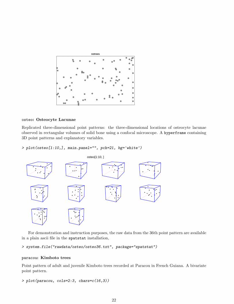
nztrees

●

●

●

●

●

●

●

●

●

●

●●

●

●

●

●

●

●●

●

●

●

●●●

●

●●

●

●

●

●

●

●●

●

●

●

●

●

●

●

●●

●

●

●

●

●

●●

●

●

●

●

●

●

●

●

●●

●

●●

●

●

●

●

●

●

●

●

●

●

●

●●

●

●

●

●

●

●

●

●

●

osteo: Osteocyte Lacunae

Replicated three-dimensional point patterns: the three-dimensional locations of osteocyte lacunaeobserved in rectangular volumes of solid bone using a confocal microscope. A hyperframe containing3D point patterns and explanatory variables.

> plot(osteo[1:10,], main.panel="", pch=21, bg='white')

osteo[1:10, ]

●

●

●

●

●

●

●

●

●

●

●

●

●

●

●

●

●

●

●

●

●

●

●

●

●

●

●

●

●

●

●

●

●●

●

●

●

●

●

●

●

●

●

●

●

●

●

●

●

●

●

●

●

●

●

●

●

●

●

●

● ●

●

●

●

●

●

●

●

●

●

●

●

●

●

●

●

●

●

●

●

●

●●

●●

●

●

●

●

●

●

●

●

●

●

●

●

●

●

●

● ●

●

●●

●

●

●

●

●

●

●

●

●

●

●

●

●●

●

●

●

●

●

●

●

●

●

●

●

●

●

●

●

●

●

●

For demonstration and instruction purposes, the raw data from the 36th point pattern are availablein a plain ascii file in the spatstat installation,

> system.file("rawdata/osteo/osteo36.txt", package="spatstat")

paracou: Kimboto trees

Point pattern of adult and juvenile Kimboto trees recorded at Paracou in French Guiana. A bivariatepoint pattern.

> plot(paracou, cols=2:3, chars=c(16,3))

22

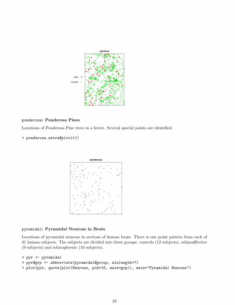
paracou

●

●

●

●

● ●

●

●

●

●

●

●●

●

●

●

●

●

●

●

●

●

●

●

●

●

●

● ●

●

●

●

●

●

●

●

●●

●

●● ●

●

●

●

●

●

juvenile

adult

ponderosa: Ponderosa Pines

Locations of Ponderosa Pine trees in a forest. Several special points are identified.

> ponderosa.extra$plotit()

ponderosa

●

●

●●

●

●

●

●

●●

●

●

●

●●

●●

●

● ●●

●

● ● ●

●

●

●

●● ●

●

●

●

●

● ●

●

●●

●●

●

●

●●

●

● ●

●● ●

●

●

●● ●

●

●

●●

●

●

●

●

●

●

● ●

●

● ●

● ●●

●

●

●

●

●

●

●

●●

●●

● ●

● ●●

●

●

●

●

●

●

●

●

●

●

●

●

●

●

●

●

●

A

B

C

pyramidal: Pyramidal Neurons in Brain

Locations of pyramidal neurons in sections of human brain. There is one point pattern from each of31 human subjects. The subjects are divided into three groups: controls (12 subjects), schizoaffective(9 subjects) and schizophrenic (10 subjects).

> pyr <- pyramidal

> pyr$grp <- abbreviate(pyramidal$group, minlength=7)

> plot(pyr, quote(plot(Neurons, pch=16, main=grp)), main="Pyramidal Neurons")

23

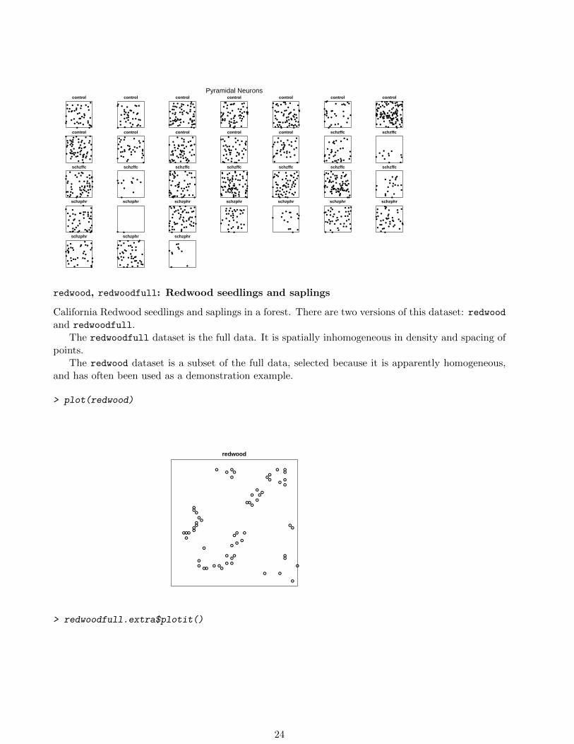
Pyramidal Neurons control

● ● ● ● ●●

●●●

●●

●●

● ●●

●●● ●

●●

●●●●●

●●● ●

●●●

●

●●

●●●●

●

●

control

●● ● ●● ●

●●

●

●●● ● ● ●●

●●●●

● ●●● ● ●●

●●

●●

●

●

●●●

●

● ●

control● ● ●● ●

●●

●

●●●●●●●

●● ● ●●●●●

● ●● ● ●

●●● ●

●●●●

● ●●●●●●● ●●

●● ●● ●●

●●●●●●● ●● ●●●

●●

control●●

● ●●●● ●●

● ●●●●

●

● ● ● ●● ●

●● ●●●

●

●●●●●●●●

●●

●●●●

● ● ● ● ●●

●●●

●●●● ●

●●

●●● ●

control●

●●●

●●●

● ●●

●●●

●●

●●● ●

●●

●●●●●

●●●●●●

●

●●

● ●● ●

●●

●●

●●●●●

●●●●●●●●

●●●

●●● ●

●●

control●●

●●

●●●●

●●● ●● ●

●●●

●● ●

●

●●●

●

●●

●●

● ●●

control● ● ● ●●● ●● ●

●●●●

●●●

●●

●●●●

●●● ● ●

●

●●●●

●● ●

● ●●●●

●●●

●●●●●

●●●●

●●●●

●●●● ●● ●● ●●●●● ●

●●●●●

●●●●●●●●●

● ●●●

●● ●

●●●●●●●

● ●

●● ●●

●●

control●

● ● ●●

●●●●

●●●●● ●●

●● ●

●

● ●● ●

●

●

●●●

●●●●●

●●

●●●●● ● ●

●●

●●●●●

●●●

●●

●● ●

●●

●

●●

control●

●●

● ●● ●●

●

●●● ● ●

●

●●●

●●

●●●

●●

●

●

●

● ●●

●●

●●

●

●●

control●

● ●

●●●●

●

● ● ●● ●●

● ●● ●

●

●

●

●●●●●

●●

●●●

●● ●

●●● ●

● ●

●●

●

●●●

●●●●

●●●

●●

●●

●

control

●●●

●

●●●

● ●

●●

●●●

●●

●●●

●●

●●●

●●

●●●●●●● ●

●●

●●●

●●

●●

●●●

control● ●

●●●●

●●●

●●

●●● ●

●●

●●

●●●●

●●●

● ● ●

●●

●●

● ●

●●

●

schzffc●

●●●●● ●●

●●● ●●● ●

● ●

●●

● ●● ●

●

● ●●●

●●●●

●●

● ●

schzffc

●● ●

●●

●●●

●

●

● ●

schzffc●

●● ●●

●●●●

●●

●●

●●● ●

● ● ● ●●●

●●●●

●●●

●●

●●

● ●● ●●●

● ●

●

●●

●●●

●●

●●

●●●

schzffc

● ●●

●

●●●● ●

●

●

●

schzffc●●● ●

●●

●●

●

●

●●●

●●

●

●●●●

●●

● ● ●●

● ● ●●●

●●●

●●●

●●●

●●●●●● ●

●

●●● ● ●

●

schzffc●● ●

●●●

●

●●●

●●●●●●

● ●

●●●

●● ● ● ●

●●

●

●●●

●●

●● ●●●● ●● ●

●

●●●●●●●

●●●●●

●●

●● ●●

●● ●●

● ●●

●●●●●

●●●●●

schzffc● ● ●

●

●●●●●●

●

●●

● ●● ●

● ●●

●●●●

●● ●●●●● ● ●

●●●●●●

●●

●● ● ● ●●

●●

●●

●●

●●●● ●

● ● ●

schzffc● ●

●●●●●●

●●●●

●●

●● ●

●●●●●

● ●●●●● ● ●

●●●●●

●

●●●●●●

●

●

●●●● ●● ●

●●●

● ●●●●●●●●●●

●●●●

●●●

●●●

●

schzffc

● ●●●●●

●

● ●●●●

●●

●●

●

●●●

●

schzphr●

● ●●

● ● ●●●

●● ● ●●●

●

● ●●●

●● ●

●●

●●●

● ● ●●

●●●●

●●●

●

●

●●●

●●●

schzphr

● ●

schzphr●

●●●

● ●● ●

●●●●

●●●

●●●

●

●●

●●●●

●●●●●

●

●●●●●

●●

●

● ●

●●●●

●

●● ●

●●

● ● ● ●●

●

schzphr

● ●●●●●●

●●●

● ● ●●

● ●

●●●●●

● ● ●●

● ●●

●●●

●●●

● ●

●

schzphr

●●

●●●

●

●●●●

●●

●● ●

●

schzphr●

●● ● ●

●●●●●●

●●

● ● ●●

●● ● ●

●

●●

●

●●●●

●● ●● ● ● ●

●●●

●●

● ●●

schzphr

●

●●●

● ● ●

●●●

●

●●●●● ●

●●

●●

●

●

●●●●

●●●

●

●● ●

●●●●

●●

●

schzphr

●●

●●

●●●●

●●●●

●●●

●●

●●

●●

●

●

●

●●●

● ● ● ●

●●

●

●● ●

●

schzphr● ● ●

●●●

● ● ●●●●

●●● ● ●

●●● ● ●

●●●●

●●●●●

●● ●● ●

●

●●●

●●

●

●●●

●

schzphr

●●

●●

●●●

●

●●

redwood, redwoodfull: Redwood seedlings and saplings

California Redwood seedlings and saplings in a forest. There are two versions of this dataset: redwoodand redwoodfull.

The redwoodfull dataset is the full data. It is spatially inhomogeneous in density and spacing ofpoints.

The redwood dataset is a subset of the full data, selected because it is apparently homogeneous,and has often been used as a demonstration example.

> plot(redwood)

redwood

●●

●

●

●

●●

●

●

●

●●

●

●

●●

●

●●●

●

●

●

●●

●●

●

●●●

●●

●●

●●

●

●●

●

●

●

●●

● ●●

●●

●

●● ●

● ●● ●●

● ●

●

> redwoodfull.extra$plotit()

24

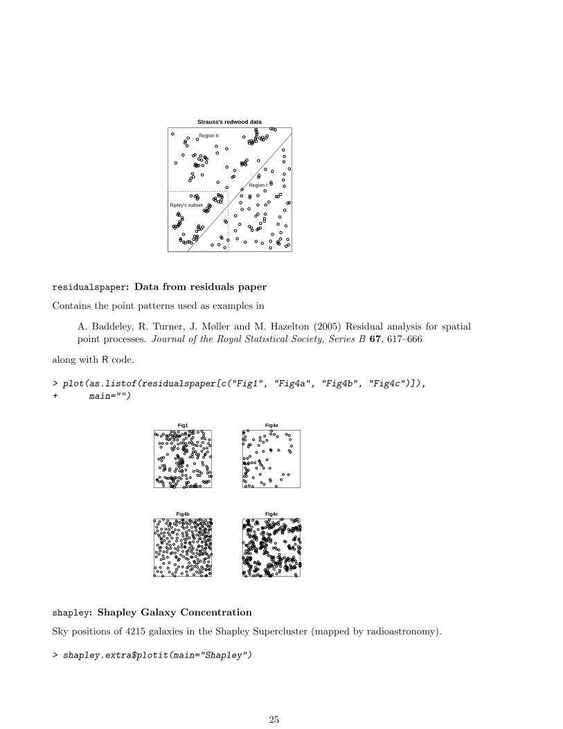
Strauss's redwood data

●

●

●

●●●

●●●

●●

●

●● ●

●●● ● ●●●

●● ●●● ●

●● ●

● ●● ● ●

●●●● ● ●●

●●● ●●●●●

●●

●● ● ● ●● ●● ●● ●● ●● ●● ●● ●

●●● ●●●● ●

●● ● ●● ●● ● ●● ●●● ●● ●●● ●●● ●

●

●●● ● ● ●●●● ●● ●●●● ● ●●● ●● ●●● ●● ●

●● ●

●● ●●●

●

●

●●● ●●● ●● ●● ● ●● ●●●●●●●●●●

●●●●●

●●●● ●●● ● ●●● ●●

●●

●●●● ●●●●●●● ●

Region I

Region II

Ripley's subset

residualspaper: Data from residuals paper

Contains the point patterns used as examples in

A. Baddeley, R. Turner, J. Møller and M. Hazelton (2005) Residual analysis for spatialpoint processes. Journal of the Royal Statistical Society, Series B 67, 617–666

along with R code.

> plot(as.listof(residualspaper[c("Fig1", "Fig4a", "Fig4b", "Fig4c")]),

+ main="")

Fig1

●●● ●

●●●

●●

●●●●●●

●● ●●

●

●●

●●● ●

● ●●●●● ● ●

● ●●● ●● ●

●●

●●●●

●

●

●

● ●● ●

● ●●●● ●●●●● ●

●●●●● ● ●●●●

●● ●●●

●● ● ●●● ●●●●●●●●●●●

●●●●

●●

●●●●●●● ●●●●

●●●●

●●●

●●●● ● ●● ● ●●

●●●

●●●

●● ●●●● ●●

●● ●●

●●● ●

●

●● ●

●●●

●●● ●●● ●

●●● ● ●

●●

●● ●●●

●●●

● ●●●

●●● ●

●●●●

●●●●

●

●

●

●

●

●

Fig4a

●

●

●

●●

●

●

● ●

●

● ●

●

●

●●

●

●

●●

●

●

●

●

●

●

●

● ●●

●

●

●

●● ●

●

●

●

●●

●

●

●

●

●

●

●

●●

●

●

●

●

●

●

●

●

●

●

●●

●

●

●

●

●●

●

●●

●

●

Fig4b

●

●

●

●

●

●

●

●

●●

●

●

●

●

●●

●

●

●

●

●

●

●

●

●●

●

●

●

●

●

●

●

●

●

●

●

●

●

●

●

●

●

●

●

●

● ●

●

●

●

●

●

●

●

●

●

●

●

●●

●

●

●

●●

●

●

●

●

●

●

●●

●

●●

●

●

●

●●

●

●

●

●

●

●

●

●

●

●

●

●

●

●

●

●

●

●

●

●

●

●

●

●

●

●

●●

●

●

●

●

●

●

●

●

●

●

●

●

●

●

●

●

●

●

●●

●

●

●

●

●

●

●

●● ●

●●

●

●

●

●

●

●

●

●●

●

●

●

●

●

●

●●

●

●

●

●

●●

●

●

●

●

●

●

●

●

●●

●

●

●

●●

●

●

●

●

●

●

●

●

●

●

●●

●

●

●

●

●

●

●●

●

●●

●

●

●

●

●

●

●

●

●

●

●

●

●

●●

●

●

●

●

●

●

●

●

●

●

●● ●

●

●

●

●

●

●

●

●●

●

●

●

●

●

●

● ●

●

●

●

●

● ●

●

●

●

●

●

●

●

●

●

●

●

●

●

●

●

●

●

Fig4c

●

●

●

●

●

●●

●

●

●

●

●

●

●

●

●

●

●

●

●

●

●

●

●

●

●

●

●

●

●

●

●

●●

●

●

●

●

●

●

●

●

●

●

●

●

● ●

●

●

●

●

●●

●

●

●

●

●

●

●

●●

●

●

●

●

●

●

●

●

●

●

●

●

●

●

●

●

●

●●

●

●

●

●

●

●

●●

●

●

●

●●

●

●

●

●

●●

●

●

●

●

●

●

●

●

●

●

●

●

●

●

●

●

●

●

●

●

●

●

●

●

●

●

●

●

●

●

●

●

●

●

●

●

●

● ●

●

●

●

●

●

●

●

●

●●

●

●

●●

●

●

● ●

●

●

●

●

●

●

●

●

●●

●

● ●

●

●

●

●

●

●

●● ●

●●

●●

●

●

●

●

●

●

●

●

●

●

●

●

●

●●

●

●

●

●●

●

●

●

●

●

●

●

●

●

●

●

●

●

●●

●

●

●

● ●

●

●

●

●

●

●

●

●

●

●

●

●

●

●

●●

●

●

●

●

●

●

●

●

●

●●

●

●

●

●●

●

●

●

●

●

●

●

● ●●

●

●

●

●

●

●

●

●●

●

●

●

●●●

●●

●

●

●

●

●

●

●

●

●

●

●

●

●

●

●

●●

●

●

●

●

●

●●

●●

●

●

●

●

●●

●

●

●

●

●

●

●

●

●

●

●

●

●

●

●

●

●

●

●

●

●

●

●

●

●

●

●

●

●

●

●

●

●

●

●

●

●

● ●

●

●

●

●

●

●

●

●

●

●●

●

●

●

●

●

●

●

● ●

●

●

shapley: Shapley Galaxy Concentration

Sky positions of 4215 galaxies in the Shapley Supercluster (mapped by radioastronomy).

> shapley.extra$plotit(main="Shapley")

25

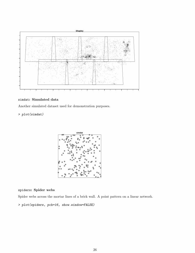
Shapley

−38

−36

−34

−32

−30

−28

simdat: Simulated data

Another simulated dataset used for demonstration purposes.

> plot(simdat)

simdat

●

●

●

●

●

●

●

●●

●

●

●

●

●

● ●

●

●

●

●

●

●●

●

●

●

●

●

●

●

●

●

●

●

●

●

●

●

●

●

●

●

●

●

●

●

●

●

●

●

●

●

●

●

●

●

●

●

●

●

●

●

●

●

●

●

●

●●

●●

●

●

●

●

●

●

●

●

●

●

●

●

●

●

●

●

●

●

●

●

●

●

●

●

●

●

●

●

●

●

●

●

●

●

●

●

●

●

●

●

● ●●

●●

●

●

●

●

●

● ●

●

●

●

●

●

●

●

●

●

●

●

●

●

●

●

●

●

●

●

●

●

●

●

●

●

●

●

●

●

●

●

●

●

●

●

●

●

●

●

●

●

●

●

●

●

●

●

●

●

●

●●

●

● ●

●

●

●

●

●

●

●

●

●

●

●

●

●

●

●

●

●

●

●

spiders: Spider webs

Spider webs across the mortar lines of a brick wall. A point pattern on a linear network.

> plot(spiders, pch=16, show.window=FALSE)

26

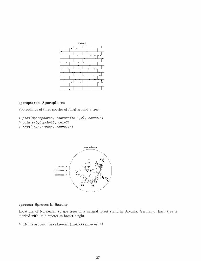
spiders

●

● ● ●● ●

● ●● ● ● ● ● ●

● ● ● ●

● ● ● ● ●

● ● ● ● ● ●

● ●

● ● ● ●

●● ●

● ● ●● ● ●

● ●

● ●

sporophores: Sporophores

Sporophores of three species of fungi around a tree.

> plot(sporophores, chars=c(16,1,2), cex=0.6)

> points(0,0,pch=16, cex=2)

> text(15,8,"Tree", cex=0.75)

sporophores

●●●

●●●●

●●

●●●

●●● ●●●

●●●●●●●

●

●●

●●●●●●

●●

●● ●●●●●●

●● ●●●●●●

●

●

●●●●

●●●●●

●

●●

●●●●

●●

●●●●

● ●●

● ●●●●●●

●●●●●●●●

●

●●●●●

●●●●●●

●●●

●●●

●●●●●●●●●

●

●●●●

●●

●● ● ●●●●

●●●

●●

●●●●

●●●●

●●●●●

●●●●

●●●●●●●●● ●

●●

●●

●●

●●●●●●

●●●●

●●●

●●

●

●

●● ●

●●●

●

●●

●

●

●

●

Hebloma spp

L pubescens

L laccata

●Tree

spruces: Spruces in Saxony

Locations of Norwegian spruce trees in a natural forest stand in Saxonia, Germany. Each tree ismarked with its diameter at breast height.

> plot(spruces, maxsize=min(nndist(spruces)))

27

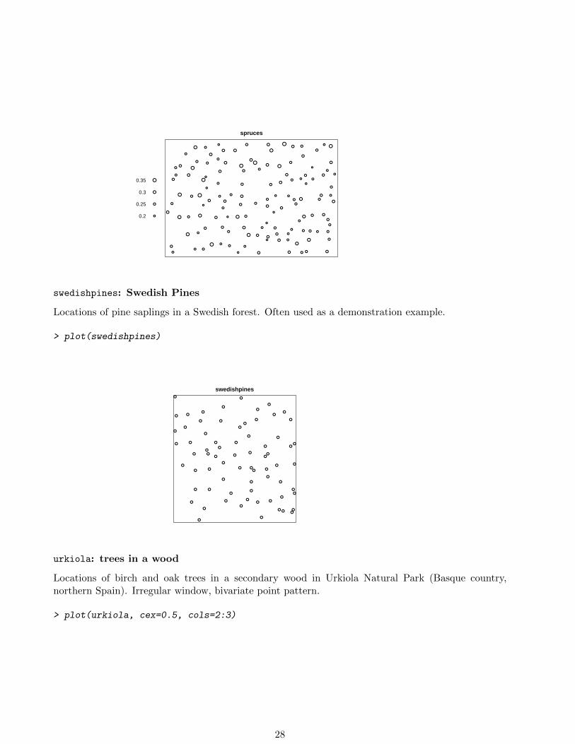
spruces

●

●

●

●

●

●

●●

●

●

●

●

●

●

●

● ●

● ●

●

●

● ●

●

●

●

●

●

●

●

●

●

●

●

●

●

●

●

●

●

●

●

●

●

●

●●

●

●

●

●

●

●●

●

●

●

●

●

●

●

●

●

●

●●

●

●

●

●

●

●

●

●

●

●

● ●

●

●●

●

●

●

●

●

●

●

●

●

●

●

●

●

●

●

●

●

●

●

●

●

●

●

●

●

●

●

●

●

●

●

●

●

●

●

●

●

●

●

●

●●

●

●

●

●

●

●

●

●

●

●

●

●

●

●

●

0.2

0.25

0.3

0.35

swedishpines: Swedish Pines

Locations of pine saplings in a Swedish forest. Often used as a demonstration example.

> plot(swedishpines)

swedishpines●

●

●

●

●

●

●

●

●

●

●

●

●

●

●

●

●

●

●

●

●

●

●

●

●

●

●

●

●

●

●

●

●

●

●

●

●

●

●

●

●

●

●

●

●

●

●

●

●

●

●

●

●

●

●

●

●

●

●

●

●

●

●

●

●

●●

●

●

●

●

urkiola: trees in a wood

Locations of birch and oak trees in a secondary wood in Urkiola Natural Park (Basque country,northern Spain). Irregular window, bivariate point pattern.

> plot(urkiola, cex=0.5, cols=2:3)

28

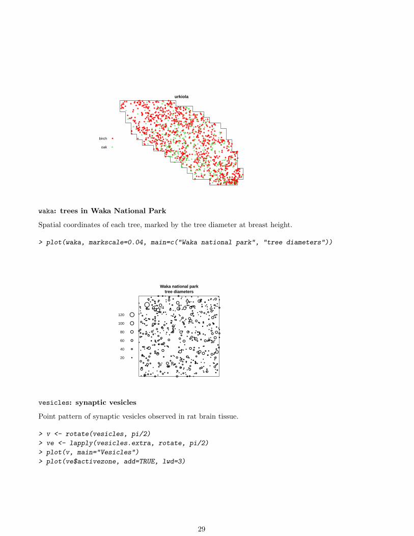
urkiola●●

●

●●

●●

●●●

●

●

●

● ●

●●

●

●

●

● ●

●●

●●

●

●●

●

●●

● ●

●●

●

●●●

●●

●

●●

●

●

●

●●●

●

●●

●

●

●●

●

●

●●

●●

●

●

● ● ●

● ●

●

●

●

●

●●●

●●●

●●●

●

●●●

●●

●

●

●

●●

●

●●

●

●●

●

●

●●

●

●●●●●●

●●●

●

●

●●●●

●●

●

●

●

●

●●

●

●●

●●

●

●●

●●

●●● ●

●

●●

●

●

●

●

●●

●●●

●

● ●●●

●

●

●

●

●●●●

●

●●

●

● ●●●●

●●●

●

●

●●

●●●

●●

●

●●●

●

●●

●

●●

●●●

●

●●●

●●●

●●

●

●●●

●

●●

●

●●

●●

●

●

●

●●●

●●

● ●●

●●●

●●

●

●●

●

●

●

●●●●

●

●●●

●●

●

●

●●●●

●

● ●●

●●●

●●

●

●●

● ●●

●

●

●

●●●

●●●

●●●

●

●●

●

●

●

●

●

●

●●●

●●

● ●●

●●

●●

●

●

●●●

●●●

●●

●

●

●

●●●●

●●

●●

●

●

●

●

●●

●●

●

●

●

●●●

●

●●

●●●

●●

●●●●

●●

●

●

●

● ●●

●●

●●

● ●●

●

●●

●

●

●

● ●

●

●●●

●

●

●

●

●

●●●●●

●

●

●

●●

●●

●

●

●

●●

●

● ● ●●

●●

●

●

●●

●

●●

●

●

●●●

●

●

●

●●●

●

●

●●●●●●●●

●

●

●●

●

●

●●●

●

●

●●

●

●●

●

●

●

●●●

●

●

●

●

●

●

●

●

●●

●●

●

●●

● ●●●●

●

●●

●

●

●

●●

●●

●●

●

●

●

●●

●●

●

●●

●

●●●●

●

● ●

●

●

●

●

●

●

● ● ● ●

●●●●●

●

●

●

●

●

●

●

●

●●

●●

●●

●●

●

●●

●●

●

●

●●●

●●

●

●

●

●

● ●●●

● ●●

●

●

●

●●

●

●●●

●

●

●●

●

●●

●

●

●●

●

●●

●●

● ●

●

●

●●

●

●●

●

●

● ●

●●

●●

●●

●

●

●

●

●●

●●

●

●

●●

● ●

● ●

●

●

●●●

●

● ● ●●

●

●●

●

●●

●

●

●

●

●

●

●

●

●●

●●

●

●

●●

●●

●●

● ●●●

●

●●

●

●●

●●●●●

●●

●

●●

●●

●

●

●

●●

●●

●

●● ●

● ●●

●●

●

●●

●

●

●

●

●

●●

●

●●●

●

●

●

●

● ●●●●

●●

●

●

●

●

●

●●●

●●●

●

●●

●●

●●●

●●

●●●●

●

●●

● ●

●

●●

●●●

●

●

●●●

●

● ●

●●

●

●●

●

●●●

●●●

●●

●●●●●

●●●

●

●

●

●●●●

● ●

● ● ●●

●● ●

●●●●

●● ●●

● ●●

●●●●

●

●

●●

●●

●

●

●

●●●

●●●●

●

●●●

●●

●●●

●●●

●●●●●

●●

●

●●●

●●

●●●●

●

●

●

●

●

●●

● ●

●

●●●

●●●● ●

●

●

oak

birch

waka: trees in Waka National Park

Spatial coordinates of each tree, marked by the tree diameter at breast height.

> plot(waka, markscale=0.04, main=c("Waka national park", "tree diameters"))

Waka national parktree diameters

●●●●

●

●●

●● ●

●●

●

●

●●

●●

●

●

●

●●● ●

●

●

●●●

●●●

● ●

●●

●

●

●

● ●

●●

●

●●

●

●

●

●●

●

●●

●●

●●

●

●●

●

●

●

●

●

●

●●

●

●●●

●●

●●

●● ●

●●

●

●

●

●

●

●

●

●●●

●

●●●

●

●●

●●●●

●●●●

●

●●●

●

●● ● ●

●

●

●●●●

●●

●

●●

●

●● ●●

●

● ●●

●

●

●● ●●

●

●

●

●

●

●●

●

● ●

●

●

●

●●

●

●

●

● ●

●

●

●

●●

●

●

●

●

●

●●

●

●

●

●●

●

●●

●●

●

●● ●

●●

●

●● ● ●

●

●●

●●

●

●

●●●●

● ●

●

●

●

●●

●●●

● ●

●

●

●●

●

●

●

●●

●

●●

●

●●

●●

●

●

●

●

●

●

●●●

●

●●

●

●

●●

●●

●●

●

●●

●

●

●

●●

●

●

●●●

●

●

●●●

●●● ●●

●●

●

●●

●●●

●

●●●

●

●

●●

●●

●

●

●

●

●●

●

●

●●

●

●●●●●

●

● ●●

●●

●●●

●

●

●●

●●

●

●

●

●

●●

●

●●

● ●

●●

●

●●

●

●

●●●

●●

●● ●

●

●● ●●● ●

●

●●

●●●

●●

●●●

●●

●

●

●

●

●

●●●

●●

●

●

●

●● ●

●

●●

●●

● ●

●●

●●●

●●

●

●

●●●

●

●

●

● ●●

●●

●

●

●

●

●

●

●●

● ●

● ●

●●

●

●

●●●

●

●●

●

●

● ●●●

●

●●

●

●

● ● ●

●

●●●

●

● ●●

●●

●

●

●

●

●

●

●●

●

●

●

●●

●●●

●

●

●

●

●

●

●

●●●

●

●

● ●

●

●●

●●

● ●

●

●●

●

●

●

●

●

●

●

20

40

60

80

100

120

vesicles: synaptic vesicles

Point pattern of synaptic vesicles observed in rat brain tissue.

> v <- rotate(vesicles, pi/2)

> ve <- lapply(vesicles.extra, rotate, pi/2)

> plot(v, main="Vesicles")

> plot(ve$activezone, add=TRUE, lwd=3)

29

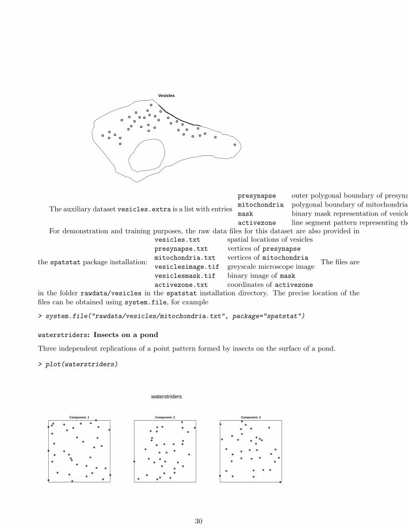
Vesicles

●

●

●

●● ●

●

●

●

●

●

●

●●

●

●●

●

●

●●

●●

●

●●

●

●

●

●

●

● ●●

●

●

●

The auxiliary dataset vesicles.extra is a list with entries

presynapse outer polygonal boundary of presynapsemitochondria polygonal boundary of mitochondriamask binary mask representation of vesicles windowactivezone line segment pattern representing the active zone.

For demonstration and training purposes, the raw data files for this dataset are also provided in

the spatstat package installation:

vesicles.txt spatial locations of vesiclespresynapse.txt vertices of presynapsemitochondria.txt vertices of mitochondriavesiclesimage.tif greyscale microscope imagevesiclesmask.tif binary image of maskactivezone.txt coordinates of activezone

The files are

in the folder rawdata/vesicles in the spatstat installation directory. The precise location of thefiles can be obtained using system.file, for example

> system.file("rawdata/vesicles/mitochondria.txt", package="spatstat")

waterstriders: Insects on a pond

Three independent replications of a point pattern formed by insects on the surface of a pond.

> plot(waterstriders)

waterstriders

Component_1

●

●

●●

●

●

●

●

●

●

●

●

●

●

●

●

●

●

●

●

●

●

●

●

●

●

●

●

●

●

●

●

●

●

●

●

●

●

Component_2

●

●

●

●

●

●

●

●

●

●

●

●

●

●

●

●

●

●

●

●

●

●

●

●

●

●

●

●

●

●

●

●

●

●

●

●

Component_3

●

●

●

●

●

●

●

●

●

●

●

●

●

●

●

●

●

●

●

●

●

●

●

●

●

●

●●

●

●

●

●

●

●

●

●

30